Sage Journals: Discover world-class research

Abstract

In recent years, the popularity of procedures for collecting intensive longitudinal data, such as the experience-sampling method, has increased greatly. The data collected using such designs allow researchers to study the dynamics of psychological functioning and how these dynamics differ across individuals. To this end, the data are often modeled with multilevel regression models. An important question that arises when researchers design intensive longitudinal studies is how to determine the number of participants needed to test specific hypotheses regarding the parameters of these models with sufficient power. Power calculations for intensive longitudinal studies are challenging because of the hierarchical data structure in which repeated observations are nested within the individuals and because of the serial dependence that is typically present in these data. We therefore present a user-friendly application and step-by-step tutorial for performing simulation-based power analyses for a set of models that are popular in intensive longitudinal research. Because many studies use the same sampling protocol (i.e., a fixed number of at least approximately equidistant observations) within individuals, we assume that this protocol is fixed and focus on the number of participants. All included models explicitly account for the temporal dependencies in the data by assuming serially correlated errors or including autoregressive effects.

Keywords

power analysis Monte Carlo simulation intensive longitudinal designs linear mixed-effects models multilevel autoregressive models open materials

Over recent years, psychological research has increasingly focused on investigating how complex psychological processes evolve dynamically across time within single individuals. To this end, researchers use intensive longitudinal (IL) designs and data-collection methods, such as the experience-sampling method (ESM; Myin-Germeys et al., 2009, 2018), in which individuals are repeatedly measured. The repeated measurements allow researchers to study dynamic aspects of psychological functioning within individuals and individual differences in these dynamics. Examples of such dynamics are emotional variability and stability and emotional inertia (Kuppens & Verduyn, 2015). Individual differences in these dynamics have been consistently linked to individual differences in well-being and health (e.g., Brose et al., 2015; Dejonckheere et al., 2018; Kuppens et al., 2010).

Given the increased focus on dynamic psychological processes within individuals, it is no surprise that the recent debate on the reproducibility and transparency of psychological research (Munafò et al., 2017) has led to the development of guidelines for conducting IL research (Trull & Ebner-Priemer, 2020) and the promotion of open-science practices in IL research (Kirtley et al., in press). Here, we aim to continue along this path and focus on sample-size planning for IL designs. A fixed sampling schedule within individuals is common practice in IL studies not only for the reasons outlined in the previous paragraph, but also because of its feasibility and because it reduces the participants’ burden. Therefore, we focus on assessing the number of participants needed while assuming a fixed number of (at least approximately) equidistant observations within individuals. Adequate sample-size planning allows control of the accuracy and power of statistical testing and modeling and is therefore of crucial importance for the replicability of empirical findings (see Ioannidis, 2005; Szucs & Ioannidis, 2017).

Although power analyses are often used to inform sample-size planning in general (Cohen, 1988), they are not yet well established in IL research. One reason for this is that performing power calculations to select the number of participants in the context of IL studies is challenging because of the intricacies of the data (Bolger, 2011; De Jong et al., 2010). First, IL data have a multilevel structure, in that repeated observations are nested within individuals. Second, observations are closer in time in comparison with traditional longitudinal designs. This likely leads to considerable temporal dependencies between data measured at adjacent observations. As we noted earlier, it is often the very purpose of an IL study to capture such temporal dependencies, as they reflect psychological dynamics that are often of inherent interest.

But not only the data structure is complicated; the applied statistical models are as well, as they should capture such dynamics and individual differences therein. First, the models have to distinguish interindividual differences from intra-individual changes (e.g., Hamaker et al., 2015; Molenaar, 2004). Multilevel regression approaches offer an established way of doing this. Second, models should also take temporal dependencies into account, either to control for them or to quantify and model them. This requires that one includes either serially correlated errors or the lagged outcome variable as a predictor in the multilevel models. Although there are several resources available to help researchers perform power analyses for multilevel models (e.g., Arend & Schäfer, 2019; Browne et al., 2009; Cools et al., 2008; Green & MacLeod, 2016; Hedeker et al., 1999; Landau & Stahl, 2013; Lane & Hennes, 2018; Mathieu et al., 2012; Raudenbush, 1997; Raudenbush & Liu, 2001; Snijders & Bosker, 1993; Zhang, 2014; Zhang & Wang, 2009), these do not account for the temporal dependencies that characterize IL data.

We therefore present a user-friendly application for performing simulation-based power analyses for IL studies. The obtained power results can inform sample-size planning by shedding light on the number of participants needed to obtain accurate and significant parameter estimates. The application was developed in R (R Core Team, 2020) using the shiny package (Chang et al., 2019). It covers a set of models that are widely used to study individual differences in IL studies and properly account for the temporal dependency.

In this article, we first briefly review existing approaches to computing power in multilevel models and then discuss the multilevel models that are covered by our application. Next, we introduce the Shiny app and discuss how it can be used for sample-size planning. Using an already published data set, we illustrate how to perform sample-size planning with the app. We conclude the article with a general discussion of additional considerations and possible extensions.

Disclosures

The R code for the Shiny application is available via a Git repository hosted on GitHub at https://github.com/ginettelafit/PowerAnalysisIL and via OSF at https://osf.io/vguey/. The OSF project also includes the R Markdown document used in the illustrations.

Power Analyses in Intensive Longitudinal Studies

We use statistical power as the criterion for estimating the number of participants needed in an IL study. High power is desirable because it improves the reproducibility of research findings and prevents the overestimation of effect sizes (see Ioannidis, 2005; Szucs & Ioannidis, 2017). Formally, power is defined as the probability of correctly rejecting the null hypothesis when the alternative hypothesis is true in the population under study (Cohen, 1988). The power to detect an effect is therefore determined by the size of the effect in the population, the predetermined Type I error rate (i.e., the significance level), and the standard error of the test statistic used. Power is higher if the population effect is larger, the Type I error rate is higher, and the standard error of the test statistic is smaller. The standard error, in turn, is related to sample size, in that larger sample sizes lead to smaller standard errors. The latter point explains why power analysis can inform sample-size planning.

In general, two approaches can be used for performing power analysis: the analytic approach and the simulation-based approach. In the analytic approach, power is determined by using formulas for the standard errors of the estimated effects, expressing them as a function of the parameters of the multilevel model under study and the sample size. Using these formulas, it is possible to estimate the sample size that allows reaching a predetermined value of power (see, e.g., Cohen, 1988; Hedeker et al., 1999; Moerbeek & Maas, 2005; Moerbeek et al., 2000, 2001; Raudenbush, 1997; Raudenbush & Liu, 2001; Snijders & Bosker, 1993; C. Wang et al., 2015). However, as is true for many other complex models, so far no analytic formulas have been derived for multilevel models that include temporal dependencies (see Arend & Schäfer, 2019). Also, the analytic approach usually relies on asymptotic estimation theory and might, therefore, be inaccurate in practice when dealing with small numbers of participants and measurements per participant. For example, Snijders and Bosker (1993) determined the optimal sample sizes for two-level linear models by using normal approximations for the distribution of the estimated coefficients. However, in small samples, the distribution of the estimator can be nonnormal and is potentially heavy-tailed, which results in unreliable standard error estimates.

The simulation-based approach uses the hypothesized population model and concrete specifications of the associated parameters to generate a large number of data sets. Each of these data sets is then analyzed with the model under study and the parameters of interest are tested for significance. Because the data have been randomly generated, the parameter estimates and the test results will vary across the data sets. Hence, one can compute the power as the proportion of simulated data sets for which the null hypothesis about the parameters of interest has been rejected (see, e.g., Arend & Schäfer, 2019; Astivia et al., 2019; Bolger, 2011; Browne et al., 2009; Cools et al., 2008; Green & MacLeod, 2016; Landau & Stahl, 2013; Lane & Hennes, 2018; Maas & Hox, 2005; Mathieu et al., 2012; Zhang, 2014; Zhang & Wang, 2009). Performing these calculations while varying the number of participants allows one to determine the number of participants necessary to reach a predetermined level of power (e.g., 80%). The simulation-based approach is a good alternative when analytic formulations are not available or too difficult to derive. Therefore, we adopt this approach in this article, given the complexity of IL data and associated modeling questions.

Population Models of Interest

We focus on a set of research questions regarding IL data that can be addressed using specific multilevel regression models (Raudenbush & Bryk, 2002). Figure 1 provides a graphical representation of the different models. These models correspond to a hypothetical data set that we use for illustration purposes and are covered by the application we introduce in the next main section. Table 1 shows a few rows of this data set involving individuals diagnosed with major depressive disorder (MDD) and healthy control individuals. The participants responded to momentary questionnaires at six equidistant time points. The first column contains the participants’ identification numbers, and the second column the observation numbers. The third and fourth columns contain the data for the Level 1, or time-varying, variables: affect (for negative affect) and anhedonia, which were measured at every observation. The final two columns contain the data for two Level 2, or time-invariant, variables. The depression variable refers to the sum score on a continuous self-report instrument assessing the experience of depressive symptoms at baseline. Finally, diagnosis is a binary variable that equals 1 for participants diagnosed with MDD and 0 otherwise. Formulas for the models in Figure 1 are given in Table 2, and Table 3 provides an overview of the effects of interest.

Fig. 1.

Graphical representation of the population models of interest.

Table 1.

Example Rows of the Hypothetical Data Set

PID	Observation	Affect	Anhedonia	Depression	Diagnosis
1	1	28.8	42	12	1
1	2	26.0	30	12	1
1	3	27.4	22	12	1
1	4	21.4	33	12	1
1	5	14.4	23	12	1
1	6	26.6	18	12	1
2	1	16.0	19	4	0
2	2	13.2	23	4	0
2	3	9.6	12	4	0
2	4	14.4	18	4	0
2	5	8.6	10	4	0
2	6	9.2	15	4	0

Note: Affect (negative affect) and anhedonia are the Level 1 variables, and depression and diagnosis are the Level 2 variables. PID = participant identification number.

Table 2.

Formulas for the Models in Figure 1 and Available in the PowerAnalysisIL Application

		Level 2
Model	Level 1	Random intercept	Random slope
Model 1	affect_it = γ_0i + ε_it	γ_0i = β₀₀ + β₀₁diagnosis_i + v_0i	—
Model 2	affect_it = γ_0i + ε_it	γ_0i = β₀₀ + β₀₁depression_i + v_0i	—
Model 3	affect_it = γ_0i + γ_1i anhedonia_it + ε_it	γ_0i = β₀₀ + v_0i	γ_1i = β₁₀ + v_1i
Model 4	affect_it = γ_0i + γ_1i anhedonia_it + ε_it	γ_0i = β₀₀ + v_0i	—
Model 5	affect_it = γ_0i + γ_1i anhedonia_it + ε_it	γ_0i = β₀₀ + β₀₁diagnosis_i + v_0i	γ_1i = β₁₀ + β₁₁diagnosis_i + v_1i
Model 6	affect_it = γ_0i + γ_1i anhedonia_it + ε_it	γ_0i = β₀₀ + β₀₁diagnosis_i + v_0i	—
Model 7	affect_it = γ_0i + γ_1i anhedonia_it + ε_it	γ_0i = β₀₀ + β₀₁depression_i + v_0i	γ_1i = β₁₀ + β₁₁depression_i + v_1i
Model 8	affect_it = γ_0i + γ_1i anhedonia_it + ε_it	γ_0i = β₀₀ + β₀₁depression_i + v_0i	—
Model 9	affect_it = γ_0i + γ_1i affect_it−1 + ε_it	γ_0i = β₀₀ + v_0i	γ_1i = β₁₀ + v_1i
Model 10	affect_it = γ_0i + γ_1i affect_it−1 + ε_it	γ_0i = β₀₀ + β₀₁diagnosis_i + v_0i	γ_1i = β₁₀ + β₁₁diagnosis_i + v_1i
Model 11	affect_it = γ_0i + γ_1i affect_it−1 + ε_it	γ_0i = β₀₀ + β₀₁depression_i + v_0i	γ_1i = β₁₀ + β₁₁depression_i + v_1i

Table 3.

Overview of the Effects of Interest for the Models in Figure 1 and Available in the PowerAnalysisIL Application

Model	Time-varying Level 1 predictor		Time-invariant Level 2 predictor		Random intercept	Random slope	Cross-level interaction effect
Model	Continuous variable	Lagged dependent variable	Dummy variable	Continuous variable	Random intercept	Random slope	Cross-level interaction effect
Model 1	—	—	X	—	X	—	X
Model 2	—	—	—	X	X	—	X
Model 3	X	—	—	—	X	X	—
Model 4	X	—	—	—	X	—	—
Model 5	X	—	X	—	X	X	X
Model 6	X	—	X	—	X	—	X
Model 7	X	—	—	X	X	X	X
Model 8	X	—	—	X	X	—	X
Model 9	—	X	—	—	X	X	—
Model 10	—	X	X	—	X	X	X
Model 11	—	X	—	X	X	X	X

Group differences in mean level

Model 1 in Figure 1 estimates differences between the two groups of individuals in the mean of the outcome variable affect (e.g., Heininga et al., 2019; Myin-Germeys et al., 2001, 2003). This model includes the affect_it value as the outcome variable for the ith individual at the tth observation and a Level 2 dummy variable that indicates the diagnosis group (i.e., diagnosis_i). For participants in the reference group (healthy control participants), the mean level of affect equals β₀₀; for individuals diagnosed with MDD, the mean level of affect is given by β₀₀ + β₀₁. Within both diagnosis groups, interindividual differences in affect are modeled by the random intercept γ_0i. The random intercept expresses the deviation of each participant’s affect level from the group-specific mean level. It is normally distributed, and the standard deviation is denoted by $σ_{v_{0}}$ . To account for the likely temporal dependencies in IL data, we allow for serially correlated errors. Therefore, we assume that the Level 1 errors ε_it follow a first-order autoregressive (AR(1)) process (Goldstein et al., 1994); the correlation between two consecutive errors is denoted by ρ_ε, and σ_ε is the standard deviation of the Level 1 errors.¹ To guarantee that the model is stationary (Hamilton, 1994), the autocorrelation ρ_ε should range between −1 and 1. In Model 1, the main effect of interest is β₀₁ (i.e., the size of the average group difference), and we test whether it is statistically different from zero. As for all tests that we discuss, the hypothesis test is two-sided, and significance is evaluated with a Wald-type test statistic using a t distribution (Snijders & Bosker, 2011).

Effect of a Level 2 continuous predictor on the mean level

Model 2 in Figure 1 focuses on the effect of a continuous Level 2 predictor on the outcome of interest.² For the hypothetical data set, we investigate whether the individual-specific depression level, depression_i, predicts individual differences in the mean level of affect_it as captured by the random intercept γ_0i. These random intercepts are assumed to be normally distributed with mean β₀₀ + β₀₁depression_i and standard deviation $σ_{v_{0}}$ . We again assume an AR(1) structure for the Level 1 errors ε_it. When testing the effect of interest, β₀₁, we can grand-mean-center the Level 2 predictor to obtain a meaningful zero point for this predictor to render the intercept interpretable (Enders & Tofighi, 2007; Raudenbush & Bryk, 2002).

Effect of a Level 1 continuous predictor

Next, we focus on the effect of a continuous Level 1 predictor on the outcome, through Models 3 and 4 in Figure 1. For example, we might be interested in the extent to which anhedonia_it predicts affect_it in individuals diagnosed with MDD. Model 3 specifies a corresponding multilevel model with AR(1) Level 1 errors. The mean slope of anhedonia_it is denoted by β₁₀, which is the parameter of interest. This model captures interindividual differences by including a random intercept γ_0i and a random slope γ_1i. These random effects are bivariate normally distributed. β₀₀ then indicates the mean of the random intercepts, and β₁₀ the mean of the random slopes. Their standard deviations are denoted by $σ_{v_{0}}$ and $σ_{v_{1}}$ , respectively. The correlation between the random effects is given by $ρ_{v_{01}}$ (and the covariance between the random effects is denoted by $σ_{v_{01}}$ ). Model 4, on the other hand, assumes that the slope of anhedonia_i does not vary across participants. In both models, person-mean centering the Level 1 predictor is recommended because the fixed slope β₁₀ then provides an estimate that reflects only the (average) within-person association between the predictor and outcome (Enders & Tofighi, 2007; Raudenbush & Bryk, 2002).

Group differences in the effect of a Level 1 continuous predictor

Models structured like Models 5 and 6 in Figure 1 correspond to a class of multilevel models that are used to investigate differences between two groups of participants with respect to the association between a Level 1 predictor and the outcome of interest (while assuming AR(1) errors). In our illustration, these models thus include the outcome affect_it, the Level 1 predictor anhedonia_it, the Level 2 variable diagnosis_i, and a cross-level interaction (Raudenbush & Bryk, 2002) between the Level 1 and Level 2 predictors. β₀₀ and β₀₀ + β₀₁ represent the mean intercept of all individuals in the reference (healthy) and MDD groups, respectively. The mean slope for the reference group is indicated by β₁₀, and the mean slope for the MDD group amounts to β₁₀ + β₁₁. Therefore, the effect of interest is the difference between the two groups in the mean slope, β₁₁. Model 5 includes random intercepts γ_0i as well as random slopes γ_1i. Model 6 is more restrictive and does not include random slopes.

Cross-level interaction between two continuous predictors

Models 7 and 8 in Figure 1 focus on a cross-level interaction between the continuous Level 2 predictor depression_i and the continuous Level 1 predictor anhedonia_it (e.g., Arend & Schäfer, 2019), to investigate whether the level of depression (as measured at baseline) moderates the effect of anhedonia on affect. Therefore, the effect of interest is again β₁₁. As was the case for Models 5 and 6, Model 7 includes both random intercepts and random slopes, whereas Model 8 assumes that the slope does not vary across participants.

Multilevel autoregressive models

Models 9 to 11 (see Fig. 1) are multilevel AR(1) autoregressive models (Hamaker & Grasman, 2015) that explicitly focus on the amount of temporal dependence in the outcome. In such models, the lagged outcome variable (i.e., the observed outcome at the previous measurement occasion) is included as the predictor of interest. Such autoregressive effects have been extensively studied, for example, in affective research (Kuppens et al., 2010). Model 9 allows us to study the mean autoregressive effect across individuals as well as individual differences therein, through β₁₀ and γ_1i, respectively. To satisfy the stationarity assumption of the model, both effects have to range between −1 and 1. Given that temporal dependence is now captured through the autoregressive effect, the residuals ε_it are assumed to be independent and normally distributed with mean 0 and standard deviation σ_ε. Some researchers person-mean-center the lagged outcome variable, although Hamaker and Grasman (2015) showed in an extensive simulation study that this results in an underestimation of β₁₀. The resulting bias will have an impact on power.

Model 10 extends Model 9 in that it allows us to estimate the difference in the mean autoregressive effect between two groups of individuals (L. P. Wang et al., 2012). The mean autoregressive effect is β₁₀ for the reference group (healthy control individuals) and β₁₀ + β₁₁ for the MDD group. Therefore, the effect of interest is β₁₁.

Finally, models structured like Model 11 are used to estimate a cross-level interaction effect between a continuous Level 2 predictor and the lagged outcome, to study if the Level 2 predictor moderates the autoregressive effect (e.g., Brose et al., 2015; Koval et al., 2013). Consequently, β₁₁ is the effect of interest. In this case, Hamaker and Grasman (2015) clearly recommended person-mean centering the lagged predictor.

A Shiny App to Perform Power Analysis

In this section, we present the Shiny app, PowerAnalysisIL, that we developed to compute power as a function of the number of participants for the models described in the previous section. Figure 2 shows a screenshot of the opening page of the app, where users select the population model of interest, set the parameter values, and run their power analysis. The app was implemented using the R package shiny. It is available via a Git repository hosted on GitHub at https://github.com/ginettelafit/PowerAnalysisIL. Users can download the app and run it locally on their computer in R or RStudio (RStudio Team, 2015). In what follows, we describe how the app works.

Fig. 2.

Screenshot of the opening page of PowerAnalysisIL, a Shiny app to perform power analysis to select the number of participants in intensive longitudinal studies.

App input

First, the user indicates which multilevel model (i.e., Model 1–Model 11) will be used to estimate the effect of interest and specifies plausible values for all model parameters. For instance, if one wants to focus on differences in mean affect between individuals diagnosed with MDD and healthy control individuals, one selects Model 1. Next, the sample sizes that should be considered in the power computations have to be provided. In the case of Model 1, one has to set a range of values for the number of participants in the reference (healthy) group and the number of participants diagnosed with MDD. Using this information, the software will create a Level 2 dummy predictor indicating group membership for each group size. For instance, possible sample sizes for the healthy control and MDD groups could amount to 20, 30, 40, and 80 and 15, 20, 25, and 30, respectively. Then, one sets the expected number of completed equidistant observations per individual (e.g., 60). If the selected model includes continuous Level 1 or Level 2 predictors, their mean and standard deviation have to be provided, assuming that they are normally distributed. For Level 1 continuous predictors, one indicates whether they should be grand-mean or person-mean centered. Finally, one sets the estimation method (i.e., maximum likelihood [ML] or restricted maximum likelihood [REML] estimation³), the desired significance level (α), and the number of Monte Carlo replicates in the power simulations (e.g., 1,000). For Models 1 through 8, the app also allows estimating multilevel models with independent errors (i.e., assuming ρ_ε = 0). Comparing the power of models with and without AR(1) errors makes it possible to assess the impact of temporal dependence.

Simulation

On the basis of this input, the app repeatedly simulates the data for each indicated sample size. For the multilevel AR models (i.e., Models 9–11), simply sampling the random effects from a normal distribution might yield data that are not stationary (i.e., the normal distribution does not restrict the random autoregressive effects to belong to the interval [−1,1]). To guarantee stationarity, without changing the specified mean and standard deviation of the random slopes, we draw the random slopes from a beta distribution and linearly transform them so that they fall into the interval (−1,1).⁴ For each simulated data set, the multilevel model is fitted by means of the lme function from the nlme package (Pinheiro et al., 2019), and the effect of interest is tested (i.e., two-sided Wald test). In case of convergence problems, the app shows a warning message signaling the total number of replicates that failed to converge. Convergence issues in multilevel models arise when the estimated covariance matrix of the random effects is singular (see Bates et al., 2015) and might be caused by not having enough observations within participants, by having a small number of participants, or by scaling issues (see, e.g., Clark, 2020). If this happens, we recommend evaluating the following alternatives: increasing the number of participants, increasing the number of repeated measurements per person, centering predictors, or checking the specified values of the model parameters. Finally, we note that the simulation-based approach is computationally intensive and therefore may demand a lot of computational time. Depending on the number of participants, the number of observations per participant, the number of Monte Carlo replicates, the population model of interest, and the operating system, the simulation can run for multiple hours. Therefore, while performing the power analysis, the app displays a message indicating the number of participants for which power is currently being computed. Moreover, users can estimate the expected number of hours necessary to perform the simulation analysis by using the “Estimate Computational Time” option.⁵

App output

For the effect of interest as well as all other fixed effects included in the model, the app provides a power curve, which shows how the estimated power varies as a function of sample size (i.e., the number of participants). The estimated power is computed as the proportion of Monte Carlo replicates in which the effect was significant (at the specified α level). Furthermore, the app presents a summary of the results for each sample size. This summary includes power and measures to evaluate the estimation performance (see Morris et al., 2019): the average of the estimates of each fixed effect; the bias (i.e., the difference between the average of the estimates and the true value); the standard error; and the (1 − α)% coverage proportion, computed as the proportion of Monte Carlo replicates for which the (1 − α)% confidence interval includes the true value. Moreover, summary statistics are provided for the variance components of the within-individual errors (i.e., ρ_ε in the AR(1) error in Models 1–8 and σ_ε in Models 1–11) and for the random effects (i.e., standard deviations $σ_{v_{0}}$ and $σ_{v_{1}}$ and the correlation between the random effects, $ρ_{v_{01}}$ ). Finally, for the largest sample size considered, density plots and boxplots of the distributions of the estimated parameters are given.

Illustrations

In this section, we illustrate how the app can be used to perform a power analysis to decide on the number of participants needed to test three different research hypotheses. For all models, the values of a large number of model parameters have to be specified. We recommend choosing these values on the basis of data from a pilot study or existing IL studies with similar measures and designs (see, e.g., Lane & Hennes, 2018). To this end, we use information from a clinical data set reported on by Heininga et al. (2019).

Data set

The data set includes 38 individuals who have been diagnosed with MDD (score of 1 on the diagnosis variable) and 40 control participants (score of 0). They all participated in a 7-day ESM study, in which they were asked to repeatedly fill in a questionnaire containing 27 items measuring various constructs, including negative affect (i.e., affect; five items; responses were averaged) and anhedonia (one item). Participants answered these items on a sliding scale ranging from not at all on the left (0) to very much on the right (100). The questions were semirandomly presented 10 times a day between 9:30 a.m. and 9:30 p.m. within intervals of 66 min. Therefore, the design included 70 measurement occasions per participant. Depressive symptoms (depression) were measured before the ESM testing period using the sum score on the Quick Inventory of Depressive Symptomatology (Rush et al., 2003).

Illustration 1: power to estimate the effect of a Level 2 predictor

Suppose we are planning a study to test the hypothesis that depression is positively related to negative affect and thus want to run Model 2 (see Fig. 1). The data will be collected using an IL design, including 70 measurement occasions per individual. How many participants do we need to involve?

To perform the simulation-based power analysis, we need to specify the parameter values of the model of interest. Pilot data or the results from previous studies examining the same hypothesis can be used to obtain appropriate values. Here, we use the clinical data set and apply Model 2 to get estimates of these parameters. The continuous Level 2 predictor, depression, is centered using the grand mean. Table 4 shows the estimated parameter values. Note that estimation of this model is not part of the app (i.e., this step has to be conducted separately). In our OSF project page (https://osf.io/vguey/), we show how to obtain the parameter values of Model 2 using the clinical data set.

Table 4.

Illustration 1: Estimated Parameters Using the Clinical Data Set to Estimate the Effect of Depressive Symptoms on Negative Affect in Individuals With Major Depressive Disorder

Parameter	Notation	Model estimate
Number of participants	N	38
Number of time points		70
Mean of the Level 2 continuous variable (depression)	µ_W	15.70
Standard deviation of the Level 2 continuous variable (depression)	σ_W	5.00
Fixed intercept	β₀₀	43.01
Effect of the Level 2 continuous variable on the Level 1 intercept	β₀₁	1.50
Standard deviation of the Level 1 error	σ_ε	12.62
Autocorrelation of the Level 1 error	ρ_ε	.46
Standard deviation of the random intercept	$σ_{v_{0}}$	12.90

Step 1: app input

We select Model 2 and fill in the values of the model parameters (see Figs. 3a and 3b). We indicate that we want to consider the following values for the number of participants: 15, 30, 45, 60, 80, and 100. We set the number of measurements within each participant to 70. We specify the fixed effects: The fixed intercept β₀₀ is set to 43.01, and the effect of the Level 2 continuous variable β₀₁ is set to 1.50. Next, we set the standard deviation, σ_ε, and autocorrelation, ρ_ε, of the within-individual errors as 12.62 and .46, respectively. The standard deviation of the random intercept, $σ_{v_{0}}$ , is set to 12.90. We fix the value of the mean for depression to 15.70 and the standard deviation to 5.00. We select the options “Center the level-2 variable W” and “Estimate AR(1) correlated errors ε_it.” In this and the following illustrations, we set the Type I error, α, to .05 and the number of Monte Carlo replicates to 1,000, and we choose the “Maximizing the restricted log-likelihood” option when specifying the estimation method. Finally, we click on “Compute Power.” Given the computationally intensive nature of a simulation-based power analysis, it takes multiple hours to obtain the combined results for the three illustrations presented in this article.

Fig. 3.

Illustration 1: the effect of depression on negative affect in individuals with major depressive disorder. These screenshots of the PowerAnalysisIL app show (a) the window in which Model 2 has been selected and the sample size has been set, (b) the values to which the parameters of the model have been set, and (c) the power curve for estimating the effect of interest.

Step 2: app output

The app provides power curves showing power as a function of the indicated sample sizes. Figure 3c shows the estimated power curve for Illustration 1. We observe that when the number of participants is 15, the power for the effect of interest (i.e., β₀₁ = 1.50) is 53.8%. This result implies that in only 538 out of the 1,000 simulated data sets, the null hypothesis that depression does not have a significant effect on negative affect was rejected. We observe that when the number of participants increases, the power increases as well. Specifically, power greater than 80% is achieved when the number of participants is greater than 30.

The app also provides information about the distribution of the estimates of the fixed and random effects across the Monte Carlo replicates. Table 5 shows the summary statistics for the fixed effects. For instance, the coverage rate for β₀₁ is close to 95%, which indicates a satisfactory estimation of the 95% confidence interval. The app also calculates the power for the fixed intercept, although this is of little interest here.

Table 5.

Illustration 1: Summary of Fixed Effects in the Model of the Effect of Depression on Negative Affect in Individuals With Major Depressive Disorder

Effect and sample size	True value	Mean	SE	Bias	(1 − α)% coverage proportion	Power
Fixed intercept
N = 15	43.01	43.0228	0.1089	0.0128	.890	1.000
N = 30	43.01	42.8869	0.0755	−0.1231	.902	1.000
N = 45	43.01	43.1233	0.0622	0.1133	.941	1.000
N = 60	43.01	42.9715	0.0551	−0.0385	.940	1.000
N = 80	43.01	43.0246	0.0460	0.0146	.948	1.000
N = 100	43.01	43.0340	0.0408	0.0240	.947	1.000
Effect of the Level 2 continuous variable on the Level 1 intercept
N = 15	1.50	1.5116	0.0229	0.0116	.922	.538
N = 30	1.50	1.5052	0.0159	0.0052	.904	.842
N = 45	1.50	1.4894	0.0133	−0.0106	.947	.922
N = 60	1.50	1.5095	0.0113	0.0095	.941	.981
N = 80	1.50	1.4923	0.0096	−0.0077	.946	.999
N = 100	1.50	1.5053	0.0086	0.0053	.946	.999

Note: This table summarizes results across 1,000 Monte Carlo replicates.

Illustration 2: power to detect the effect of a Level 1 predictor

Now we turn to the effect of a Level 1 predictor, anhedonia, on negative affect for individuals diagnosed with MDD, and thus to Model 3. To set the values of the model parameters, we again analyzed the clinical data set, and we obtained the results shown in Table 6.

Table 6.

Illustration 2: Estimated Parameters Using the Clinical Data Set to Estimate the Effect of Anhedonia on Negative Affect in Individuals With Major Depressive Disorder

Parameter	Notation	Model estimate
Number of participants	$N$	38
Number of time points		70
Mean of the Level 1 continuous variable (anhedonia)	µ_X	51.70
Standard deviation of the Level 1 continuous variable (anhedonia)	σ_X	23.70
Fixed intercept	β₀₀	42.90
Fixed Slope	β₀₁	0.13
Standard deviation of the Level 1 error	σ_ε	12.00
Autocorrelation of the Level 1 error	ρ_ε	.43
Standard deviation of the random intercept	$σ_{v_{0}}$	15.00
Standard deviation of the random slope	$σ_{v_{1}}$	0.12
Correlation between the random intercept and the random slope	$ρ_{v_{01}}$	.003

Step 1: app input

We select Model 3 and set the sample size to the following numbers of participants: 15, 20, 30, 40, 60, and 100, restricting the number of measurements within participants to 70 (see Fig. 4a). Subsequently, we specify the associated parameter values (see Fig. 4b). The fixed intercept β₀₀ is 42.90, and the fixed slope β₁₀ is 0.13. The standard deviation of the Level 1 errors is 12.00, and the autocorrelation is .43. The standard deviations of the random intercept and random slope are 15.00 and 0.12, respectively. The correlation between the random effects is .003. The mean and standard deviation of the Level 1 variable are 51.70 and 23.70, respectively. To guarantee that the fixed slope reflects the (average) within-person association between anhedonia and negative affect, we select the option to person-mean-center the Level 1 variable. Finally, to account for temporal dependencies, we choose the option to estimate the AR(1) correlated errors.

Fig. 4.

Illustration 2: the effect of anhedonia on negative affect in individuals with major depressive disorder. These screenshots of the PowerAnalysisIL app show (a) the window in which Model 3 has been selected and the sample size has been set, (b) the values to which the parameters of the model have been set, and (c) the power curve for estimating the effect of interest.

Step 2: app output

From the power curve in Figure 4c, we conclude that power is greater than 99% when there are more than 15 participants. Summary statistics of the fixed effects can be found in Table 7. Table 8 shows the summary statistics of the estimated standard deviation and autocorrelation of the Level 1 errors, the standard deviations of the random effects, and the correlation between the random effects. We observe that when the number of participants increases, the bias of the estimates of $σ_{v_{0}}$ , $σ_{v_{1}}$ , and $ρ_{v_{01}}$ diminishes. Figure 5 shows the distributions of the estimated parameters across the Monte Carlo replicates when the number of participants is 100. We observe that when the number of participants is 100, the estimates of $σ_{v_{0}}$ and $σ_{v_{1}}$ are slightly negatively biased.

Table 7.

Illustration 2: Summary of Fixed Effects in the Model of the Effect of Anhedonia on Negative Affect in Individuals With Major Depressive Disorder

Effect and sample size	True value	Mean	SE	Bias	(1 − α)% coverage proportion	Power
Fixed intercept
N = 15	42.90	42.9502	0.1225	0.0502	.932	1.000
N = 20	42.90	43.1270	0.1035	0.2270	.945	1.000
N = 30	42.90	43.0137	0.0869	0.1137	.948	1.000
N = 40	42.90	42.8967	0.0728	−0.0033	.955	1.000
N = 60	42.90	42.9109	0.0621	0.0109	.949	1.000
N = 100	42.90	42.9305	0.0480	0.0305	.943	1.000
Fixed slope
N = 15	0.13	0.1298	0.0011	−0.0002	.930	.962
N = 20	0.13	0.1287	0.0009	−0.0013	.928	.986
N = 30	0.13	0.1304	0.0008	0.0004	.935	1.000
N = 40	0.13	0.1308	0.0007	0.0008	.937	1.000
N = 60	0.13	0.1292	0.0005	−0.0008	.935	1.000
N = 100	0.13	0.1293	0.0004	−0.0007	.939	1.000

Note: This table summarizes results across 1,000 Monte Carlo replicates.

Table 8.

Illustration 2: Summary of the Variance Components in the Model of the Effect of Anhedonia on Negative Affect in Individuals With Major Depressive Disorder

Parameter and sample size	True value	Mean	SE	Bias
Standard deviation of the Level 1 error
N = 15	12.00	12.0018	0.1225	0.0502
N = 20	12.00	12.0131	0.1035	0.2270
N = 30	12.00	12.0088	0.0869	0.1137
N = 40	12.00	12.0074	0.0728	−0.0033
N = 60	12.00	12.0002	0.0621	0.0109
N = 100	12.00	11.9978	0.0480	0.0305
Autocorrelation of the Level 1 error
N = 15	.43	.4278	0.0009	−0.0022
N = 20	.43	.4291	0.0009	−0.0009
N = 30	.43	.4289	0.0007	−0.0011
N = 40	.43	.4289	0.0006	−0.0011
N = 60	.43	.4291	0.0005	−0.0009
N = 100	.43	.4294	0.0004	−0.0006
Standard deviation of the random intercept
N = 15	15.00	14.8875	0.0926	−0.1125
N = 20	15.00	14.8981	0.0807	−0.1019
N = 30	15.00	14.9528	0.0623	−0.0472
N = 40	15.00	14.8096	0.0558	−0.1904
N = 60	15.00	14.9201	0.0455	−0.0799
N = 100	15.00	15.0089	0.0338	0.0089
Standard deviation of the random slope
N = 15	0.12	0.1182	0.0008	−0.0018
N = 20	0.12	0.1166	0.0008	−0.0034
N = 30	0.12	0.1194	0.0006	−0.0006
N = 40	0.12	0.1185	0.0005	−0.0015
N = 60	0.12	0.1193	0.0004	−0.0007
N = 100	0.12	0.1195	0.0003	−0.0005
Correlation between the random intercept and the random slope
N = 15	.003	−.0134	0.0097	−0.0164
N = 20	.003	−.0103	0.0087	−0.0133
N = 30	.003	−.0064	0.0068	−0.0094
N = 40	.003	.0065	0.0058	0.0035
N = 60	.003	.0033	0.0048	0.0003
N = 100	.003	.0034	0.0035	0.0004

Note: This table summarizes results across 1,000 Monte Carlo replicates.

Fig. 5.

Illustration 2: the effect of anhedonia on negative affect in individuals with major depressive disorder. This PowerAnalysisIL screenshot shows the distributions of the estimated parameters across 1,000 Monte Carlo replicates when the number of participants is 100. For each model parameter, a kernel density plot (upper plot) and a boxplot (lower plot) are presented. In the boxplots, the box extends from the 25th percentile to the 75th percentile, the solid vertical line represents the median, and the two lines outside the box extend to the minimum and maximum. The dashed vertical lines indicate the true model parameters.

Illustration 3: power to detect the differences in the autoregressive effects between two groups

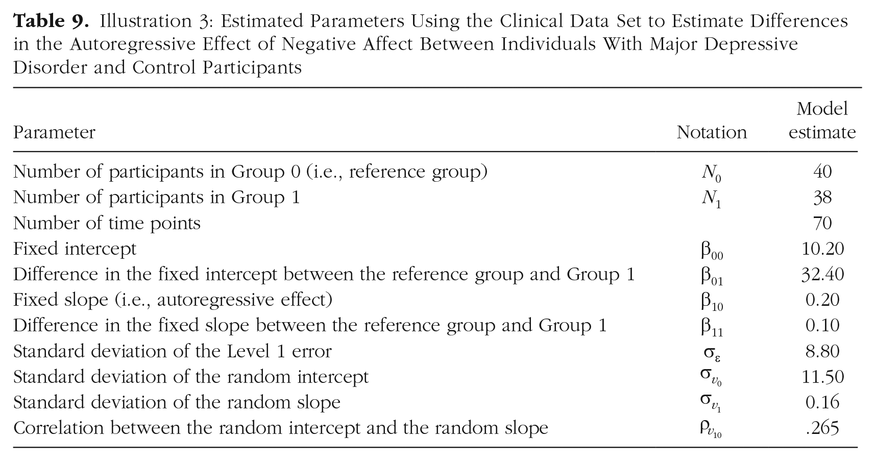
Finally, we focus on whether the autoregressive effect of negative affect differs between individuals diagnosed with MDD and control participants, and thus on Model 10. As in the previous examples, we use the clinical data set to obtain estimates of the parameter values, shown in Table 9.

Table 9.

Illustration 3: Estimated Parameters Using the Clinical Data Set to Estimate Differences in the Autoregressive Effect of Negative Affect Between Individuals With Major Depressive Disorder and Control Participants

Parameter	Notation	Model estimate
Number of participants in Group 0 (i.e., reference group)	N ₀	40
Number of participants in Group 1	N ₁	38
Number of time points		70
Fixed intercept	β₀₀	10.20
Difference in the fixed intercept between the reference group and Group 1	β₀₁	32.40
Fixed slope (i.e., autoregressive effect)	β₁₀	0.20
Difference in the fixed slope between the reference group and Group 1	β₁₁	0.10
Standard deviation of the Level 1 error	σ_ε	8.80
Standard deviation of the random intercept	$σ_{v_{0}}$	11.50
Standard deviation of the random slope	$σ_{v_{1}}$	0.16
Correlation between the random intercept and the random slope	$ρ_{v_{10}}$	.265

Step 1: app input

We select “Model 10: Multilevel AR(1) model - Group differences in the autoregressive effects.” The number of participants in the reference group (i.e., healthy control group) and the number of participants in Group 1 (i.e., MDD group) are both set to 20, 40, 60, 80, 100, 200, and 250, and the number of measurements within participants is set to 70 (see Fig. 6a). We specify the parameter values as follows (see Fig. 6b): The fixed intercept (β₀₀) is 10.20, and the difference in the fixed intercept between the two groups (β₀₁) is 32.40. The autoregressive effect (β₁₀) is 0.20. The difference in the autoregressive effect between the two groups (β₁₁) is 0.10. The standard deviation of the Level 1 errors is 8.80. The standard deviations of the random intercept and random slope are 11.50 and 0.16, respectively. The correlation between the random effects is .265. We person-mean-center the lagged outcome variable.

Fig. 6.

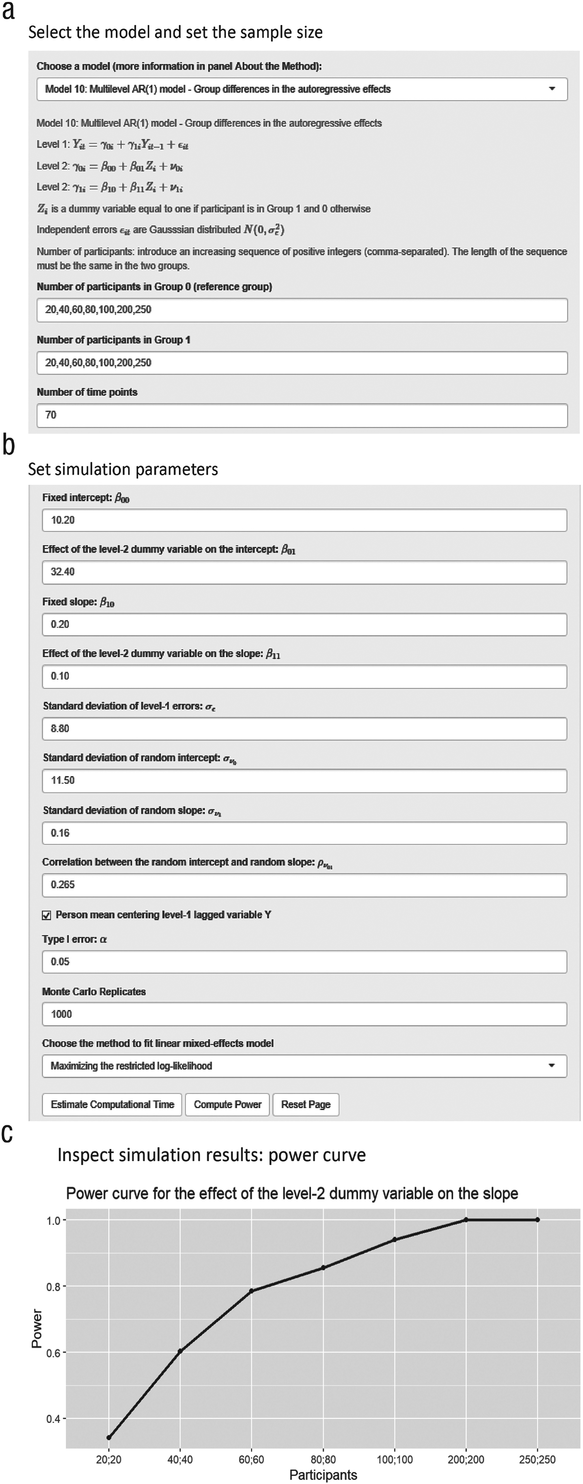
Illustration 3: differences between groups in the autoregressive effect of negative affect. These screenshots of the PowerAnalysisIL app show (a) the window in which Model 10 has been selected and the sample size has been set, (b) the values to which the parameters of the model have been set, and (c) the power curve for estimating the effect of interest.

Step 2: app output

Figure 6c shows the estimated power curve. The power to test the difference in the autoregressive effect (β₁₁) between the two groups is larger than 80% when there are 80 participants diagnosed with MDD and 80 healthy control participants. As shown in Table 10, there is a downward bias in the estimated value of the fixed slope in the reference group (β₁₀). Furthermore, when the number of participants increases, the 95% coverage proportion of the fixed slope diminishes. This is related to the bias in the estimate of the fixed slope and the narrowing of confidence intervals (i.e., smaller standard errors) when the sample size increases. This result is in line with Hamaker and Grasman’s (2015) simulations for this model, which showed that the estimated fixed slope is negatively biased when the lagged dependent variable is person-mean centered.

Table 10.

Illustration 3: Summary of Fixed Effects in the Model of Differences Between Groups in the Autoregressive Effect of Negative Affect

Effect and group size	True value	Mean	SE	Bias	(1 − α)% coverage proportion	Power
Fixed intercept
n = 20 per group	10.20	10.2638	0.0797	0.0638	.951	.979
n = 40 per group	10.20	10.2277	0.0580	0.0277	.941	.999
n = 60 per group	10.20	10.2293	0.0458	0.0293	.960	1.000
n = 80 per group	10.20	10.2027	0.0401	0.0027	.954	1.000
n = 100 per group	10.20	10.1838	0.0354	−0.0162	.960	1.000
n = 200 per group	10.20	10.1844	0.0250	−0.0156	.961	1.000
n = 250 per group	10.20	10.1978	0.0228	−0.0022	.951	1.000
Effect of the Level 2 dummy variable on the intercept
n = 20 per group	32.40	32.4069	0.1121	0.0069	.959	1.000
n = 40 per group	32.40	32.3521	0.0793	−0.0479	.962	1.000
n = 60 per group	32.40	32.3738	0.0633	−0.0262	.969	1.000
n = 80 per group	32.40	32.4743	0.0572	0.0743	.956	1.000
n = 100 per group	32.40	32.3583	0.0514	−0.0417	.948	1.000
n = 200 per group	32.40	32.3942	0.0348	−0.0058	.966	1.000
n = 250 per group	32.40	32.4214	0.0318	0.0214	.959	1.000
Fixed slope
n = 20 per group	0.20	0.1795	0.0013	−0.0205	.925	.981
n = 40 per group	0.20	0.1776	0.0010	−0.0224	.885	1.000
n = 60 per group	0.20	0.1781	0.0008	−0.0219	.846	1.000
n = 80 per group	0.20	0.1781	0.0007	−0.0219	.816	1.000
n = 100 per group	0.20	0.1776	0.0006	−0.0224	.790	1.000
n = 200 per group	0.20	0.1778	0.0004	−0.0222	.622	1.000
n = 250 per group	0.20	0.1780	0.0004	−0.0220	.551	1.000
Effect of the Level 2 dummy variable on the slope
n = 20 per group	0.10	0.0948	0.0019	−0.0052	.953	.344
n = 40 per group	0.10	0.0974	0.0014	−0.0026	.944	.612
n = 60 per group	0.10	0.0967	0.0011	−0.0033	.942	.776
n = 80 per group	0.10	0.0965	0.0010	−0.0035	.939	.873
n = 100 per group	0.10	0.0958	0.0009	−0.0042	.933	.928
n = 200 per group	0.10	0.0975	0.0006	−0.0025	.956	.999
n = 250 per group	0.10	0.0971	0.0006	−0.0029	.944	1.000

Note: This table summarizes results across 1,000 Monte Carlo replicates.

Discussion

IL designs allow studying within-person psychological dynamics. When multiple participants are included in an IL study, multilevel models are a powerful approach to capture these within-person processes as well as interindividual differences therein. When planning IL studies, it is obviously essential to collect a sufficient amount of data to ensure reliable estimates and sufficient power. In this article, we have focused on the number of participants who are needed to obtain sufficient statistical power for testing hypotheses about specific parameters of the multilevel models that are popular in IL studies. These power questions cannot be addressed by existing software for standard multilevel models, as standard models do not account for temporal dependencies in the outcome variable. Therefore, we have presented a Shiny app developed in R that uses simulation to compute power for models with an AR(1) error structure or with the lagged outcome variable as a predictor. The app yields power curves that show how estimated power varies as a function of the number of participants. In the following, we discuss limitations of the current version of the Shiny app as well as potential extensions.

Accommodating uncertainty about the hypothesized model parameters

Using simulation-based power analysis for multilevel models is challenging, in that users have to specify all the parameter values of the population model of interest. Following Lane and Hennes (2018) and Maxwell et al. (2008), we recommend basing these values on a literature review, on data from a pilot study (as we did by means of the clinical data set), or on previously conducted studies with similar measures and designs. Having said that, we acknowledge that the second and third approaches may imply that data are used from a small or unrepresentative sample, which may produce biased estimates as input for the power analysis (e.g., Albers & Lakens, 2018). Therefore, a more robust power-calculation approach would account for uncertainty regarding the hypothesized model parameters. This can be achieved by performing a sensitivity analysis in which the values of the model parameters are varied to some extent (e.g., Lane & Hennes, 2018; Y. A. Wang & Rhemtulla, 2021). This way, one can assess whether and to what extent using different possible parameter values influences the obtained power results. We note, however, that the current version of the app cannot display power curves as a function of sets of different plausible parameter values. Therefore, users have to perform a sensitivity analysis by conducting a separate power analysis for each set of parameter values.

Selecting the numbers of measurement occasions and persons

When multilevel modeling is applied to IL data, the obtained power is a function of both the number of measurement occasions and the number of participants. In this article, we have targeted the number of participants and kept the number and spacing of the measurement occasions fixed. Although this worked well for the research questions that we considered (i.e., we considered a relatively large number of measurement occasions), it is important to note that other research questions might call for increasing the number of measurement occasions. It makes sense, for instance, that when interindividual differences in within-person effects are of interest, the number of measurement occasions should be large as well. Indeed, earlier work of de Haan-Rietdijk et al. (2017), Krone et al. (2016), Liu (2017), Schultzberg and Muthén (2018), and Timmons and Preacher (2015) has demonstrated the effect that the number and spacing of the measurement occasions can have on estimation accuracy of multilevel approaches for IL data. Thus, how to best plan for adequate power depends on where power vulnerabilities are (see, e.g., Lane & Hennes, 2018).

What do users have to do when they are interested in studying not only how the number of participants affects power, but also how the number of measurement occasions affects power? Although one cannot get power curves for that from our app, a relatively simple solution consists of conducting repeated simulations with different numbers of measurement occasions while keeping the vector of sample sizes fixed. However, adding more participants or more measurements per participant may come with additional costs for researchers and may also increase participants’ burden. Therefore, researchers designing IL studies might be interested in balancing the two sample-size components to optimize power and minimize costs and participants’ burden. One way to achieve this is to obtain a set of combinations (i.e., of the number of participants and the number of measurement occasions per participant) that yield equal power and to select the combination that optimizes budgetary feasibility or other concerns. We note, however, that the current version of the app does not allow users to obtain such a set of combinations that produce equivalent power. We therefore recommend Brandmaier et al. (2015), Moerbeek (2011), and von Oertzen (2010) for a broader discussion on this topic.

Other remarks and future extensions

In the current Tutorial, we have illustrated how to use the PowerAnalysisIL app to estimate the number of participants needed for sufficient power to answer three specific research questions. For each research question, we focused on computing power for a single (fixed) effect. Yet the app also providespower curves for all other fixed effects included in a model. Therefore, in studies that involve testing multiple fixed effects, the number of participants should be large enough to detect all these effects with high power.

Even though the app is already quite extensive and includes no fewer than 11 models, many additional models could be included. For instance, in many applications, the objective is to assess the significance of the random effects. This is not possible in the current version of the app. Also, we have focused on two-levels models in which repeated measurements are nested within individuals. In the future, the proposed approach could be extended to three-level models (i.e., occasions nested within days, which in turn are nested within individuals). Three-level models are especially relevant if the dynamics under study differ systematically across days. Ignoring these differences could affect the reliability of the estimated results (de Haan-Rietdijk et al., 2016) and consequently the power.

The app simulates and analyzes data under the assumption that the measurement occasions are equally spaced and contain no missing data. In IL research, participants might not respond at some measurement occasions or during night breaks (e.g., Fuller-Tyszkiewicz et al., 2013; Santangelo et al., 2014; Stone et al., 2003). Whereas missingness might sometimes occur completely at random, in other cases it might be systematic (e.g., associated with certain affective states or certain times or contexts), which can lead to unreliable estimates (Courvoisier et al., 2012). To account for this, it would be useful to extend the simulation approach to study the effect of different types of missing data and attrition on power. For instance, when data can be assumed to be missing completely at random, users could simply specify the expected number of completed measurement occasions. Studying the effects of other mechanisms of missingness is more involved, however, because the mechanism has to be fully specified in order to simulate data.

Finally, we would like to highlight that power is not the only criterion to base sample-size selection on. Aside from maximizing the likelihood that a hypothesized effect in a population is detected, researchers might, for instance, be interested in increasing the precision of an estimate by controlling the width of the confidence interval of interest (e.g., Maxwell et al., 2008). Given that sample-size planning is important for the two related objectives of power and precision, our simulation-based approach could be extended in this direction, allowing users to additionally select the sample size that yields a targeted confidence-interval width.

Conclusion

This Tutorial has introduced a Shiny app for selecting the number of participants in IL designs. The application performs simulation-based power analysis for effects in multilevel models. We hope that the application contributes to good research practices by allowing rigorous sample-size planning for IL studies, which is of crucial importance to increase the reliability and replicability of psychological research.

Footnotes

Acknowledgements

We would like to thank our colleagues within the Research Group of Quantitative Psychology and Individual Differences and the Center for Contextual Psychiatry, particularly Leonie Cloos, for testing the app and providing useful feedback.

Transparency

Action Editor: Mijke Rhemtulla

Editor: Daniel J. Simons

Author Contributions

G. Lafit, J. K. Adolf, W. Viechtbauer, and E. Ceulemans conceptualized the application. G. Lafit, J. K. Adolf, and E. Ceulemans conceptualized the Tutorial. G. Lafit developed the Shiny app. G. Lafit and E. Dejonckheere analyzed and interpreted the clinical data set. G. Lafit, J. K. Adolf, and E. Ceulemans wrote the manuscript. E. Dejonckheere, I. Myin-Germeys, and W. Viechtbauer provided critical revisions of the manuscript and Shiny app.

ORCID iDs

Ginette Lafit

Egon Dejonckheere

Wolfgang Viechtbauer

Prior Versions

The accepted manuscript was posted online as a preprint, at .

Notes

References

Albers

Lakens

(2018). When power analyses based on pilot data are biased: Inaccurate effect size estimators and follow-up bias. Journal of Experimental Social Psychology, 74, 187–195.

Arend

M. G.

Schäfer

(2019). Statistical power in two-level models: A tutorial based on Monte Carlo simulation. Psychological Methods, 24(1), 1–19.

Astivia

O. L. O.

Gadermann

Guhn

(2019). The relationship between statistical power and predictor distribution in multilevel logistic regression: A simulation-based approach. BMC Medical Research Methodology, 19(1), 97–117.

Bates

Kliegl

Vasishth

Baayen

(2015). Parsimonious mixed models. arXiv. https://arxiv.org/pdf/1506.04967.pdf

Bolger

(2011). Power analysis for intensive longitudinal studies. In Bolger

Stadler

Laurenceau

J.-P.

(Eds.), Handbook of research methods for studying daily life (pp. 285–301). Guilford Press.

Brandmaier

A. M.

von Oertzen

Ghisletta

Hertzog

Lindenberger

(2015). LIFESPAN: A tool for the computer-aided design of longitudinal studies. Frontiers in Psychology, 6, Article 272. https://doi.org/10.3389/fpsyg.2015.00272

Brose

Schmiedek

Koval

Kuppens

(2015). Emotional inertia contributes to depressive symptoms beyond perseverative thinking. Cognition and Emotion, 29(3), 527–538.

Browne

W. J.

Lahi

M. G.

Parker

R. M.

(2009). A guide to sample size calculations for random effect models via simulation and the MLPowSim software package. https://seis.bristol.ac.uk/~frwjb/esrc/MLPOWSIMmanual.pdf

Chang

Cheng

Allaire

J. J.

Xie

McPherson

(2019). shiny: Web application framework for R (Version 1.3.2) [Computer software]. Comprehensive R Archive Network. https://CRAN.R-project.org/package=shiny

10.

Clark

(2020). Convergence problems. https://m-clark.github.io/posts/2020-03-16-convergence/

11.

Cohen

(1988). Statistical power analysis for the behavioral sciences (2nd ed.). Erlbaum.

12.

Cools

Van den Noortgate

Onghena

(2008). ML-DEs: A program for designing efficient multilevel studies. Behavior Research Methods, 40(1), 236–249.

13.

Courvoisier

D. S.

Eid

Lischetzke

(2012). Compliance to a cell phone-based ecological momentary assessment study: The effect of time and personality characteristics. Psychological Assessment, 24(3), 713–720.

14.

de Haan-Rietdijk

Kuppens

Hamaker

E. L.

(2016). What’s in a day? A guide to decomposing the variance in intensive longitudinal data. Frontiers in Psychology, 7, Article 891. https://doi.org/10.3389/fpsyg.2016.00891

15.

de Haan-Rietdijk

Voelkle

M. C.

Keijsers

Hamaker

E. L.

(2017). Discrete- vs. continuous-time modeling of unequally spaced experience sampling method data. Frontiers in Psychology, 8, Article 1849. https://doi.org/10.3389/fpsyg.2017.01849

16.

Dejonckheere

Mestdagh

Houben

Erbas

Koval

Brose

Bastian

Kuppens

(2018). The bipolarity of affect and depressive symptoms. Journal of Personality and Social Psychology, 114(2), 323–341.

17.

De Jong

Moerbeek

Van der Leeden

(2010). A priori power analysis in longitudinal three-level multilevel models: An example with therapist effects. Psychotherapy Research, 20(3), 273–284.

18.

Enders

C. K.

Tofighi

(2007). Centering predictor variables in cross-sectional multilevel models: A new look at an old issue. Psychological Methods, 12(2), 121–138.

19.

Fuller-Tyszkiewicz

Skouteris

Richardson

Blore

Holmes

Mills

(2013). Does the burden of the experience sampling method undermine data quality in state body image research? Body Image, 10(4), 607–613.

20.

Goldstein

Healy

M. J.

Rasbash

(1994). Multilevel time series models with applications to repeated measures data. Statistics in Medicine, 13(16), 1643–1655.

21.

Green

MacLeod

C. J.

(2016). SIMR: An R package for power analysis of generalized linear mixed models by simulation. Methods in Ecology and Evolution, 7(4), 493–498.

22.

Hamaker

E. L.

Grasman

R. P. P. P.

(2015). To center or not to center? Investigating inertia with a multilevel autoregressive model. Frontiers in Psychology, 5, Article 1492. https://doi.org/10.3389/fpsyg.2014.01492

23.

Hamaker

E. L.

Kuiper

R. M.

Grasman

R. P.

(2015). A critique of the cross-lagged panel model. Psychological Methods, 20(1), 102–116.

24.

Hamilton

J. D.

(1994). Time series analysis. Princeton University Press.

25.

Hedeker

Gibbons

R. D.

Waternaux

(1999). Sample size estimation for longitudinal designs with attrition: Comparing time-related contrasts between two groups. Journal of Educational and Behavioral Statistics, 24(1), 70–93.

26.

Heininga

V. E.

Dejonckheere

Houben

Obbels

Sienaert

Leroy

van Roy

Kuppens

(2019). The dynamical signature of anhedonia in major depressive disorder: Positive emotion dynamics, reactivity, and recovery. BMC Psychiatry, 19(1), Article 59. https://doi.org/10.1186/s12888-018-1983-5

27.

Ioannidis

J. P. A.

(2005). Why most published research findings are false. PLOS Medicine, 2(8), Article e124. https://doi.org/10.1371/journal.pmed.0020124

28.

Kirtley

O. J.

Lafit

Achterhof

Hiekkaranta

A. P.

Myin-Germeys

(in press). Making the black box transparent: A template and tutorial for registration of studies using experience-sampling methods. Advances in Methods and Practices in Psychological Science.

29.

Koval

M. L.

Meers

Kuppens

(2013). Affect dynamics in relation to depressive symptoms: Variable, unstable or inert? Emotion, 13(6), 1132–1141.

30.

Krone

Albers

C. J.

Timmerman

M. E.

(2016). Comparison of estimation procedures for multilevel AR(1) models. Frontiers in Psychology, 7, Article 486. https://doi.org/10.3389/fpsyg.2016.00486

31.

Kuppens

Allen

N. B.

Sheeber

L. B.

(2010). Emotional inertia and psychological maladjustment. Psychological Science, 21(7), 984–991.

32.

Kuppens

Verduyn

(2015). Looking at emotion regulation through the window of emotion dynamics. Psychological Inquiry, 26(1), 72–79.

33.

Landau

Stahl

(2013). Sample size and power calculations for medical studies by simulation when closed form expressions are not available. Statistical Methods in Medical Research, 22(3), 324–345.

34.

Lane

S. P.

Hennes

E. P.

(2018). Power struggles: Estimating sample size for multilevel relationships research. Journal of Social and Personal Relationships, 35(1), 7–31.

35.

Liu

(2017). Person-specific versus multilevel autoregressive models: Accuracy in parameter estimates at the population and individual levels. British Journal of Mathematical and Statistical Psychology, 70(3), 480–498.

36.

Maas

C. J.

Hox

J. J.

(2005). Sufficient sample sizes for multilevel modeling. Methodology: European Journal of Research Methods for the Behavioral and Social Sciences, 1(3), 86–92.

37.

Mathieu

J. E.

Aguinis

Culpepper

S. A.

Chen

(2012). Understanding and estimating the power to detect cross-level interaction effects in multilevel modeling. Journal of Applied Psychology, 97(5), 951–966.

38.

Maxwell

S. E.

Kelley

Rausch

J. R.

(2008). Sample size planning for statistical power and accuracy in parameter estimation. Annual Review of Psychology, 59, 537–563.

39.

Moerbeek

(2011). The effects of the number of cohorts, degree of overlap among cohorts, and frequency of observation on power in accelerated longitudinal designs. Methodology: European Journal of Research Methods for the Behavioral and Social Sciences, 7(1), 11–24.

40.

Moerbeek

Maas

C. J.

(2005). Optimal experimental designs for multilevel logistic models with two binary predictors. Communications in Statistics—Theory and Methods, 34(5), 1151–1167.

41.

Moerbeek

van Breukelen

G. J. P.

Berger

M. P. F.

(2000). Design issues for experiments in multilevel populations. Journal of Educational and Behavioral Statistics, 25(3), 271–284.

42.

Moerbeek

Van Breukelen

G. J. P.

Berger

M. P. F.

(2001). Optimal experimental designs for multilevel logistic models. Journal of the Royal Statistical Society: Series D (The Statistician), 50(1), 17–30.

43.

Molenaar

P. C.

(2004). A manifesto on psychology as idiographic science: Bringing the person back into scientific psychology, this time forever. Measurement, 2(4), 201–218.

44.

Morris

T. P.

White

I. R.

Crowther

M. J.

(2019). Using simulation studies to evaluate statistical methods. Statistics in Medicine, 38(11), 2074–2102.

45.

Munafò

M. R.

Nosek

B. A.

Bishop

D. V. M.

Button

K. S.

Chambers

C. D.

Percie

Sert

Simonsohn

Wagenmakers

E.-J.

Ware

J. J.

Ioannidis

J. P. A.

(2017). A manifesto for reproducible science. Nature Human Behaviour, 1(1), Article 0021. https://doi.org/10.1038/s41562-016-0021

46.

Myin-Germeys

Kasanova

Vaessen

Vachon

Kirtley

Viechtbauer

Reininghaus

(2018). Experience sampling methodology in mental health research: New insights and technical developments. World Psychiatry, 17(2), 123–132.

47.

Myin-Germeys

Oorschot

Collip

Lataster

Delespaul

van Os

(2009). Experience sampling research in psychopathology: Opening the black box of daily life. Psychological Medicine, 39(9), 1533–1547.

48.

Myin-Germeys

Peeters

Havermans

Nicolson

N. A.

DeVries

M. W.

Delespaul

Van Os

(2003). Emotional reactivity to daily life stress in psychosis and affective disorder: An experience sampling study. Acta Psychiatrica Scandinavica, 107(2), 124–131.

49.

Myin-Germeys

van Os

Schwartz

J. E.

Stone

A. A.

Delespaul

P. A.

(2001). Emotional reactivity to daily life stress in psychosis. Archives of General Psychiatry, 58(12), 1137–1144.

50.

Pinheiro

Bates

DebRoy

Sarkar

, & R Core Team. (2019). nlme: Linear and nonlinear mixed effects mdels (Version 3.1-141) [Computer software]. Comprehensive R Archive Network. https://cran.r-project.org/web/packages/nlme/index.html

51.

R Core Team. (2020). R: A language and environment for statistical computing (Version 4.0.3) [Computer software]. R Foundation for Statistical Computing. https://www.R-project.org/

52.

Raudenbush

S. W.

(1997). Statistical analysis and optimal design for cluster randomized trials. Psychological Methods, 2(2), 173–185.

53.

Raudenbush

S. W.

Bryk

A. S.

(2002). Hierarchical linear models: Applications and data analysis methods (2nd ed.). Sage.

54.

Raudenbush

S. W.

Liu

X.-F.

(2001). Effects of study duration, frequency of observation, and sample size on power in studies of group differences in polynomial change. Psychological Methods, 6(4), 387–401.

55.

RStudio Team. (2015). RStudio: Integrated Development Environment for R. RStudio, Inc.

56.

Rush

A. J.

Trivedi

M. H.

Ibrahim

H. M.

Carmody

T. J.

Arnow

Klein

D. N.

Markowitz

J. C.

Ninan

P. T.

Kornstein

Manber

Thase

M. E.

Kocsis

J. H.

Keller

M.B.

(2003). The 16-item Quick Inventory of Depressive Symptomatology (QIDS), clinician rating (QIDS-C), and self-report (QIDS-SR): A psychometric evaluation in patients with chronic major depression. Biological Psychiatry, 54(5), 573–583.

57.

Santangelo

Bohus

Ebner-Priemer

U. W.

(2014). Ecological momentary assessment in borderline personality disorder: A review of recent findings and methodological challenges. Journal of Personality Disorders, 28(4), 555–576.

58.

Schultzberg

Muthén

(2018). Number of subjects and time points needed for multilevel time-series analysis: A simulation study of dynamic structural equation modeling. Structural Equation Modeling: A Multidisciplinary Journal, 25(4), 495–515.

59.

Snijders

T. A.

Bosker

R. J.

(1993). Standard errors and sample sizes for two-level research. Journal of Educational Statistics, 18(3), 237–259.

60.

Snijders

T. A.

Bosker

R. J.

(2011). Multilevel analysis: An introduction to basic and advanced multilevel modeling. SAGE Publications.

61.

Stone

A. A.

Broderick

J. E.

Schwartz

J. E.

Shiffman

Litcher-Kelly

Calvanese

(2003). Intensive momentary reporting of pain with an electronic diary: Reactivity, compliance, and patient satisfaction. Pain, 104(1–2), 343–351.

62.

Szucs

Ioannidis

J. P. A.

(2017). Empirical assessment of published effect sizes and power in the recent cognitive neuroscience and psychology literature. PLOS Biology, 15(3), Article e2000797. https://doi.org/10.1371/journal.pbio.2000797

63.

Timmons

A. C.

Preacher

K. J.

(2015). The importance of temporal design: How do measurement intervals affect the accuracy and efficiency of parameter estimates in longitudinal research? Multivariate Behavioral Research, 50(1), 41–55.

64.

Trull

T. J.

Ebner-Priemer

U. W.

(2020). Ambulatory assessment in psychopathology research: A review of recommended reporting guidelines and current practices. Journal of Abnormal Psychology, 129(1), 56–63.

65.

von Oertzen

(2010). Power equivalence in structural equation modelling. British Journal of Mathematical and Statistical Psychology, 63(2), 257–272.

66.

Wang

Hall

C. B.

Kim

(2015). A comparison of power analysis methods for evaluating effects of a predictor on slopes in longitudinal designs with missing data. Statistical Methods in Medical Research, 24(6), 1009–1029.

67.

Wang

L. P.

Hamaker

Bergeman

(2012). Investigating inter-individual differences in short-term intra-individual variability. Psychological Methods, 17(4), 567–581.

68.

Wang

Y. A.

Rhemtulla

(2021). Power analysis for parameter estimation in structural equation modeling: A discussion and tutorial. Advances in Methods and Practices in Psychological Science, 4(1). https://doi.org/10.1177/2515245920918253

69.

Zhang

(2014). Monte Carlo based statistical power analysis for mediation models: Methods and software. Behavior Research Methods, 46(4), 1184–1198.

70.

Zhang

Wang

(2009). Statistical power analysis for growth curve models using SAS. Behavior Research Methods, 41(4), 1083–1094.

Selection of the Number of Participants in Intensive Longitudinal Studies: A User-Friendly Shiny App and Tutorial for Performing Power Analysis in Multilevel Regression Models That Account for Temporal Dependencies

Abstract

Keywords

Disclosures

Power Analyses in Intensive Longitudinal Studies

Population Models of Interest

Group differences in mean level

Effect of a Level 2 continuous predictor on the mean level

Effect of a Level 1 continuous predictor

Group differences in the effect of a Level 1 continuous predictor

Cross-level interaction between two continuous predictors

Multilevel autoregressive models

A Shiny App to Perform Power Analysis

App input

Simulation

App output

Illustrations

Data set

Illustration 1: power to estimate the effect of a Level 2 predictor

Step 1: app input

Step 2: app output

Illustration 2: power to detect the effect of a Level 1 predictor

Step 1: app input

Step 2: app output

Illustration 3: power to detect the differences in the autoregressive effects between two groups

Step 1: app input

Step 2: app output

Discussion

Accommodating uncertainty about the hypothesized model parameters

Selecting the numbers of measurement occasions and persons

Other remarks and future extensions

Conclusion

Footnotes

Acknowledgements

Transparency

ORCID iDs

Prior Versions

Notes

References