A Traveler’s Guide to the Multiverse: Promises,Pitfalls,and a Framework for the Evaluation of Analytic Decisions

Abstract

Decisions made by researchers while analyzing data (e.g., how to measure variables, how to handle outliers) are sometimes arbitrary, without an objective justification for choosing one alternative over another. Multiverse-style methods (e.g., specification curve, vibration of effects) estimate an effect across an entire set of possible specifications to expose the impact of hidden degrees of freedom and/or obtain robust, less biased estimates of the effect of interest. However, if specifications are not truly arbitrary, multiverse-style analyses can produce misleading results, potentially hiding meaningful effects within a mass of poorly justified alternatives. So far, a key question has received scant attention: How does one decide whether alternatives are arbitrary? We offer a framework and conceptual tools for doing so. We discuss three kinds of a priori nonequivalence among alternatives—measurement nonequivalence, effect nonequivalence, and power/precision nonequivalence. The criteria we review lead to three decision scenarios: Type E decisions (principled equivalence), Type N decisions (principled nonequivalence), and Type U decisions (uncertainty). In uncertain scenarios, multiverse-style analysis should be conducted in a deliberately exploratory fashion. The framework is discussed with reference to published examples and illustrated with the help of a simulated data set. Our framework will help researchers reap the benefits of multiverse-style methods while avoiding their pitfalls.

Recently introduced in the form of multiverse analysis (Steegen et al., 2016), specification-curve analysis (Simonsohn et al., 2018, 2020), assessment of vibration of effects (VoE; Patel et al., 2015), and similar approaches (e.g., Young & Kindzierski, 2019), multiverse-style methods have quickly attracted attention. In standard practice, researchers report one analysis or, at most, a small subset of all possible analyses of their data set. These analyses may not be representative of the entire set of possibilities, and their results may be biased by the selective use of hidden degrees of freedom. In multiverse-style methods, researchers explicitly specify the decision nodes required to prepare a data set for analysis. These decision nodes are used to generate all possible combinations of decisions, and the data are analyzed using the full array of specifications.

The potential of multiverse-style methods is obvious; it is hard to overstate the importance of reporting analytic decisions transparently and exploring the robustness of research findings. At the same time, we see some pressing reasons for concern. The central notion of these methods is that the alternatives included in the multiverse are “arbitrary” or equally “reasonable.” However, there is little guidance or consensus on how to evaluate arbitrariness, and virtually no consideration of the potential pitfalls of multiverse-style methods. What are the implications if some of the choices regarded as arbitrary are in fact not? We feel that researchers have started traveling across the multiverse without a map, and often with surprisingly little awareness of the dangers that lurk out there. In this article, we address these issues and offer an initial map to the multiverse, in the form of a systematic framework for the evaluation of analytic decisions.

Multiverse-Style Methods: Rationale, Promises, and Pitfalls

When they perform data analysis, researchers must make decisions—for example which predictor and criterion variables to examine, whether to aggregate measures, and what exclusion criteria, if any, should be applied to individual cases. Researchers typically report a single analysis or, at most, a few analyses and results; these analyses may or may not be representative of the multiverse of possible valid specifications. This is true even if the analytic plan for the study was preregistered: Although preregistration limits the scope for p-hacking and similar questionable practices, it does not guarantee that the chosen specifications are representative and robust (Steegen et al., 2016).

A way to address this problem is to systematically generate a set of alternative specifications and examine the aggregate results, for example, by plotting the resulting distribution of p values (Steegen et al., 2016) or a detailed specification curve (Simonsohn et al., 2018, 2020). In principle, one can perform traditional hypothesis tests on results from all specifications through randomization or bootstrapping (see Simonsohn et al., 2020). Similarly, in an assessment of the VoE, one plots the results as a scatterplot of p values as a function of effect sizes and computes summary statistics reflecting the variability of effects (Patel et al., 2015).

Arbitrariness and the multiverse

As Steegen et al. (2016) explicitly discussed, “the practice of selective reporting would not be problematic if the single data set under consideration is processed based on sound and justifiable choices” (p. 703). But “choosing among the alternatives is often arbitrary, and justifications for the choices are typically lacking” (p. 703). The multiverse is constructed from these arbitrary choices, such that, on a priori grounds, no particular analysis within the multiverse is more justifiable than any other. Similarly, within specification-curve analysis, researchers examine all “reasonable” specifications (Simonsohn et al., 2018, 2020).

These stances raise a critical issue: What does it mean for alternative options to be arbitrary, as opposed to one option being justified and reasonable relative to others? Steegen et al. (2016) offered very little guidance in this regard. Simonsohn et al. (2018, 2020) noted that arbitrary decisions are, at least in part, ones for which theory offers very little justification. By contrast, any choice that theory or background knowledge indicates is clearly justified over others is nonarbitrary and should not be used to generate alternative specifications. Simonsohn et al. (2020) also stressed that investigators should not consider specifications that are “unambiguously inferior” (p. 1209) to alternatives. These considerations are crucially important, and the motivation behind our own analysis in this article. Yet Simonsohn et al. did not substantiate their remarks with an in-depth examination of why certain specifications may be objectively preferable to others. Accordingly, multiverse-style analyses published to date have rarely been accompanied by any detailed discussion of why and how certain decisions were deemed arbitrary (e.g., Hall et al., 2019; Hässler et al., 2019; Moors & Hesselmann, 2019; Orben et al., 2019; Orben & Przybylski, 2019a, 2019b, 2020; Rae et al., 2019; Rohrer et al., 2017; Stamos et al., 2020; Stern et al., 2019).

The absence of consensus in the literature extends to basic analytic issues such as covariate selection. Simonsohn et al. (2018) correctly stressed that analyses “with and without a certain set of covariates are not different answers to the same question, they are different answers to different questions” (p. 10). Decisions of which covariates to include, then, “should not usually be part of robustness tests” (p. 10). ¹ In striking contrast, Patel et al. (2015) demonstrated the VoE with robustness analyses that involved only alternative sets of covariates. This and other examples reveal a pressing need for conceptual clarity and suggest that the absence of reasoned guidelines has limited the potential of multiverse-style methods in practical applications.

The multiverse is a dangerous place

In principle, multiverse-style analyses can be highly instructive. At the same time, analyses that explore multiverse spaces that are not homogeneous can produce misleading results and interpretations, lead scholars to dismiss the robustness of theoretically important findings that do exist, and discourage them from following fruitful avenues of research. This can hinder scientific progress just as much as the proliferation of false, unreplicable findings does (see Fiedler, 2018; Fiedler et al., 2012).

The main danger of multiverse-style methods lies in their potential for combinatorial explosion. Just a few decisions incorrectly treated as arbitrary can quickly explode the size of the multiverse, drowning reasonable effect estimates in a sea of unjustified alternatives. A single decision node with two alternatives doubles the number of specifications. Five binary decision nodes expand the multiverse by a factor of 32. If one alternative is justifiable over the other in each case, the region defined by justified choices ends up occupying just 3% of the total multiverse. If the decision nodes involve three alternatives each, the corresponding figure is 0.4%. With so many individual effects within the multiverse, researchers may find it easier to characterize the distribution of effects with simple summary statistics, such as a median or mean effect size. But when the proportion of effects that best estimate the effect of interest is very small, the central tendency of effects can become misleading or virtually meaningless.

By inflating the size of the analysis space, the combinatorial explosion of unjustified specifications may, ironically, exaggerate the perceived exhaustiveness and authoritativeness of the multiverse while greatly reducing the informative fraction of the multiverse. At the same time, the size of the specification space can make it harder to inspect the results for potentially relevant findings. If unchecked, multiverse-style analyses can generate analytic “black holes”: massive analyses that swallow true effects of interest but, because of their perceived exhaustiveness and sheer size, trap whatever information is present in impenetrable displays and summaries.

Disclosures

All the code and simulated data employed in this article are available on figshare at https://doi.org/10.6084/m9.figshare.12089736. The Supplemental Material (http://journals.sagepub.com/doi/suppl/10.1177/2515245920954925) includes a section on the reliability of composite measures (S1), a section on the problems with simultaneous entry of multiple indicators in regression models (S2), a primer on covariate selection from the standpoint of causal modeling (S3), and the results of 500 replicates of the main analysis described in the article (S4).

Mapping the Multiverse: A Framework for the Evaluation of Analytic Decisions

The key step toward a systematic evaluation of decisions is to move beyond intuitive notions of what constitutes an arbitrary or justified alternative. We now present a framework that enables this kind of evaluation, drawing on concepts from statistical inference, psychometrics, and causal modeling. We first review three distinct ways in which alternative specifications may be expected a priori to yield different answers, and thus cannot be treated as arbitrary. Specifically, we consider measurement nonequivalence, effect nonequivalence, and power/precision nonequivalence. (Note that although these kinds of nonequivalence cover many common scenarios, they are not exhaustive; other relevant domains include criteria for outliers, variable transformations, choice of statistical models, and so forth.)

We then go on to describe three types of decision scenarios. In Type E decisions (principled equivalence), the alternative specifications can be expected to be practically equivalent, and choices among them can be regarded as effectively arbitrary. In Type N decisions (principled nonequivalence), the alternative specifications are nonequivalent according to one or more nonequivalence criteria. As a result, some of the alternatives can be regarded as objectively more reasonable or better justified than the others. Finally, in Type U decisions (uncertainty), there are no compelling reasons to expect equivalence or nonequivalence, or there are reasons to suspect nonequivalence but not enough information to specify which alternatives are better justified. In this scenario, multiverse-style analyses should be carried out with a deliberately exploratory approach.

Three kinds of nonequivalence

Measurement nonequivalence

In many cases, scientific constructs are not univocally defined by a single indicator; constructs may be tapped by multiple indicators, each serving as an imperfect measure. If a construct has been measured in multiple ways within a single study, or could have been plausibly measured in alternative ways, the choice of measure becomes a node in the decision tree and may be explored in a multiverse. The problem is that different measurement choices can often be expected to yield systematic differences in validity and reliability, with predictable consequences on the effect of interest. In such cases, alternative measures cannot be treated as equivalent.

Validity and reliability

The validity of a measure is the extent to which it reflects the construct it is purported to measure. Reliability is the proportion of variance in a measure that can be regarded as signal rather than noise—in the language of classic test theory, this corresponds to the squared correlation between the observed score and the underlying true score (see Revelle & Condon, 2018). It is generally assumed that all valid variance is reliable, such that reliability puts a ceiling on validity, but some reliable variance may not be valid.

A simple way to quantify the validity of a measure is to estimate its validity coefficient, or its correlation with the construct it taps (see Fig. 1). In some cases, a perfect criterion of the construct can be assessed, such that a validity study can directly estimate this strength of association. In other cases, a validity coefficient can be estimated from simulations (e.g., Gangestad et al., 2016). If all the reliable variance in a measure is valid, the validity coefficient is just the square root of the measure’s reliability. For an overview of methods for estimating reliability, see Revelle (2015; Revelle & Condon, 2018).

Fig. 1.

Schematic illustration of a latent construct X measured with four indicators. The validity coefficient of each indicator is the correlation between the indicator and the latent construct. The diagrams illustrate cases in which (a) all the indicators have the same validity, (b) one indicator has higher validity than the rest, and (c) two putative indicators have zero validity (no association with the construct; indicated by the dashed lines).

Composite measures

Instead of individual indicators, researchers sometimes use composite measures, typically weighted or unweighted sums of multiple indicators. Component scores obtained via principal components analysis and factor scores derived from exploratory factor analysis fall in this category. Composite measures of a construct are usually more valid and reliable than individual indicators (see Section S1 of the Supplemental Material for relevant formulas). Suppose each of four indicators of a construct has a validity coefficient of .60, and thus a reliability of .36 (as in Fig. 1a). Their composite would have a validity of .83 and a reliability of .69. Even if one of the indicators is considerably more valid and reliable than the others, a composite may still yield improved performance. In the example of Figure 1b, one indicator has a validity of .80 and a reliability of .64, while the remaining ones have a validity of .50 and a reliability of .25. An equal-weighted sum of the four indicators will yield a validity of .82 and a reliability of .67. Naturally, a composite need not outperform individual indicators if some of the indicators have little to no validity. In Figure 1c, two indicators have a validity of .60, while the remaining two have zero validity. In this case, the validity of the composite of all four is .55.

The implications for multiverse-style analyses involving composite measures are twofold. First, unless the composite includes a considerable proportion of invalid indicators, it will generally yield a higher validity than individual indicators—which translates into larger effect sizes, more precise estimates, and higher statistical power. Second, if some of the indicators are known to be invalid, composites that exclude them will predictably yield higher validities than composites that include them.

In one study, the authors sought to measure children’s gender identity with a composite of five indicators—such as preference for male versus female peers, toy preference, and clothing preference (Rae et al., 2019). They then ran a multiverse analysis in which indicators were used as predictors individually and in all their possible combinations. Predictably, composites that included more indicators tended to yield larger effect sizes and/or more precise estimates of the effects.

In another study, investigators examined women’s preferences for muscular bodily features in men (Stern et al., 2019). They measured five putative cues of upper-body strength, such as shoulder-to-hip ratio and upper-arm circumference. In fact, however, just two of the cues independently predicted a criterion of muscularity (ratings of bodily dominance) of the same stimuli (Gangestad et al., 2019b). Within a multiverse analysis, the two features showing independent evidence of validity predictably outperformed the other features in predicting women’s preferences. A composite of just these features yielded even larger effect sizes (see Gangestad et al., 2019a, 2019b).

In their analysis of adolescents’ well-being and use of digital technology, Orben and Przybylski (2019a) measured well-being with the mean of any combination of items drawn from full-scale questionnaires, plus single items. One of these measures has 25 items and an internal-consistency reliability of about .80 (Stone et al., 2010). Accordingly, the expected reliability of single items and combinations of two, three, and four items drawn from the full questionnaire can be estimated at about .14, .24, .32, and .39, respectively (see Section S1 of the Supplemental Material). These shortened measures are highly unreliable, but the authors used more than 15,000 of them to populate the multiverse. (We note that in analyses on other dependent variables, these same authors used only full scales; Orben & Przybylski, 2019b.)

Simultaneous entry

When multiple indicators of a construct are available, investigators running a multiverse-style analysis may decide to enter them simultaneously as predictors—for instance, in a regression model—and test the unique effects of different combinations of predictors on a response variable. In their study of women’s preferences for bodily features, for example, Stern et al. (2019) considered seven putative indicators of bodily masculinity. In addition to examining effects of single indicators and composites, they examined effects of each indicator within a regression analysis that simultaneously entered the six remaining indicators.

This approach is problematic because the simultaneous inclusion of multiple indicators can substantially deflate the individual effect of each indicator (and reduce the corresponding statistical power). When multiple indicators partly tap the same construct, the correlation between each indicator and the construct, with all other indicators controlled for—that is, the partial validity coefficient—is necessarily less than the original validity. Notably, reductions in validity are even greater if individual indicators have larger validity coefficients, as partialing removes greater amounts of valid variance. For more details on the implications of simultaneous entry, see Section S2 of the Supplemental Material.

Effect nonequivalence

The logic of multiverse-style methods rests on the assumption that the effect of interest remains the same across the specifications included in a single analysis. Gross violations of this assumption occur when researchers include qualitatively different effects within the same analysis. For example, Stern et al. (2019) ran a single multiverse analysis that included both two-way and three-way interactions among predictors, even though the two types of effects are statistically orthogonal and pertain to substantively different empirical hypotheses (see Gangestad et al., 2019a).

More subtly but no less importantly, when alternative analyses include different sets of covariates, the effects they test often cease to be logically and/or statistically equivalent. In particular, adjusting for certain covariates may predictably add bias to (or remove bias from) the estimate of the effect of interest. The impact of including versus excluding a given variable depends on the role played by that variable in the causal model that (explicitly or implicitly) underlies the analysis (Pearl, 2009; Pearl et al., 2016; Rohrer, 2018). This is why covariate selection is fundamentally a theoretical problem, and why Simonsohn et al. (2018) advised against including alternative sets of covariates within a single multiverse.

We illustrate the importance of causal assumptions with Figure 2a, which introduces a toy model representing a fictional study of the effect of inflammation on depression. Inflammation is measured indirectly with four biomarkers, labeled BM1 through BM4. The study variables also include age, pain, fatigue, and a measure of pro-inflammatory genotype. The figure depicts the hypothesized causal relations among the variables, in the form of a directed acyclic graph (DAG; see Elwert, 2013; Pearl et al., 2016; Rohrer, 2018). According to the model, inflammation affects depression via two distinct pathways, one direct and one mediated by pain. Age affects both inflammation and depression, thus acting as a confounder of their causal relationship. If the role played by a variable can be specified with a causal model like that in Figure 2a, one can predict in advance whether including it as a covariate will add or remove estimation bias, and thus decide which alternative specification is better justified.

Fig. 2.

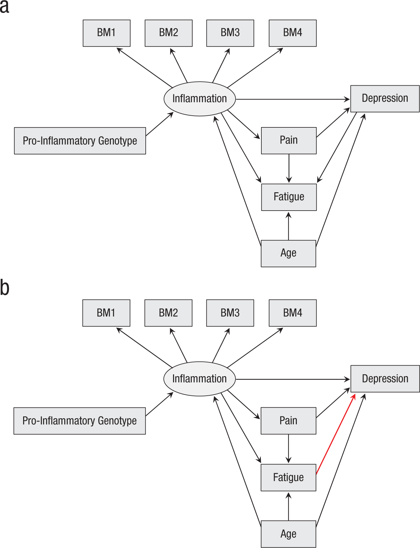
Two causal models of a hypothetical study of the effect of inflammation on depression. Rectangles indicate observed variables; ellipses indicate unobserved latent constructs. The only difference between the two models is the direction of the path from fatigue to depression (red arrow in the bottom diagram).

In Section S3 of the Supplemental Material, we provide a primer on covariate selection from the standpoint of causal analysis. For more information, we recommend the accessible book by Pearl and Mackenzie (2018) and the more advanced treatment in Pearl (2009; see also Pearl et al., 2016). Also, Rohrer (2018) offers an excellent summary of the main concepts. DAGitty (http://dagitty.net) is a useful tool that can be used to analyze causal models and explore the effects of controlling for different covariates (Textor, 2016). An interactive version of the model in Figure 2a is available at http://dagitty.net/dags.html?id=Xw8N-D.

In some cases, researchers have enough background information to specify a single model of the causal relations among the study variables. Other times, the correct causal model is unknown, or there is more than one plausible alternative. For example, Figure 2b shows a hypothetical alternative to the model of Figure 2a. Here, fatigue partially mediates the effect of inflammation on depression (as opposed to being a common effect of inflammation and depression). An interactive version of this model can be explored at http://dagitty.net/dags.html?id=X2ShVE.

According to the model in Figure 2a, fatigue is a collider and should not be included as a covariate (Rohrer, 2018; see Section S3 of the Supplemental Material). But if the model in Figure 2b is correct, fatigue is not a collider but a mediator; as such, it should be excluded if the focal hypothesis concerns the total effect of inflammation on depression, but controlled for if the hypothesis concerns the direct effect of inflammation on depression. As these specifications assess different effects and imply incompatible causal assumptions, including both in the same multiverse would be highly problematic. Note that the choice between alternative causal models does not have to rely exclusively on assumptions and preexisting information. Different models often make different predictions about the conditional relations among certain variables, which in principle makes them empirically testable against the data (see Elwert, 2013). The DAGitty website lists all the testable implications that can be derived from a given causal model.

We argue that when there is genuine uncertainty about the underlying causal model, the uncertainty should be acknowledged and addressed from a theoretically informed standpoint. In the article introducing the VoE method, Patel et al. (2015) tested several predictors of all-cause mortality while controlling for all possible combinations of 13 covariates—including heart disease, diabetes, drinking, and physical activity. Depending on the specific predictor investigated, these variables may plausibly act as either mediators or confounders of the effect. If they are mediators, the decision to include or exclude them should depend on whether direct or total effects are the focus of interest (see Section S3 of the Supplemental Material). If they are confounders, models that do not include them as covariates return biased estimates. Either way, it is entirely expected that estimated effects will change (even dramatically) when these variables are controlled for, and such changes should not be regarded as a sign of instability.

Power/precision nonequivalence

Even if the alternative specifications within a multiverse address the same effect, they may yield predictably different results if they differ in the power to detect that effect or in the precision of its estimates. This can happen when measures have different validities or reliabilities. It can also happen when alternative criteria for the inclusion/exclusion of data points (e.g., removal of outliers) result in substantially different sample sizes across specifications. For instance, Stamos et al. (2020) examined the association between socioeconomic status and generosity in a laboratory game and applied multiple exclusion criteria to the main study variables. Resulting sample sizes ranged from 114 to 300. Or consider the study by Palpacuer et al. (2019), who calculated the VoE in a series of 9,216 meta-analyses comparing the efficacy of two drugs. As a result of alternative inclusion criteria, the number of studies included ranged from five to 42 across meta-analyses. Such large differences in the size of the study set must have dramatically affected the precision of the estimates, but this important factor was not discussed in the report.

Less intuitively, including certain covariates in the statistical model can increase or decrease the precision of the estimated effect, even if those covariates have no effect on estimation bias (Cinelli et al., 2019; Pearl et al., 2016). We briefly discuss this phenomenon in Section S3 of the Supplemental Material.

Three types of analytic decisions

Type E decisions: principled equivalence

For a particular decision node, evidence and conceptual considerations may indicate that alternative analyses are effectively equivalent: Alternative measures have comparable validity, alternative analyses examine the same effect, and the parameter of interest is estimated with comparable precision or power. If so, results arising from alternative specifications should differ only for nonsubstantive reasons (sampling variability, quirks of the data, and so on). Type E decisions imply true arbitrariness and are properly used to populate a homogeneous multiverse.

Naturally, only rarely will, say, two different measures have precisely the same validity. But the evidence may indicate that the validities are similar enough to make no practical difference. If in doubt, one can use simulations to assess how similar alternative specifications need to be to make no important difference to the conclusions of the analysis.

Type N decisions: principled nonequivalence

At times, the available evidence and other considerations support the conclusion that alternative specifications are not equivalent, and some are objectively more justified than others as a means of estimating the effect of interest. A Type N decision implies that alternatives are not arbitrary, and hence should not be used to populate a single multiverse. Often, there is little reason to explore the less preferable alternatives, because they are expected a priori to yield deflated effects, biased effects, or estimates suffering from low power and/or precision. If, however, researchers are interested in exploring those alternatives (e.g., to compare the direct vs. total effect of a predictor), they should do so in separate analyses to avoid confounding the results.

Type U decisions: uncertainty

In some instances, there are no compelling reasons to expect equivalence or nonequivalence, or there is reason to expect nonequivalence, but insufficient information to specify which alternatives are better justified. For example, a researcher may have alternative measures of a construct (say, a questionnaire and a behavioral observation); though these measures are different enough that they are unlikely to have comparable validity, there may be no empirical evidence revealing which measure is more valid. In other cases, reasonable uncertainty about the causal model underlying the data may generate uncertainty about the inclusion or exclusion of covariates, as illustrated by the toy models in Figures 2a and 2b: If there is no clear reason to prefer one causal model over the other, including or excluding fatigue is a Type U decision.

Researchers may be tempted to treat Type U decisions similarly to how they treat Type E decisions, but, in fact, the implications for the multiverse are very different. In one case, alternatives are truly arbitrary, and choosing one over another should not matter (i.e., should not yield different results). In the other case, choosing one over the other does matter, even if there is insufficient knowledge to determine a priori which alternatives are better justified. When facing Type U decisions, it can be profitable to carry out multiverse-style analyses as a deliberately exploratory endeavor, in which alternatives are examined separately (see also Simonsohn et al., 2018, for relevant discussion).

A broader view of transparency

For many scholars, the primary aim of multiverse-style analysis is to overcome bias due to researcher discretion and hidden degrees of freedom. Accordingly, some readers may wonder whether the framework we have laid out promotes transparency. If researchers get to select the specifications to include in the multiverse, what prevents them from cherry-picking a set of specifications that will yield the desired results?

On the contrary, we believe that the framework we have proposed encourages full transparency. What should be transparent are not just the decisions considered in the analysis, but also the rationale for the evaluation of those decisions. Our framework provides tools to perform objective analysis of each decision node. Researchers do not get to arbitrarily classify alternatives as equivalent or nonequivalent—they need to justify their decisions in detail with the support of evidence and/or theory (see also Steegen et al., 2016).

A Simulation Example

We now present a practical example, based on a simulated data set (N = 300) for the fictional study of inflammation and depression (Fig. 2a). Normally distributed scores for the variables were generated using the path coefficients shown in Figure 3. We assume that the researchers are interested in the direct effect of inflammation on depression. The population effect size is a standardized path coefficient, β = 0.20 (analogous to a regression coefficient). As inflammation is assessed indirectly through biomarkers, however, the population effect size for observed scores is smaller than 0.20; the exact value depends on the validity of the measure employed. In the simulation, individual biomarkers BM1 through BM3 have .60 validity, whereas BM4 is markedly less valid (.20).

Fig. 3.

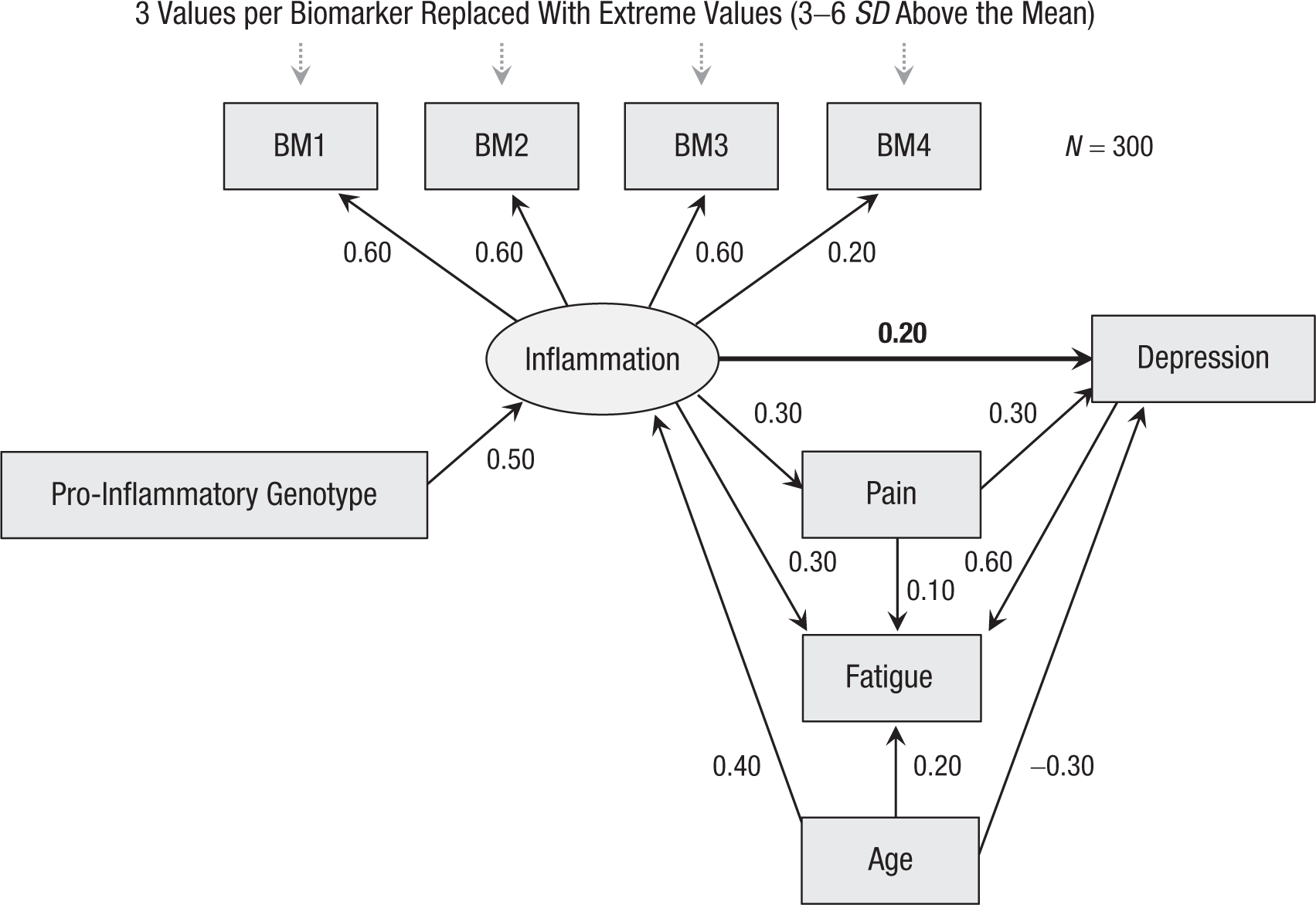
Simulation parameters used to generate the data set for the example (all path coefficients are standardized). The effect of interest is the direct effect of inflammation on depression (thick arrow).

After generating the scores, we replaced three randomly selected cases for each biomarker with extreme values (uniformly sampled between 3 and 6 SD above the mean), to represent laboratory artifacts or atypical physiological states. The final correlation matrix is shown in Table 1. To verify that the particular data set we chose was representative of the universe of possible simulations, we repeated the same analyses on 500 replicate samples (Section S4 of the Supplemental Material). The simulations and analyses were performed in R 3.6 (R Development Core Team, 2019).

Table 1.

Correlation Matrix for the Simulated Data Set

Variable	1	2	3	4	5	6	7	8
1. Age	1.00
2. Genotype	−.03	1.00
3. BM1	.22	.16	1.00
4. BM2	.25	.33	.29	1.00
5. BM3	.24	.30	.31	.31	1.00
6. BM4	.10	−.01	.07	.06	.08	1.00
7. Depression	−.06	.19	.13	.11	.10	−.05	1.00
8. Pain	.14	.17	.13	.15	.16	.00	.41	1.00
9. Fatigue	.24	.23	.26	.30	.24	.07	.65	.42

Note: “BM1” through “BM4” refer to different biomarkers.

Full multiverse-style analyses

In the first set of analyses, we derived a large multiverse of specifications by considering three typical decision nodes: (a) the choice of predictor, (b) the inclusion of alternative covariates, and (c) the cutoff for excluding outliers (by listwise deletion). To mimic the mechanical approach to the multiverse criticized in this article, we did not apply any systematic criteria to the analysis of alternatives, but simply tried to generate as many specifications as possible. We label this the “full” multiverse for the purpose of this example, while recognizing that many other decisions could be considered.

The decision node for the predictor yielded 19 alternatives: each biomarker used individually; biomarkers used individually while controlling for the others (simultaneous entry); and all the possible composites of two, three, and four biomarkers. The decision node for covariates yielded 16 alternatives, corresponding to all the possible combinations of age, pain, fatigue, and genotype. For outliers, we considered four alternatives—analyzing all cases and excluding cases using three common cutoffs: 2.5 SD from the mean, 3.5 SD from the mean, and the first and third quartiles ±1.5 times the interquartile range (Tukey’s fences).

This set of alternatives generates a multiverse of 1,216 effects, which we estimated with linear regression under three types of multiverse-style analyses. First, we plotted and summarized the distribution of p values for the effect of interest (Steegen et al., 2016). Second, we examined the VoE by jointly displaying effect sizes and p values (Patel et al., 2015). Third, we explored the results with a specification curve (Simonsohn et al., 2018, 2020), plotted using the specr package (Version 0.2.1; Masur & Scharkow, 2019).

The distribution of p values and the VoE in the full multiverse are shown in Figure 4. The median p was .194. Just 27% of the effects reached the conventional threshold of α = .05. Effect sizes (β) ranged from −0.16 to 0.25, with a median of 0.01. The VoE plot shows a clear Janus effect (see Patel et al., 2015), as the regression coefficients at the 1st and 99th percentiles of the effect-size distribution have opposite signs (−0.14 and 0.21, respectively). These results could easily be interpreted as indications of poor robustness and replicability. The median effect size across specifications was very close to zero and far from conventional significance thresholds, even though the true effect size in the population was 0.20 (before accounting for measurement validity). Investigators using the mean of the multiverse as a presumably robust estimate would wrongly conclude that the effect of inflammation on depression is about zero.

Fig. 4.

Results of the full multiverse-style analysis of the simulated data set: (a) distribution of p values across the 1,216 specifications and (b) vibration of effects (VoE) plot showing the joint distribution of p values and effect sizes for the same specifications. In VoE plots, the negative logs of p values are plotted. Hence, larger values on the y-axis correspond to smaller p values. The 1st, 50th, and 99th percentiles of the distributions of effect sizes and p values are indicated by the dotted lines.

Figure 5 displays a specification curve for the full multiverse. The significant effects are split between positive and negative. The pattern for alternative predictors reflects the impact of measurement validity, which is lower for individual biomarkers (especially with simultaneous entry) and higher for composites. But the central tendency of effects is similar across predictors. As for covariates, inspection of Figure 5 indicates that combinations that include fatigue tend to yield negative effects, whereas the direction tends to be positive when fatigue is excluded. Regardless of the general direction of effects, every combination produced a fair amount of nonsignificant findings. Alternative cutoffs for outliers do not seem to have had a systematic impact, except that including all cases shifted the distribution toward somewhat more negative effects.

Fig. 5.

Specification curve for the simulated data set (full multiverse of 1,216 specifications). Blue = positive effect sizes significant at α = .05. Red = negative effect sizes significant at α = .05. IQR = interquartile range.

Clearly, the specification curve offers more opportunities to inspect the results for systematic patterns than the summary plots of Figure 4 do. Most investigators would probably recognize that the direction of effects depends strongly on whether fatigue is included as a covariate. Without explicit consideration of measurement validity, the results for alternative predictors may appear to suggest a lack of consistency, or at least marked sensitivity to the precise operationalization of inflammation. Overall, these results could readily be interpreted as a mixture of chance variation and high dependence on the details of the analysis.

Principled multiverse-style analyses

In the second set of analyses, we derived the multiverse in a principled way, by assessing the equivalence of alternatives at each decision node. For predictors, composites are expected to have higher validity than individual biomarkers, and validity is expected to increase as more indicators are included. This is a Type N decision; all else being equal, the preferred option would be a composite of all four biomarkers (BM1 + BM2 + BM3 + BM4). However, there are indications that biomarker BM4 may have low validity, and hence weaken the performance of the composite. For the sake of the example, we assume that these biomarkers are known to be fallible when considered individually. Table 1 shows very small correlations between BM4 and the other biomarkers, and a suspicious near-zero association between BM4 and the pro-inflammatory genotype. Owing to the appreciable sample size of this study, it makes sense to use correlations among biomarkers as indications of their validity.

Without additional information, it is hard to make a confident decision that BM4 should be excluded, but there is a reasonable case for considering the composite BM1 + BM2 + BM3 as an alternative predictor. The question is whether this should be treated as a Type U or Type E decision. Reliability formulas (Section S1 of the Supplemental Material) can be used to explore the consequences of including versus excluding BM4 under a range of assumptions. The worst-case scenario is one in which BM1 through BM3 are moderately valid but BM4 has zero validity; one then expects the validity of the composite with BM4 included to drop by about .06. In the context of this study, we judge this difference to be small enough that the choice between the two composites can be treated as a Type E decision, and the two alternatives can be included in the same multiverse. Note that validity checks on the measures employed in a study can be legitimately performed post hoc, though it is preferable to preregister them whenever potential problems can be anticipated. Also note that we probed the validity of BM4 on the basis of its associations with other indicators and theoretically related variables, not the outcome variable (i.e., depression). This is crucially different from p-hacking the effect of interest (which would be obviously inappropriate), because selecting indicators exclusively on the basis of their intercorrelations cannot systematically inflate their association with the outcome (except for contrived cases in which the outcome is itself correlated with the invalid portion of some indicators).

In addressing the inclusion of covariates, we assume that the researchers are uncertain about which of two causal models of the data is correct: one in which fatigue is a collider (Fig. 2a) and one in which fatigue partly mediates the effect of inflammation on depression (Fig. 2b). (Note that these models predict the same conditional relations among variables, and hence cannot be compared on the basis of their fit to the data.) This is a Type U decision that reflects genuine uncertainty about which alternative is better justified. Accordingly, we constructed two separate multiverses. In the first multiverse (Model 1), fatigue is treated as a collider and excluded from all the specifications; in the second (Model 2), fatigue is treated as a mediator and included in all the specifications. For the remaining covariates, inclusion/exclusion is determined by the causal assumptions that underlie the study (Type N decision): Age is a confounder and should be included, pain is a mediator and also should be included (as the effect of interest is the direct effect), but genotype should be excluded because it may reduce precision (for details, see Section S3 of the Supplemental Material).

Finally, we assume that laboratory artifacts and other atypical biomarker levels are expected in this kind of study. Thus, some form of outlier treatment is preferable over analyzing all cases (Type N decision). In the absence of clear expectations about the distribution of atypical values, the choice among alternative cutoffs is effectively arbitrary. In principle, different cutoffs could result in markedly different sample sizes (and thus lead to power/precision nonequivalence), but this is not the case in the present data set: Sample size under alternative cutoffs ranges from 283 to 289, and the corresponding change in statistical power is negligible. Overall, the choice among alternative cutoffs can be treated as a Type E decision. (For an argument that arbitrary cutoffs are typically unlikely to cause major distortions of research findings, see Fanelli, 2019, p. 34.)

To sum up, a principled evaluation of the decision nodes involved in this analysis yielded a markedly different set of specifications than the first analysis. Instead of a single multiverse with 1,216 specifications, we derived two small multiverses with six specifications each. This reflects the fact that most of the alternatives that make up the full multiverse—in fact, about 99% of them—are not truly arbitrary and should be excluded according to the principles discussed in the previous sections. Some readers may feel that, no matter how well justified, a multiverse of six specifications is too small, and that a credible analysis requires many more models—perhaps a few dozen or hundreds at a minimum. We argue that this intuition should be actively resisted. If a smaller, homogeneous multiverse yields better inferences than a larger one that includes many nonequivalent specifications, it should clearly be preferred.

Figure 6 shows the distribution of p values and the VoE in the two principled multiverses. In the multiverse based on Model 1 (i.e., the true model that generated the data), all six effects were positive and statistically significant at α = .05, with a median p of .012. Effect sizes (β) clustered in a narrow range between 0.14 and 0.16; the median was 0.15. The consistency of effects within this multiverse is reflected in the VoE plot of Figure 6b. In the multiverse based on Model 2 (which incorrectly assumes that fatigue is a mediator), the effects ranged from −0.04 to 0.01, with a median (and mean) of −0.02. These small negative effects failed to meet the threshold for significance; the median p value was .733.

Fig. 6.

Results of the principled multiverse-style analyses of the simulated data set: (a, c) distribution of p values across the six specifications in each of the two multiverses (Model 1 and Model 2) and (b, d) vibration of effects (VoE) plots showing the joint distribution of p values and effect sizes for the same specifications. In VoE plots, the negative logs of p values are plotted. Hence, larger values on the y-axis correspond to smaller p values. The 50th percentiles of the distributions of effect sizes and p values are indicated by the dotted lines.

In sum, analyses of the principled multiverses revealed two homogeneous clusters of effects, indicating that the exact biomarker composite employed as a predictor and the choice of cutoff for outliers do not substantially change the conclusions of the study. What does make a difference is whether fatigue is treated as a collider and excluded as a covariate (Model 1) or treated as a mediator and controlled for in the analysis (Model 2). Making an informed decision between these models would require additional empirical evidence (e.g., experimental or quasi-experimental studies), theoretical developments, or both.

Conclusion

Since becoming aware of it, researchers have increasingly ventured into the multiverse, drawn by its promise of better, more complete, and more transparent treatment of data-analytic decisions. In this article, we have attempted to offer a set of evaluative tools that will help researchers navigate this still largely uncharted territory. To successfully navigate the multiverse, researchers must address a crucial question: What decisions used to specify an analysis are truly arbitrary, such that different options are not expected to yield substantively different answers? Here we have focused on three primary domains of nonequivalence and examined the implications of three kinds of decisions one can make when evaluating alternative specifications.

By no means do we offer an algorithmic solution to the construction of the multiverse. Researchers planning a study face questions about how best to structure and analyze data, and not uncommonly their answers are best guesses (e.g., based on psychometrics or existing theory) rather than rigorously derived solutions; one can expect nothing more of multiverse-style analyses. A key take-home message of this article in that one should also expect nothing less. It makes little sense to include in the multiverse a specification that, a priori, one would have dismissed as inferior to other specifications. Researchers conducting a multiverse-style analysis should clearly and systematically present their rationale for treating alternatives as equivalent.

Type U decisions reflect uncertainty about which of two or more specifications is preferable. We suspect they will not be uncommon. Another take-home message is that such cases call for systematic exploratory multiverse analysis. How do decisions affect effect-size estimates of interest? A posteriori, can one make a convincing case that one set of analyses offers better estimates than others? If not, can one specify the additional data needed to resolve decisions about which estimates are better? In a related vein, Simonsohn et al. (2020) observed, “specification curve analysis will not end debates about what specifications should be run. specification curve analysis will instead facilitate those debates” (p. 1209). However, researchers conducting multiverse-style analyses have not systematically discussed results in this way. In contrast, they have often assumed that when the subspaces of a multiverse yield substantively different answers, the results are simply not robust and hence cannot be trusted. Going forward, multiverse-style methods should not be narrowly thought of as a means to promote transparency in reporting, but rather should be considered an analytic tool that can profitably aid the interpretation of data and inform the development of theoretical models.

Supplemental Material

sj-pdf-1-amp-10.1177_2515245920954925 – Supplemental material for A Traveler’s Guide to the Multiverse: Promises, Pitfalls, and a Framework for the Evaluation of Analytic Decisions

Supplemental material, sj-pdf-1-amp-10.1177_2515245920954925 for A Traveler’s Guide to the Multiverse: Promises, Pitfalls, and a Framework for the Evaluation of Analytic Decisions by Marco Del Giudice and Steven W. Gangestad in Advances in Methods and Practices in Psychological Science