Sage Journals: Discover world-class research

Abstract

Model generalizability describes how well the findings from a sample are applicable to other samples in the population. In this Tutorial, we explain model generalizability through the statistical concept of model overfitting and its outcome (i.e., validity shrinkage in new samples), and we use a Shiny app to simulate and visualize how model generalizability is influenced by three factors: model complexity, sample size, and effect size. We then discuss cross-validation as an approach for evaluating model generalizability and provide guidelines for implementing this approach. To help researchers understand how to apply cross-validation to their own research, we walk through an example, accompanied by step-by-step illustrations in R. This Tutorial is expected to help readers develop the basic knowledge and skills to use cross-validation to evaluate model generalizability in their research and practice.

Keywords

model generalizability cross-validation validity shrinkage open data open materials

A current concern in psychology revolves around the ability to replicate our findings (Open Science Collaboration, 2015). In part, such concerns over replicability reflect an underlying concern with model generalizability (Yarkoni & Westfall, 2017). Model generalizability describes the extent to which statistical models developed in one sample fit other samples from the same population. In general, statistical models tend to not generalize well to a new sample; this is because they capitalize on the unique characteristics of the sample data and tend to produce overly optimistic results (i.e., effect sizes) that overstate the expected effect size in both the population and new samples (e.g., Lord, 1950; Wherry, 1931). Although model generalizability and the key method to assess it—cross-validation—were discussed in the early psychometric literature (e.g., Lord, 1950; Mosier, 1951; Rozeboom, 1981; Wherry, 1931), they have been underemphasized in contemporary psychological training and research (de Rooij et al., 2019). These concepts will become increasingly important for psychological scientists as they strive to conduct replicable research. Thus, our goal in this Tutorial is to re-introduce the concepts of model generalizability and cross-validation to the core training in psychology.

We begin by using a Shiny app to illustrate how statistical models tend to overfit sample data, which leads to poor model generalizability.¹ We demonstrate how model generalizability is affected by model complexity, sample size, and effect size. Next, we briefly describe the concept of cross-validation, review its major steps, and discuss two cross-validation methods researchers may use with their own data (k-fold cross-validation and Monte Carlo cross-validation). We demonstrate the methods by walking through an empirical example using the easy-to-use and powerful R package caret (Kuhn, 2008).

Disclosures

The Shiny app can be accessed at https://qchelseasong.shinyapps.io/CrossValTutorial/, and the data and R code can be accessed at https://osf.io/m62sh/. The Supplemental Material (http://journals.sagepub.com/doi/suppl/10.1177/2515245920947067) provides the code and results for simulations demonstrating model overfit (Appendix A) and cross-validation procedures (Appendix B), as well as an empirical example of cross-validation using the caret R package (Appendix C).

A Demonstration of Model Overfit in a Shiny App

Suppose we want to model the relationship between people’s level of arousal and their performance on a learning task (e.g., how arousal relates to the number of new words memorized). We begin by obtaining a random sample from the population and then use the arousal and task performance measured in this sample to fit a statistical model. For example, we might fit a regression model to the sample data set and obtain the regression coefficients that describe the relationship between arousal and task performance. This sample is called the calibration sample, as the process of estimating the regression coefficients is analogous to “calibrating” the model.

Let us visualize the process using an interactive Shiny app (available at https://qchelseasong.shinyapps.io/CrossValTutorial/). You can interact with the Shiny app using the gray control panel on the left-hand side. To draw a random sample of 50 observations from the population, move the “Calibration Sample Size” slider to 50. Let us assume that, in the population, there is a positive linear relationship between arousal and task performance, and that arousal explains 25% of the variation in task performance (population effect size: ρ² = .25). To specify this in the app, move the “Population Effect Size” slider to .25 and select “Linear” under “Underlying Relationship in the Population.” Then, click on the “Generate Calibration Sample” button to generate a random sample. You will obtain a sample of 50 observations, drawn from a population in which the true relationship between arousal and task performance (ρ²) is .25. A scatterplot with 50 black dots shows up in the Shiny app (see Fig. 1a).² Next, let us fit a regression model to the sample data set and obtain the regression coefficients. When there is only one predictor, the fitted regression model has the following general form:

\hat{y} = b_{0} + b_{1} x + b_{2} x^{2} + . . . + b_{k} x^{k},

where $\hat{y}$ is the predicted value of the outcome (e.g., task performance) when the predictor (e.g., arousal level), $x$ , takes on a particular value. The regression coefficients, b₀, b₁, b₂, . . . , b_k, represent the different forms of the relationship between arousal and task performance. For example, b₁ captures the linear relationship between arousal and task performance, b₂ captures the quadratic relationship between arousal and task performance, and so on.

Fig. 1.

A demonstration of model overfit in the Shiny app. The screenshots show results of the following procedures: (a) generate a calibration sample, (b) fit a simple regression model to the calibration sample, (c) estimate model fit (R² and mean squared error [MSE]) in the calibration sample, and (d) estimate model fit (R² and MSE) in a validation sample.

In this analysis, we are trying to examine both the form and the magnitude of the relationship between arousal and task performance. We start off by estimating a linear regression model: $\hat{y} = b_{0} + b_{1} x$ . In this model, the degree of polynomial is 1 (i.e., $\hat{y} = b_{0} + b_{1} x^{1}$ ): In the Shiny app, use the radio button to set “Degree of Polynomial” to “1.” Then, click on the “Fit the model!” button to fit the regression model (using the calibration sample). The fitted regression line is shown as a black line in the Shiny app (see Fig. 1b). If you select “Show residual errors,” you can see how well the model fits the calibration sample data. This leads us to our first observation:

Observation 1: the model overfits the calibration sample

The regression line in Figure 1b shows the estimated (i.e., expected) task performance at a given level of arousal.³ The black vertical dotted lines represent the residual errors and indicate the extent to which the expected task performance (i.e., points along the solid black line) deviates from the observed task performance (i.e., the black dots). In the regression model, the sum of squared residual errors was minimized to provide the best possible fit to the calibration data.

We use two metrics to examine how well the model fits the data: R² and mean squared error (MSE). R² is typically interpreted as the proportion of the variance in the outcome variable (e.g., task performance) that can be accounted for by the predictors (e.g., arousal level); MSE represents the magnitude of the average squared residual and indicates how much, on average, expected values deviate from observed values. R² (when calculated by squaring correlation coefficients) captures the extent to which expected values exhibit the same rank order as observed values, providing a relative measure of model fit; MSE captures the magnitude of the average squared residual, providing an absolute measure of model fit. As R² and MSE focus on different aspects of model fit, we recommend reporting both metrics.

Now, in the Shiny app, check the “Show R-squared” and “Show MSE” boxes. These values are shown at the top of the scatterplot in Figure 1c: R_Cal² = .45 means that, in the calibration sample, the fitted model (which illustrates the linear relationship between arousal and task performance) accounts for 45% of the variance in task performance; MSE_Cal = 0.48 means that the model’s predictions of task performance will differ from the observed task performance, on average, by a little more than half of a word (i.e., $\sqrt{0.48}$ = 0.69 words) per observation.⁴ The calibration-sample effect size (R_Cal² = 0.45) is almost twice as large as the population effect size (ρ² = .25), which suggests that the model overfitted the calibration data. Overfit occurred because the model captured variation unique to the calibration data that is unrepresentative of the relationship in the population.

Observation 2: the model obtained from the calibration sample tends to not generalize well to new (validation) samples

Thus far, we have used a statistical model to examine the relationship between arousal and task performance in the calibration sample. Often, researchers also want to know whether the findings can be replicated in other samples from the same population. That is, they are interested in whether the model generalizes to a new sample (i.e., the validation sample). In the Shiny app, click on “Test in a new sample!” A validation sample of 1,000 observations will be randomly drawn from the population and used to evaluate the calibrated regression model. The updated result is shown in Figure 1d. Specifically, the app now shows how well the regression model (i.e., the black line) obtained with the calibration sample (i.e., the black dots) predicts task performance from arousal in the validation sample (i.e., the gray dots). That is, the display shows the prediction accuracy of the model (as captured by R_Val² and MSE_Val), which reflects how well the calibrated model is likely to perform in new samples. As shown in Figure 1d, the black line models the relationship between arousal and task performance more poorly in the validation sample than in the calibration sample: Predictions deviate more from the observed values in the validation sample (deviation of 0.88 words, i.e., $\sqrt{M S E_{Val}} = \sqrt{0.78} = 0.88$ ) than in the calibration sample (deviation of 0.69 words).

In addition, as Figure 1d shows, the model explains less variance in the validation sample than in the calibration sample: The model explains 26% of the variance in the validation sample (R_Val² = .26), as compared with 45% of the variance in the calibration sample (R_Val² = .45). This decrease is called validity shrinkage, and it reflects the degree to which the model performs less well in the validation sample. Whereas R_Cal² reflects how well the model fitted the calibration data (including its unique characteristics), R_Val² reflects the accuracy with which the calibrated model predicts the outcome variable of the observations that were not used in fitting the model. Thus, validity shrinkage reflects how well a model generalizes to new samples.

Observation 3: model generalizability is influenced by (a) model complexity, (b) sample size, and (c) effect size

Observation 3a: the model generalizes less well when it is complex

We have modeled the linear relationship between arousal and task performance: $\hat{y} = b_{0} + b_{1} x$ . However, other (nonlinear) forms of the relationship might be plausible. In reality, one usually does not know the true form of the relationship between a predictor and an outcome. To examine if a nonlinear relationship between arousal and task performance is plausible, we could evaluate the fit of more complex models to the data. For example, we could fit a quadratic regression model, $\hat{y} = b_{0} + b_{1} x + b_{2} x^{2}$ ; a cubic regression model, $\hat{y} = b_{0} + b_{1} x + b_{2} x^{2} + b_{3} x^{3}$ ; and so forth. Each additional polynomial term increases the model’s complexity, and by doing so, allows the model to fit the calibration sample more closely.

To see this in the Shiny app, increase “Degree of Polynomial” from 1 to 2 to 3, each time clicking on the “Fit the model!” button to see how well the model fits the calibration sample. As model complexity increases, the regression line fits the data more closely: the cubic regression line fits the calibration sample better than the linear regression line. To examine how well each model performs in the validation sample, keep the “Show R-squared” and “Show MSE” boxes checked and sequentially increase model complexity (i.e., degree of polynomial) from 1 to 2 to 3, each time clicking on the “Test in a new sample!” button to see the validation results. As the complexity of the model increases, R_Val² decreases and MSE_Val increases. In general, as the model becomes more complex, it generalizes less well to other samples in the population.

Observation 3b: the model generalizes less well when the calibration sample size is small

Aside from the model itself, the calibration sample size is also an important factor. Try varying the calibration sample size: In the Shiny app, set the “Calibration Sample Size” to 30, the “Population Effect Size” to .25, and the “Degree of Polynomial” to 1. Then, check the boxes for R² and MSE, and click the “Test in a new sample!” button to see the validation results. Repeat this procedure, increasing the calibration sample size from 30 to 50, then 100, and then 200. In general, as the calibration sample size increases, the difference in R² and MSE between the calibration and validation samples decreases (i.e., validity shrinkage decreases). The model generalizes better when the calibration sample size is large, because large samples tend to be more representative of the population.

Observation 3c: the model generalizes less well when the population effect size is small

Now, we illustrate what happens when the population effect size varies. In the Shiny app, set the “Calibration Sample Size” to 50, the “Population Effect Size” to .01, and the “Degree of Polynomial” to 1. Then, check the boxes for R² and MSE, and click on “Test in a new sample!” Repeat this procedure, each time increasing the population effect size (ρ²) from .01 to .81. In general, as the population effect size increases, the difference in R² between the calibration and validation samples decreases, as does the difference in MSE. That is, as the population effect size increases, the model generalizes better to new samples.

Summary of observations

Together, the observations have shown that a model fitted on one sample (calibration sample) tends to overfit the data and not generalize well to another sample (validation sample; Observations 1 and 2) and that model generalizability decreases as (a) model complexity increases, (b) calibration sample size decreases, and (c) population effect size decreases (Observations 3a, 3b, and 3c).

Because of sampling variation, this general trend might not be observed on every trial. To further illustrate the general trend, we simulated the process in Observations 1, 2, and 3 across multiple trials (trials = 1,000). The R code and results of the simulations are in Appendix A in the Supplemental Material; the simulation results support the observations.

In this example, the relationship in the population was assumed to be linear. However, as suggested by many studies, the relationship between arousal and task performance in the population is most likely to be quadratic (e.g., Hebb, 1955). To see what happens if the form of the relationship in the population is quadratic, in the Shiny app, select the “Quadratic” radio button under “Underlying Relationship in the Population.” Using the “Degree of Polynomial” radio buttons, systematically change the degree of the polynomial of the regression model from 1 to 3 and observe how R² and MSE change. In general, the patterns are consistent with Observations 2, 3a, 3b, and 3c.

Although statistical models commonly overfit the data, it is also possible for them to underfit the data. Model underfit can be caused by sampling variation, as well as model complexity. For example, if the underlying relationship in the population is quadratic, then fitting a linear regression model to the observed data will likely result in model underfit, as the regression model is too simplistic a representation of the underlying relationship in the population. Underfitted models tend to have low model fit (i.e., low R² and high MSE) in both the calibration and the validation samples. Because of this, not only model overfit, but also model underfit can lead to poor model generalizability. Although a thorough discussion of underfitting is beyond the scope of this Tutorial, interested readers can refer to Hastie et al. (2009).

Statistical Models in Psychological Research

Most psychologists are interested in the population-level relationship between the predictor (or predictors) and the outcome. For instance, in our example, we estimated the relationship between arousal and task performance using a regression model. The regression model overfitted the calibration sample, such that the model fit shrank in the validation sample. Further, we also observed that the extent to which the model generalized to other samples in the population depended on three factors: model complexity, sample size, and population effect size.

These factors are particularly relevant to model generalizability in psychological research. At least until very recently, many psychological studies were based on small sample sizes (Shen et al., 2011). For example, in a recent replication attempt examining 28 classic social-psychological studies (Many Labs 2 project; Klein et al., 2018), the median sample size of the original studies was 86.5 (calculated from the raw data: https://osf.io/crz2n/). In addition, because of the complexity in human perception and behavior, the phenomena that psychological studies examine tend to have small effect sizes. For example, in the Many Labs 2 project (Klein et al., 2018), the median Cohen’s d obtained in the replication studies was 0.15. In fact, a summary of the effect sizes reported in social psychology indicated that the median effect size (r) was .25 (Lovakov & Agadullina, 2017; based on k = 98 publications reporting 13,464 associations as Pearson r or Hedges’s g), and a summary of the effect sizes reported in industrial-organizational psychology indicated that the mean effect size (r) was about .22 (e.g., Bosco et al., 2015—based on 147,328 correlations; Paterson et al., 2016—based on 258 meta-analyses). Finally, interaction effects, curvilinear effects, and control variables are often included in the models, increasing model complexity.

In order to minimize model overfit and increase model generalizability, one needs (a) large samples, (b) not-small effect sizes, and (c) models that are not unnecessarily complex. However, this trifecta is rare in psychological research: Increasing the sample size often requires more resources, the size of a given effect is not subject to researchers’ discretion, and the complexity of the model is often guided by theory. Thus, psychological studies are often prone to concerns regarding model generalizability, which suggests there is a need for approaches that could provide additional information on how well statistical models are expected to generalize to new samples. Cross-validation is one such approach.

Cross-Validation: An Approach to Assess Model Generalizability

As demonstrated earlier, one way to evaluate a model’s generalizability is to assess the model on a validation sample. However, obtaining a new sample can be challenging or impractical (e.g., because of limited resources). Cross-validation is an alternative approach that can be used to evaluate model generalizability with the sample one already has (e.g., Hastie et al., 2009).⁵

One can, for example, evenly split the sample data into two sets, then fit (or train) a model in the first set (training set), and evaluate (or test) the generalizability of the model in the second set (test set). If the model fit is similar between the training and test sets, this is initial evidence that the model will generalize well to new samples. However, there are caveats against this procedure: Prediction accuracy is still estimated only once, and the estimate could be influenced by how the training set and test set were partitioned. Thus, most cross-validation approaches repeat this train-then-test cycle in different splits of the data. Put simply, the essence of cross-validation is to generate training and test sets from a single data set so as to repeatedly train and test the model. Although existing cross-validation methods differ in (a) how the data are split and (b) how many repetitions of the train-then-test cycles are conducted, these methods share the same underlying process.

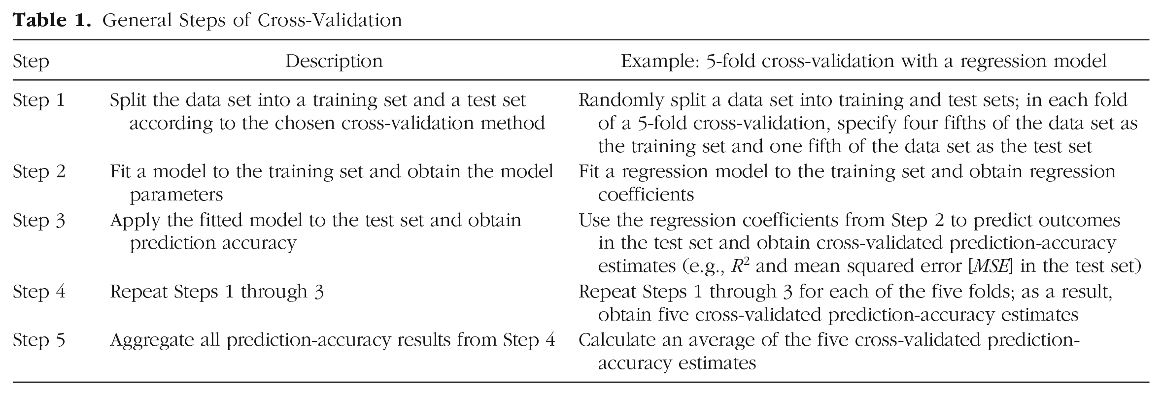
Table 1 summarizes the five steps in cross-validation: (1) obtain training and test sets, (2) fit a model on the training set, (3) apply the fitted model to the test set and obtain prediction accuracy from the test set, (4) repeat Steps 1 through 3, and (5) calculate the average cross-validated prediction accuracy across all the repetitions. The outcome of the procedure—the average cross-validated prediction accuracy—provides an estimate of how well the model will generalize to new samples. Compared with a single train-then-test cycle, repeated train-then-test cycles result in a more stable estimate of cross-validated prediction accuracy, which is less susceptible to random sampling variation.

Table 1.

General Steps of Cross-Validation

Step	Description	Example: 5-fold cross-validation with a regression model
Step 1	Split the data set into a training set and a test set according to the chosen cross-validation method	Randomly split a data set into training and test sets; in each fold of a 5-fold cross-validation, specify four fifths of the data set as the training set and one fifth of the data set as the test set
Step 2	Fit a model to the training set and obtain the model parameters	Fit a regression model to the training set and obtain regression coefficients
Step 3	Apply the fitted model to the test set and obtain prediction accuracy	Use the regression coefficients from Step 2 to predict outcomes in the test set and obtain cross-validated prediction-accuracy estimates (e.g., R² and mean squared error [MSE] in the test set)
Step 4	Repeat Steps 1 through 3	Repeat Steps 1 through 3 for each of the five folds; as a result, obtain five cross-validated prediction-accuracy estimates
Step 5	Aggregate all prediction-accuracy results from Step 4	Calculate an average of the five cross-validated prediction-accuracy estimates

In the following sections, we describe two common cross-validation methods (i.e., k-fold cross-validation [k-fold CV] and Monte Carlo cross-validation [MCCV]), as well as some variations (e.g., repeated k-fold CV, stratified k-fold CV). The k-fold CV and MCCV methods differ in the procedures used to generate the training and test sets; Table 2 provides a comparison of these methods.

Table 2.

Comparison of k-Fold Cross-Validation and Monte Carlo Cross-Validation

Step	Description	Example (N = 200)
Step	Description	k-fold cross-validation(k = 10)	Monte Carlo cross-validation(p = .8, Rep = 100)
Step 0	Prepare the data	Randomly shuffle the observations and divide the data set into 10 (roughly) equal subsets	Decide on p, the proportion of observations randomly sampled as the training set, and Rep, the number of repetitions
Step 1	Split the data set into a training set and a test set	Select the first subset as the test set (200 × .1 = 20 observations) and use the remaining subsets as the training set (180 observations)	Randomly draw 160 observations (without replacement; 200 × .8 = 160) from the data set to form the training set; the remaining 40 observations form the test set
Step 2	Fit a model to the training set and obtain the model parameters	Fit the model to the training set (180 observations)	Fit the model to the training set (160 observations)
Step 3	Apply the fitted model parameters to the test set and obtain the cross-validated prediction accuracy	Test the model from Step 2 in the test set (20 observations)	Test the model from Step 2 in the test set (40 observations)
Step 4	Repeat Steps 1 through 3	Repeat Steps 1 through 3 for each of the 10 folds (10 times)	Repeat Steps 1 through 3 across the specified number of repetitions (100)
Step 5	Calculate an average of all prediction-accuracy results from Step 4	Average the 10 prediction-accuracy results (one for each of the 10 folds) to obtain the overall prediction-accuracy estimate	Average the 100 prediction-accuracy results (one for each of the 100 repetitions) to obtain the overall prediction-accuracy estimate

k-fold cross-validation (Geisser, 1975)

In k-fold CV, the data set is first randomly split into k equal-sized subsets. Then, the train-then-test procedure is repeated k times: Each time, one of the k subsets is used as a test set, and the rest of the k – 1 subsets are used to form the training set. To visualize k-fold CV for a regression model, use the Shiny app with the following inputs (see Fig. 2): “Calibration Sample Size” is 50, “Population Effect Size” is .25, “Underlying Relationship in the Population” is linear, and “Degree of Polynomial” is 3 (i.e., cubic regression). Then, click on the “5-Fold Cross-Validation” button and watch how each step of the 5-fold cross-validation unfolds!

Fig. 2.

An example of a 5-fold cross-validation with a third-order polynomial regression model in the Shiny app.

Figure 2 displays the results of a 5-fold CV. Notice that, in addition to the original scatterplot, there are now five additional plots. Each new plot shows the results from one repetition of the 5-fold CV. For example, in Fold 1, four fifths of the original 50 observations (red dots) were used as the training set, and a cubic regression model (red line) was fitted to these observations. Then, this model was evaluated in the test set (blue dots; i.e., the remaining one fifth of the observations) to obtain an estimate of the cross-validated prediction accuracy (R_CV² and MSE_CV). The train-and-test procedure was carried out five times, each time with one fifth of the data as the test set and the rest as the training set. The way training sets and test sets were partitioned in each fold is also represented visually at the top of the plots, with the red-and-blue bar.

The overall cross-validated prediction accuracy (R_CV.Avg² and MSE_CV.Avg) is calculated by taking the average across the five folds. The results are shown at the top of the Shiny app display. The values in Figure 2 (R_CV.Avg² = .32 and MSE_CV.Avg = 0.66) suggest that if we obtained a new sample from the population, the model fit is likely to be less than .33 (the value obtained in the calibration set) and closer to .32 and MSE is likely to be larger than 0.59 (the value obtained in the calibration set) and closer to 0.66.

Monte Carlo cross-validation (Picard & Cook, 1984)

The MCCV method follows a train-then-test procedure similar to that for k-fold CV. The key distinction is that in MCCV, a predefined proportion of the data set is randomly selected to form the test set in each repetition, and the remaining proportion forms the training set. For example, if the predefined proportion is 20:80, then 20% of the observations will be randomly selected to form the test set, and 80% will form the training set. A model is then fitted to the training set and evaluated on the test set. This random data draw, together with the train-then-test procedure, is repeated a predetermined number of times (e.g., n = 100 repetitions). The overall cross-validated prediction accuracy (R_CV.Avg² and MSE_CV.Avg) is calculated by averaging across the n repetitions.

To examine the MCCV procedure in the Shiny app, simply click the “Monte-Carlo Cross-Validation” button at the bottom of the left-hand bar. As in the k-fold CV demonstration, additional plots are added to the original calibration result, each representing a different repetition. However, unlike in the k-fold CV demonstration, in the red-and-blue bar at the top of each plot (which demonstrates how the data were partitioned into training and testing sets), the red areas (representing the training set) are randomly scattered. This is because, in MCCV, the training set is randomly selected in each repetition, whereas in k-fold CV, the sets are selected sequentially. Appendix B in the Supplemental Material provides the code for a demonstration of how to implement k-fold CV and MCCV in R.

Other cross-validation methods

Over the years, specific extensions to k-fold CV and MCCV have been developed. We briefly mention some of the most common extensions and provide key citations for interested readers who would like to delve more deeply into these specific methods. Leave-one-out cross-validation (LOOCV; Geisser, 1975; Stone, 1974) is a special instance of k-fold CV in which the number of folds is equal to the sample size; this method might be useful when the sample sizes are very small. Repeated k-fold CV (Kim, 2009; Molinaro et al., 2005) extends k-fold CV by conducting multiple repetitions, each of which uses a different k-fold split; this method can provide a more stable estimate of prediction accuracy, as compared with simple k-fold CV.

Both LOOCV and repeated k-fold CV are appropriate for data sets with independent observations. However, many psychological studies use data sets with nested structures that create dependencies in the data; examples include multilevel studies (e.g., students within schools) and within-subjects studies (e.g., repeated measures or longitudinal designs in which the same person provides multiple data points). Extensions of the k-fold CV method have been developed specifically to deal with nested data. For example, if it is important to retain data dependence, group k-fold CV should be used. This method keeps groups intact when the data are partitioned (Kuhn, 2019). If it is important to maintain proportionate representation within a group (e.g., the proportion of women or minorities), then stratified k-fold CV (Kohavi, 1995) is recommended. We note that these extensions of k-fold CV can also be applied to MCCV, in a similar way (for additional information, see Roberts et al., 2017).

Step-By-Step Illustrations in R

In the previous section, we used a Shiny app to help readers visualize the cross-validation procedure and develop an intuition about what happens in each step. In this section, we demonstrate how to conduct cross-validation using the caret R package (Kuhn, 2008). The caret package is a powerful⁶ and easy-to-use toolbox that allows users to conduct cross-validation using just a few simple lines of code. For example, a typical modeling and cross-validation procedure requires only two functions: train() and trainControl(). To illustrate how to conduct cross-validation using caret, we walk through an example based on a publicly available data set, and provide a set of annotated R code that can be easily downloaded and modified for your own use.

Population and calibration sample

Our example data set comes from 71,992 participants who completed the online version of the MACH-IV measure of Machiavellianism (Christie & Geis, 1970). The participants also completed the Ten Item Personality Inventory (TIPI; Gosling et al., 2003), a measure of the Big Five personality traits, and demographic questions. The original data are available from Open-Source Psychometrics Project (2019).⁷

Suppose we were interested in predicting Machiavellianism using Big Five personality, age, and gender. To obtain the population effect size, we treated the 71,992 participants as the population of interest (see Appendix C in the Supplemental Material for details): In the population, the predictor variables explained 28% of the variance in Machiavellianism scores (R_Pop² = .28) and the mean squared distance between the observed Machiavellianism score and fitted score was 0.45 (MSE_Pop = 0.45). A calibration sample (N = 300) was randomly drawn from the population and was then used to fit a regression model. R² in the calibration sample was larger than that in the population (i.e., R_Cal² = .30 vs. R_Pop² = .28), and MSE in the calibration sample was smaller than that in the population (i.e., MSE_Cal = 0.43 vs. MSE_Pop = 0.45). This is because the regression model capitalized on chance variation within the calibration sample. Next, to evaluate model generalizability and obtain more realistic estimates of R² and MSE, we conducted k-fold CV and MCCV.

k-fold cross-validation

A 10-fold CV was implemented on the sample data set using the caret package (see Appendix C in the Supplemental Material). This was done with a few lines of code:



kfold_train_control <-
 trainControl(method = “cv”,
 number = 10)
kfold_cv <- train(mach ~ age +
 as.factor(gender) + O + C + E + A + N,
 data = sample_cal, method = “lm”,
 trControl = kfold_train_control)

The cross-validated R² values are smaller than the calibration-sample R² values (i.e., R_CV.Avg² = .28 vs. R_Cal² = .30), and thus more closely approximate the population R² value of .28. Similarly, the cross-validated MSE values are larger than the calibration-sample MSE values (i.e., MSE_CV = 0.46 vs. MSE_Cal = 0.43). We used nonrepeated k-fold CV here for demonstration purposes only; other more suitable cross-validation methods are available (e.g., repeated k-fold CV, MCCV) and are discussed in the Discussion section.

Monte Carlo cross-validation

Using the caret package, we also implemented MCCV on the sample data set (see Appendix C in the Supplemental Material). The only difference between the R code for MCCV and k-fold CV is a different specification in the trainControl() function:



mc_train_control <- trainControl(method =
 “LGOCV”, p = .8, number = 200)

The Monte Carlo cross-validated R² values are smaller than the calibration-sample R² values (i.e., R_MCCV² = .28 vs. R_Cal² = .30), and more closely approximate the population R² value of .28. Similarly, the MSE values from the MCCV are larger than those obtained in the calibration sample (i.e., MSE_MCCV = 0.46 vs. MSE_Cal = 0.43), and once again closer to the MSE in the population (MSE_Pop = 0.45).

Writing up the results

We could summarize the cross-validation results using the following paragraph:

In order to evaluate the model generalizability of our predicted model, we used the caret package (Version 6.0-86; Kuhn, 2008) in R (Version 3.6.3; R Core Team, 2019) to perform Monte Carlo cross-validation (MCCV; using 200 repetitions and holding out 20% of the sample in each repetition). According to the cross-validation result, when the regression model is generalized to another sample, its prediction accuracy, R², is .28. That is, in a new sample, 28% of the variance in the Machiavellianism scores will likely be accounted for by personality, gender, and age. Additionally, the cross-validated MSE of 0.46 suggests that, on average, the model-predicted Machiavellianism scores will likely deviate from the observed scores in the new sample by 0.68 ( $\sqrt{0.46}$ ) points on a 5-point scale.

Discussion

Choosing among cross-validation methods

As other researchers before us have noted (Arlot & Celisse, 2010; Hastie et al., 2009, Chapter 7; Kuhn & Johnson, 2013), developing clear guidelines for choosing among cross-validation methods is extremely difficult because the choice of specific methods to implement depends on many factors. In practice, these factors include the bias and variance associated with the cross-validated estimates (e.g., R_CV.Avg² and MSE_CV.Avg), as well as the computational cost of a cross-validation method (see Arlot & Celisse, 2010, pp. 68–69; James et al., 2013, pp. 178–184; Kuhn & Johnson, 2013, pp. 69–70). In the context of cross-validation, bias refers to the systematic difference between the population parameter (e.g., ρ²) and the cross-validated estimate (e.g., R_CV.Avg²), and variance refers to the uncertainty (or expected change) in the cross-validated estimates when different data partitions are used (e.g., Kuhn & Johnson, 2013, p. 70). For example, if two implementations of simple 5-fold CV are conducted on a data set, and the cross-validated estimate (e.g., R_CV.Avg²) differs substantially across implementations, this would indicate high variance in the cross-validated estimates. Computational cost (also known as computational complexity) refers to the computation time and the size of computer memory required to implement the cross-validation method. It depends on computer specifications (e.g., processing power, RAM), as well as model specifications (e.g., model complexity, number of partitions or repetitions, and sample size).

Increasing the number of repetitions for a cross-validation method increases the stability of the estimates (i.e., decreases variance), without increasing bias (Molinaro et al., 2005). Thus, repeated k-fold CV and MCCV are generally preferred over simple k-fold CV (Kim, 2009; see also Kuhn & Johnson, 2013, p. 70; Zhang & Yang, 2015). However, in practice, conducting many repetitions is computationally costly (especially when the statistical model is complex), which limits the choice of cross-validation methods.

The effects of bias, variance, and computational cost are further influenced by sample size: When sample size is small, bias and variance are more likely a concern; when sample size is large, computational cost is more likely a concern. Thus, when sample size is small, one could choose repeated k-fold CV or MCCV over simple k-fold CV, as the former yield cross-validated estimates that are less susceptible to high variance (Molinaro et al., 2005). When sample size is large and computational capacity is limited, one could choose simple k-fold CV over repeated k-fold CV and MCCV, as long as one is willing to accept the possibility of less accurate cross-validated estimates (e.g., James et al., 2013).⁸

To sum up, we generally suggest using repeated cross-validation methods (e.g., repeated k-fold CV, MCCV) rather than nonrepeated methods (e.g., simple k-fold CV). However, when computational cost becomes a limitation, and especially when sample size is very large, nonrepeated methods could be considered. In such cases, to examine whether a nonrepeated cross-validation method would yield stable cross-validated estimates in a particular study (which involves a specific sample size and model), we suggest running a few implementations of simple k-fold CV to examine the stability of the cross-validated estimates. If they do not differ much, then a simple k-fold CV is likely sufficient. However, if they vary substantially across implementations (i.e., demonstrate high variance), then the estimates from the simple k-fold CV should be interpreted with caution, and a repeated cross-validation method should be considered instead. When possible, it is advisable to increase computational capacity and use repeated cross-validation methods. Next, we use our Machiavellianism example to illustrate how these guidelines could work in practice.

We conducted a simulation to compare two different cross-validation methods: (a) simple 10-fold CV and (b) repeated 10-fold CV (with 100 repetitions). As with the earlier example, we treated the 71,992 participants in the Machiavellianism data set as the population of interest. Ten different sample-size conditions, with sample sizes varying from 50 to 30,000, were examined. For each sample-size condition, 100 samples (e.g., 100 samples of size 50) were drawn from the population, and for each sample, both simple 10-fold CV and repeated 10-fold CV were implemented. The variance (as represented by the standard deviation) of the R_CV² and MSE_CV and the computational time were recorded for each of the cross-validation procedures and averaged within each sample-size condition; these results are shown in Figure 3.⁹

Fig. 3.

Comparison of the simple and repeated k-fold cross-validation methods. For each sample-size condition, 100 samples were drawn from the population, and for each sample, both simple 10-fold cross-validation (CV) and repeated 10-fold CV were implemented. The following outputs were averaged within each sample-size condition: (a) the variance (i.e., standard deviation) of the cross-validated R², (b) the variance of the cross-validated mean squared error (MSE), and (c) the average time taken to run a cross-validation trial.

In our example, when sample size was smaller than 500, the variance in the cross-validated estimates (i.e., standard deviations of R_CV² and MSE_CV) was much higher for simple k-fold CV than for repeated k-fold CV (see Figs. 3a and b), whereas the absolute difference in computational time between the two methods was only a few seconds (see Fig. 3c). Thus, when sample sizes were smaller than 500, repeated k-fold CV seemed to be the clear method of choice. When sample size was between 500 and 5,000, simple and repeated k-fold CV were similar in the variance of their cross-validated estimates and in computational time. When sample size was larger than 5,000, simple and repeated k-fold CV provided cross-validated estimates with similar variance, but simple k-fold CV was much faster to run than repeated k-fold CV.

In this example, we used simulation to demonstrate how the variance of the cross-validated estimates and computational time differ depending on the cross-validation method and sample size. However, the sample sizes we used are not meant to be universal benchmarks for choosing between simple and repeated k-fold CV: Such choice is highly dependent on specific scenarios (e.g., sample and model). As we described earlier, the variance and computational cost associated with each scenario should be taken into account when choosing among cross-validation methods.

The versatility of cross-validation

In this Tutorial, we have used multiple regression to discuss cross-validation as a method for evaluating model generalizability. Although many indices are already available for assessing model generalizability (e.g., adjusted R²; e.g., Browne, 2000), one advantage of cross-validation is its versatility: It can be adapted for use with many statistical models, and for many different purposes.

Cross-validation does not rely on statistical assumptions (e.g., multivariate normality) and works with almost all types of models. Cross-validation can also be used to select the model (or model parameters) that yield the best prediction accuracy. This practice is known as hyperparameter tuning (see Bergstra et al., 2011; Kuhn & Johnson, 2013, p. 66; Pedregosa et al., 2011). Hyperparameter tuning is part of the standard procedure of many machine-learning models: It can help optimize the degree of polynomial terms used in a linear regression model, the maximum depth allowed for in a decision-tree model, and the number of neurons used in a neural-network model, among others. Hyperparameter tuning, or model selection via cross-validation, can be achieved with various statistical tools, such as the caret package, as well as the cv.glmnet() function in the glmnet package (Friedman et al., 2010) in R.

Cross-validation is particularly useful—and especially important—in high-dimensional situations with many predictors. First, models fitted on high-dimensional data tend to overfit the data, and thus we recommend using cross-validation to evaluate model generalizability in high-dimensional situations (James et al., 2013; for instructions on how to conduct cross-validation in high-dimensional situations, see Hastie et al., 2009). Second, cross-validation can also be used to minimize model overfit in high-dimensional data. For example, regularization techniques, a promising approach to minimize model overfit, often rely on cross-validation (specifically, hyperparameter tuning) to find the best parameters that minimize model overfit.¹⁰ In short, cross-validation is a versatile method that helps researchers evaluate model generalizability, conduct model selection, and reduce model overfit in high-dimensional situations.

Summary

An ongoing concern in the field of psychology revolves around the difficulty of reproducing results obtained in an original study in subsequent replication efforts (e.g., Open Science Collaboration, 2015). Even when the presence or absence of an effect is reproduced in a subsequent study, the effect is often smaller than what was initially reported (e.g., Klein et al., 2018). This is actually less unexpected than it would seem: Because of model overfit, the effect size obtained in a given sample tends to overstate the effect size in a population (e.g., Wherry, 1931) or in a new sample (Lord, 1950).¹¹ In this Tutorial, our goal has been to demonstrate cross-validation as a method for obtaining more accurate estimates of the magnitude of effect sizes in new samples.

In particular, we discussed model generalizability by explaining and demonstrating model overfit and how it results in validity shrinkage in new samples. Next, we reviewed the basic steps of cross-validation (see Table 1) and discussed two common cross-validation methods (i.e., k-fold CV and MCCV; see Table 2). Finally, we demonstrated the methods using an empirical data set and provided a step-by-step illustration of how to implement the cross-validation methods using the caret R package (see Appendix C in the Supplemental Material).

Cross-validation is not a substitute for replication efforts; in fact, they are conceptually distinct and represent complementary approaches for fostering robust and reliable science (Bollen et al., 2015). Cross-validation is mainly focused on whether a particular fitted model performs well in a new sample; replicability efforts often focus on whether researchers can observe effects that are similar to those found in the original study. Although replication efforts are crucial, not all (in fact, a very small number of) research teams have the resources to conduct large-scale replication studies. Cross-validation could contribute important information regarding generalizability that is easily obtained, thus providing an invaluable tool to advance reliable and robust science.

Supplemental Material

sj-docx-1-amp-10.1177_2515245920947067 – Supplemental material for Making Sense of Model Generalizability: A Tutorial on Cross-Validation in R and Shiny

Supplemental material, sj-docx-1-amp-10.1177_2515245920947067 for Making Sense of Model Generalizability: A Tutorial on Cross-Validation in R and Shiny by Q. Chelsea Song, Chen Tang and Serena Wee in Advances in Methods and Practices in Psychological Science

Footnotes

Transparency

Action Editor: Frederick L. Oswald

Editor: Daniel J. Simons

Author Contributions

Q. C. Song, C. Tang, and S. Wee jointly generated the initial idea and outline for the Tutorial. Q. C. Song developed the Shiny app, and C. Tang and S. Wee provided feedback on it. C. Tang wrote and annotated the R codes, and Q. C. Song and S. Wee edited the annotations and code. C. Tang initiated an outline draft of the introduction and the section titled A Demonstration of Model Overfit in a Shiny App, and Q. C. Song wrote a complete first draft of those sections. S. Wee wrote a complete first draft of the section titled Step-by-Step Illustrations in R, and C. Tang provided additional details. Q. C. Song created Figure 1, Figure 2, and Table 1. C. Tang created Table 2 and . All the authors critically edited the full manuscript and approved the final submitted version of the manuscript.

ORCID iDs

Q. Chelsea Song

Serena Wee

Supplemental Material

Additional supporting information can be found at

Notes

References

Arlot

Celisse

(2010). A survey of cross-validation procedures for model selection. Statistics Surveys, 4, 40–79.

Bergstra

Bardenet

Bengio

Kégl

(2011). Algorithms for hyper-parameter optimization. In Shawe-Taylor

Zemel

Bartlett

Pereira

Weinberger

K. Q.

(Eds.), Advances in neural information processing systems 24: 25th annual conference on neural information processing systems 2011 (pp. 2546–2554). Neural Information Processing Systems Foundation.

Bollen

Cacioppo

J. T.

Kaplan

R. M.

Krosnick

J. A.

Olds

J. L.

Dean

(2015). Social, behavioral, and economic sciences perspectives on robust and reliable science: Report of the Subcommittee on Replicability in Science Advisory Committee to the National Science Foundation Directorate for Social, Behavioral, and Economic Sciences. National Science Foundation. https://www.nsf.gov/sbe/AC_Materials/SBE_Robust_and_Reliable_Research_Report.pdf

Bosco

F. A.

Aguinis

Singh

Field

J. G.

Pierce

C. A.

(2015). Correlational effect size benchmarks. Journal of Applied Psychology, 100(2), 431–449.

Browne

M. W.

(2000). Cross-validation methods. Journal of Mathematical Psychology, 44(1), 108–132.

Christie

Geis

(1970). Studies in Machiavellianism. Academic Press.

de Rooij

Pratiwi

B. C.

Fokkema

Dusseldorp

Kelderman

(2019). The early roots of statistical learning in the psychometric literature: A review and two new results. arXiv. https://arxiv.org/abs/1911.11463

Friedman

Hastie

Tibshirani

(2010). Regularization paths for generalized linear models via coordinate descent. Journal of Statistical Software, 33(1). https://doi.org/10.18637/jss.v033.i01

Geisser

(1975). The predictive sample reuse method with applications. Journal of the American Statistical Association, 70(350), 320–328.

10.

Gosling

S. D.

Rentfrow

P. J.

Swann

W. B.

Jr. (2003). A very brief measure of the Big-Five personality domains. Journal of Research in Personality, 37(6), 504–528.

11.

Hastie

Tibshirani

Friedman

(2009). The elements of statistical learning: Data mining, inference, and prediction (Springer Series in Statistics). Springer.

12.

Hebb

D. O.

(1955). Drives and the C. N. S. (conceptual nervous system). Psychological Review, 62(4), 243–254.

13.

James

Witten

Hastie

Tibshirani

(2013). An introduction to statistical learning. Springer.

14.

Kim

J.-H.

(2009). Estimating classification error rate: Repeated cross-validation, repeated hold-out and bootstrap. Computational Statistics and Data Analysis, 53(11), 3735–3745.

15.

Klein

R. A.

Vianello

Hasselman

Adams

B. G.

Adams

R. B.

Jr. Alper

Aveyard

Axt

J. R.

Babalola

M. T.

Bahník

Š.

Batra

Berkics

Bernstein

M. J.

Berry

D. R.

Bialobrzeska

Binan

E. D.

Bocian

Brandt

M. J.

Busching

. . . Nosek

B. A.

(2018). Many Labs 2: Investigating variation in replicability across samples and settings. Advances in Methods and Practices in Psychological Science, 1(4), 443–490.

16.

Kohavi

(1995). A study of cross-validation and bootstrap for accuracy estimation and model selection. In Proceedings of the Fourteenth International Joint Conference on Artificial Intelligence (Vol. II, pp. 1137–1143). International Joint Conferences on Artificial Intelligence Organization.

17.

Kuhn

(2008). Building predictive models in R using the caret package. Journal of Statistical Software, 28(5). https://doi.org/10.18637/jss.v028.i05

18.

Kuhn

(2019). 4.4: Simple splitting with important groups. In The caret package. http://topepo.github.io/caret/data-splitting.html#simple-splitting-with-important-groups

19.

Kuhn

Johnson

(2013). Applied predictive modeling. Springer.

20.

Lord

F. M.

(1950). Efficiency of prediction when a regression equation from one sample is used in a new sample. ETS Research Bulletin Series, 1950(2). https://doi.org/10.1002/j.2333-8504.1950.tb00478.x

21.

Lovakov

Agadullina

E. R.

(2017). Empirically derived guidelines for interpreting effect size in social psychology. https://psyarxiv.com/2epc4/download/?format=pdf

22.

Molinaro

A. M.

Simon

Pfeiffer

R. M.

(2005). Prediction error estimation: A comparison of resampling methods. Bioinformatics, 21(15), 3301–3307.

23.

Mosier

C. I.

(1951). I. Problems and designs of cross-validation 1. Educational and Psychological Measurement, 11(1), 5–11.

24.

Muirhead

R. J.

(1985). Estimating a particular function of the multiple correlation coefficient. Journal of the American Statistical Association, 80(392), 923–925. https://doi.org/10.1080/01621459.1985.10478204

25.

Open Science Collaboration. (2015). Estimating the reproducibility of psychological science. Science, 349(6251), Article aac4716. https://doi.org/10.1126/science.aac471

26.

Open-Source Psychometrics Project. (2019). Raw data from online personality tests [Data set]. Author. https://openpsychometrics.org/_rawdata/

27.

Paterson

T. A.

Harms

P. D.

Steel

Credé

(2016). An assessment of the magnitude of effect sizes: Evidence from 30 years of meta-analysis in management. Journal of Leadership & Organizational Studies, 23(1), 66–81.

28.

Pedregosa

Varoquaux

Gramfort

Michel

Thirion

Grisel

Blondel

Prettenhofer

Weiss

Dubourg

Vanderplas

Passos

Cournapeau

Brucher

Perrot

Duchesnay

. (2011). Scikit-learn: Machine learning in Python. Journal of Machine Learning Research, 12(85), 2825–2830. https://www.jmlr.org/papers/volume12/pedregosa11a/pedregosa11a.pdf

29.

Picard

R. R.

Cook

R. D.

(1984). Cross-validation of regression models. Journal of the American Statistical Association, 79(387), 575–583.

30.

R Core Team. (2019). R: A language and environment for statistical computing (Version 3.6.3) [Computer software]. R Foundation for Statistical Computing. https://www.R-project.org/

31.

Roberts

D. R.

Bahn

Ciuti

Boyce

M. S.

Elith

Guillera-Arroita

Hauenstein

Lahoz-Monfort

J. J.

Schröder

Thuiller

Warton

D. I.

Wintle

B. A.

Hartig

Dormann

C. F.

(2017). Cross-validation strategies for data with temporal, spatial, hierarchical, or phylogenetic structure. Ecography, 40(8), 913–929.

32.

Rozeboom

W. W.

(1981). The cross-validational accuracy of sample regressions. Journal of Educational Statistics, 6(2), 179–198.

33.

Shen

Kiger

T. B.

Davies

S. E.

Rasch

R. L.

Simon

K. M.

Ones

D. S.

(2011). Samples in applied psychology: Over a decade of research in review. Journal of Applied Psychology, 96(5), 1055–1064.

34.

Stone

(1974). Cross-validatory choice and assessment of statistical predictions. Journal of the Royal Statistical Society: Series B (Methodological), 36(2), 111–133.

35.

Wherry

R. J.

(1931). A new formula for predicting the shrinkage of the coefficient of multiple correlation. Annals of Mathematical Statistics, 2(4), 440–457.

36.

Yarkoni

Westfall

(2017). Choosing prediction over explanation in psychology: Lessons from machine learning. Perspectives on Psychological Science, 12(6), 1100–1122.

37.

Zhang

Yang

(2015). Cross-validation for selecting a model selection procedure. Journal of Econometrics, 187(1), 95–112.

Supplementary Material

Please find the following supplemental material available below.

For Open Access articles published under a Creative Commons License, all supplemental material carries the same license as the article it is associated with.

For non-Open Access articles published, all supplemental material carries a non-exclusive license, and permission requests for re-use of supplemental material or any part of supplemental material shall be sent directly to the copyright owner as specified in the copyright notice associated with the article.

0.00 MB

0.06 MB