
Abstract
Sometimes interesting statistical findings are produced by a small number of “lucky” data points within the tested sample. To address this issue, researchers and reviewers are encouraged to investigate outliers and influential data points. Here, we present StatBreak, an easy-to-apply method, based on a genetic algorithm, that identifies the observations that most strongly contributed to a finding (e.g., effect size, model fit, p value, Bayes factor). Within a given sample, StatBreak searches for the largest subsample in which a previously observed pattern is not present or is reduced below a specifiable threshold. Thus, it answers the following question: “Which (and how few) ‘lucky’ cases would need to be excluded from the sample for the data-based conclusion to change?” StatBreak consists of a simple R function and flags the luckiest data points for any form of statistical analysis. Here, we demonstrate the effectiveness of the method with simulated and real data across a range of study designs and analyses. Additionally, we describe StatBreak’s R function and explain how researchers and reviewers can apply the method to the data they are working with.
Assessing the replicability of statistical findings is an important concern in the psychological sciences (Freese & Peterson, 2017; Open Science Collaboration, 2015). One reason for replication failures is that original results may depend on the presence of “lucky” observations; that is, the findings may rest on a small number of unique data points (Osborne & Overbay, 2004). Yet individual data points are rarely analyzed, possibly because of the large number of alternative (and perhaps arbitrary) methods, metrics, and rules of thumb for case exclusions (Chawla & Gionis, 2013; Cousineau & Chartier, 2010; Langford & Lewis, 1998; Leys, Klein, Dominicy, & Ley, 2018; Leys, Ley, Klein, Bernard, & Licata, 2013; Sawant, Billor, & Shin, 2012). Additionally, recent debates about questionable research practices may lead researchers to be reticent about case analyses and exclusions (Bakker & Wicherts, 2014a; Wicherts et al., 2016). As a result, researchers frequently avoid such diagnostic analyses, thereby potentially endangering the reliability and validity of their conclusions (cf. Leys et al., 2018; Osborne, Christiansen, & Gunter, 2001).
In this article, we introduce the StatBreak algorithm (implemented as an R function; https://osf.io/fmnxp/), which highlights the observations most strongly contributing to an interesting finding. More precisely, StatBreak answers the following question: Which (and how few) cases would need to be excluded from a given sample to yield a different statistical conclusion? The algorithm searches for data points that most strongly influence a conclusion-relevant statistic (e.g., p value, Bayesian posterior, or number of components in a principal components analysis) in the hypothesized direction. Investigating which data points contributed most strongly to an interesting finding implies a conservative stance by the researcher. However, StatBreak does not answer the question of whether the luckiest data points should be excluded, and it is therefore complementary to the methods of outlier exclusion that are based on preregistered metrics and cutoffs (Leys et al., 2018).
Facilitating Conservative Outlier Analyses
Individual case analyses are burdensome and increase researcher degrees of freedom, as there are many potential reasons to include or exclude observations from the focal analyses. In regression models, for instance, individual outliers can be identified on the basis of model residuals, extreme predictor values (i.e., leverage points), or the extent to which data points shift predictions or model coefficients (e.g., difference in fits, or DFFITS: Welsch & Kuh, 1977; Cook’s distance: Cook, 1977). Each of these criteria can be assessed with multiple metrics, and for each metric there are multiple cutoffs for case exclusions. Additionally, there are multiple approaches to implementing individual procedures; for instance, procedures may be executed once or stepwise by reestimating model residuals after each case exclusion. Thus, although case analyses can facilitate a better understanding of the data, they are difficult to navigate and can be exploited toward preferred findings by choosing the metrics and cutoffs that give the desired results. It quickly becomes apparent why outlier exclusions are often judged as suspicious by readers, or not considered by researchers (Bakker & Wicherts, 2014a; Wicherts et al., 2016).
StatBreak is aimed at responding to these concerns by facilitating conservative and simple case analyses, and it can produce interpretable results for any form of statistical analysis. Essentially, it does so by identifying the smallest sample subset that needs to be excluded for a conclusion-relevant pattern (e.g., large effect or small p value) to disappear. The nature and size of this subset informs users of the robustness of the original conclusion. StatBreak delivers readable outputs across different types of analyses (indicating that the initial statistical conclusion changes when certain observations are excluded) and can thereby serve as a conservative reference point for cutoff-based outlier detection (observations flagged for exclusion are suspicious).
Disclosures
All data and materials for this article, including the StatBreak R package, can be obtained on the Open Science Framework (OSF), at https://osf.io/fmnxp/.
Identifying Influential Subsamples
Finding a data subset with a desired set of characteristics presents a computational challenge, as there are many possible subsets that could be investigated. For instance, if a researcher’s original sample consists of 200 observations, then there are 2200 – 1 possible subsets of the sample that would need to be examined. Genetic algorithms solve this problem by quickly approximating an optimal solution for such expensive computational tasks (see the materials on OSF for a comparison of the convergence reliability and efficiency of genetic algorithms and other search algorithms, such as the Artificial Bee Colony algorithm). Here, we describe how genetic algorithms can be applied to examine the robustness of conclusions drawn from an observed statistic.
In StatBreak, a genetic algorithm (for an introduction, see Chatterjee, Laudato, & Lynch, 1996) is used to find the largest subset of observations in which a statistical result is not observed, or is altered beyond a conclusion-relevant threshold. This genetic algorithm is specified as follows: First, randomly sized subsamples of the original data set are drawn. These subsamples differ in which observations are included and excluded (e.g., Subsample A includes Observations 1, 2, and 5, whereas Subsample B includes Observations 2 and 4). Each subsample is assigned a fitness score, defined as a function of the generated sample statistic and the size of the subsample: the less interesting the sample statistic and the fewer cases excluded from the original sample, the higher the fitness of the subsample. For example, a subsample that excludes many observations and has a purportedly interesting target statistic (e.g., a high correlation) would receive a low fitness score. On the other hand, a subsample that excludes a small number of observations and has a relatively uninteresting target statistic (e.g., a correlation of zero) would receive a high fitness score.
This definition of fitness is somewhat counterintuitive, as researchers would usually characterize noninteresting findings as low in fitness. However, StatBreak does not try to find interesting patterns; rather, it investigates whether the sample would have produced a different conclusion had it not been for a few data points. The fittest subsamples (having the largest numbers of observations and the least interesting findings) are retained and form part of a next generation of subsamples (i.e., they survive). The next generation of subsamples is created by merging characteristics of two parent subsamples (e.g., exclude Observation 1 as Parent A did, include Observation 2 as Parent B did, etc.). The higher the fitness of a current subsample, the more likely it is to be selected as a parent for the next generation.
Additionally, some random mutations are introduced into the process; that is, in some subsamples of the next generation, the inclusion or exclusion of some cases is randomly flipped. After a number of generations, the algorithm converges to find the fittest generation members, which are the subsamples with the largest amount of observations that generate effects smaller than the minimum effect of interest (e.g., rs < .3, Bayes factors < 3, p values higher than the α level) or other findings resulting in conclusions different from the initial one. In short, StatBreak optimizes a statistic by creating different subsamples of data, quantifying how well each subsample works (fitness), and then exploring in the direction that gives the best (fittest) results. An illustration of this process is presented in Figure 1.
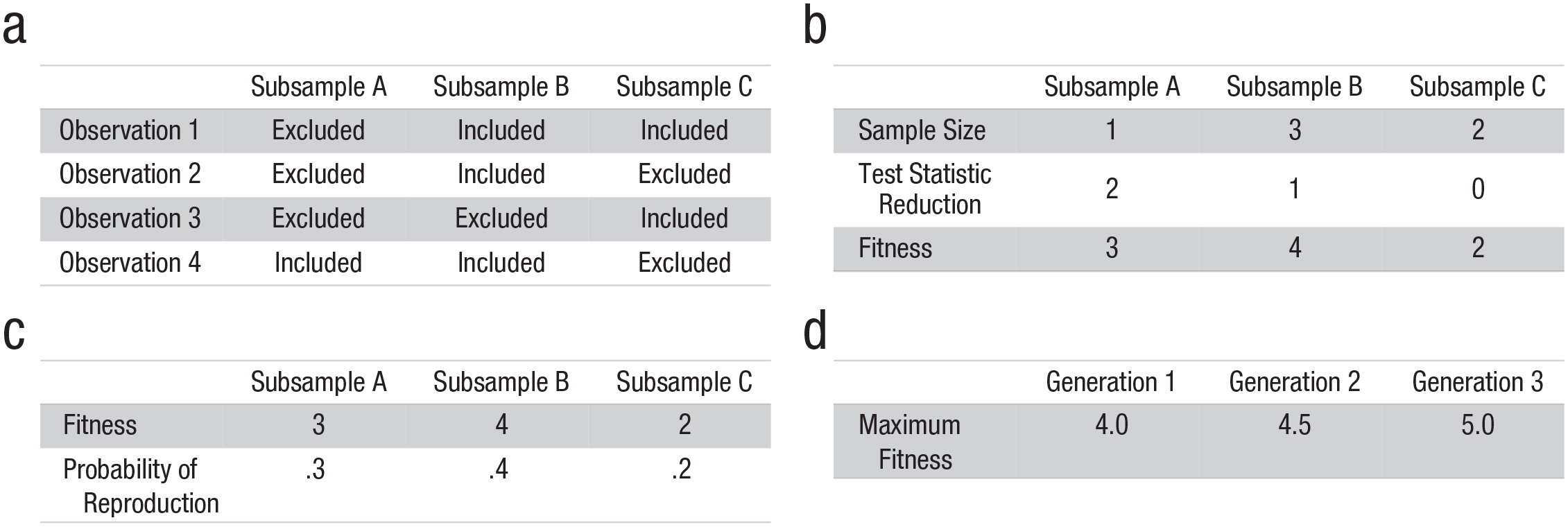
Four-step visualization of the genetic algorithm underlying StatBreak. First (a), an initial population of subsamples is randomly generated. Each subsample includes a random set of observations from the sample. Second (b), the fitness of each subsample is assessed. Subsamples that exclude fewer observations and have less interesting target statistics (e.g., lower r, higher p) receive higher fitness scores. Third (c), subsamples with higher fitness levels are more likely to be included and create similar offspring in the next generation, which increases the overall fitness of future generations. Finally (d), the process is iterated until an optimal subsample is found. This is the largest subsample with the least interesting result (i.e., it excludes the luckiest cases).
By examining which (and how few) cases were dropped from the original sample to arrive at the fittest generation member, users can assess the robustness of the original conclusion. For example, this process might reveal that a significant test statistic can be attenuated to nonsignificance by excluding only one specific case. In this article, we explain how to set up the StatBreak algorithm (e.g., how to determine the population size) and subsequently demonstrate how to apply it with simulated and real data. We also provide some guidance on how to interpret and report results delivered by the algorithm, which can be accessed through an R package.
StatBreak’s Parameters
When running a genetic algorithm to assess the robustness of an initial conclusion, one needs to provide the algorithm with the original sample of observations as well as the statistic of interest (e.g., Cohen’s d, Bayes factor, or local coefficient in a structural equation model). Additionally, the following four parameters form part of the StatBreak algorithm: (a) the number of subsamples to generate in each generation, (b) the function that will be used to compute the fitness of each subsample, (c) how a new generation of subsamples will be formed, and (d) the probability of random mutations.
We chose conservative defaults for these parameters in the R package, though these defaults can be tuned if convergence fails, which should not be the case for most analyses in psychological science. Even for a very challenging search situation (finding 5 outliers in 10,000 observations), StatBreak found the exact subset in 100 out of 100 trials using our default parameters (see the materials on OSF).
Generation size
Having more generation members (i.e., subsamples) per generation ensures a more comprehensive search for an optimal solution, but also requires more computational resources. We advise researchers to use StatBreak’s default of 1,000 generation members and increase this number if no convergence is achieved.
The fitness function
This function quantifies the fitness of individual generation members (i.e., subsamples). There are two objectives that need to be integrated into the function. The first is to retain as many observations as possible (i.e., to discard as few as possible). The second is for the target statistic to lie below or above an (explicitly justified) conclusion-relevant cutoff (e.g., p > α or effect size < the smallest effect size of interest). An example for such a fitness function is this: 1
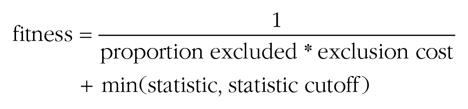
From the formula, it follows that fitness increases with a lower proportion of exclusions and a higher statistic (e.g., a higher p value), but only if the prespecified cutoff (e.g., α) is not yet achieved. Notice that some statistics (e.g., effect sizes) need to be decreased through the algorithm. In these cases, the fitness function is automatically changed to

It might seem desirable for the fitness function to be hierarchical, that is, to first prioritize reaching the goal statistic (e.g., p > α) and to treat optimizing the number of exclusions as a secondary consideration. In other words, the algorithm might consider exclusions only after the goal statistic is reached, so as to allow for conclusions such as “For the effect to ‘disappear,’ these two observations need to be excluded.” This would require the first term in the function (1/(proportion excluded * exclusion cost)) to be dominated by the second term (max(statistic, statistic cutoff) or min(statistic, statistic cutoff)); that is, changes to the second term should have larger effects on the overall fitness score. Unfortunately, this dominance is not guaranteed, as different statistics have very different scales. However, we conducted experiments (which we report later) and found that setting the exclusion cost to 0.01 serves to generate optimal solutions for a wide range of sample sizes and various statistics commonly used in psychological research.
Keeping track of the current fittest member across generations shows whether the default fitness function is working. More precisely, the continuous output of the algorithm, which includes the current leader’s subset size and sample statistic, should show incremental growth of the leader’s subset size conditional on a goal statistic being reached. If this growth is not observed, the fitness function can be tuned by adjusting the exclusion cost. However, in our experiments that was never necessary. Figure 2 illustrates a fitness mapping across values of a sample statistic and the percentage of deleted cases.
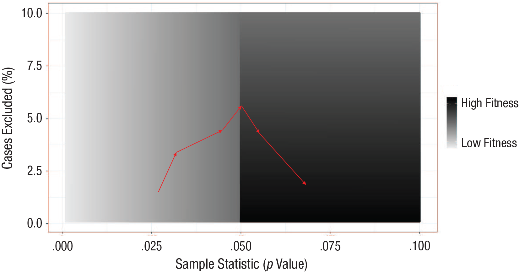
An example distribution of fitness scores generated by StatBreak. The chosen goal cutoff lies at p = .05 (higher values are less interesting), and the purpose of the algorithm is to reach this goal while excluding as few cases as possible from the original sample. The five red triangles show how the fittest subset might improve over the first five generations. Notice that the algorithm first improves fitness by focusing on optimizing the sample statistic (p value; x-axis); then, once the minimum desired p value is reached, the algorithm also begins to improve fitness by reducing the percentage of excluded cases (y-axis).
Reproduction procedure (fixed; not part of the adjustable arguments in StatBreak’s R function)
In our implementations of the algorithm, the generation members with the top 10% of fitness scores are directly copied into the next generation without changes. This ensures that good solutions are not forgotten. The other 90% of the new generation is generated by repeatedly picking two parent subsets from the prior generation, mixing their genetic information, and introducing some random mutations (see Fig. 3). The probability of being picked as a parent subset is proportional to a subset’s relative fitness.
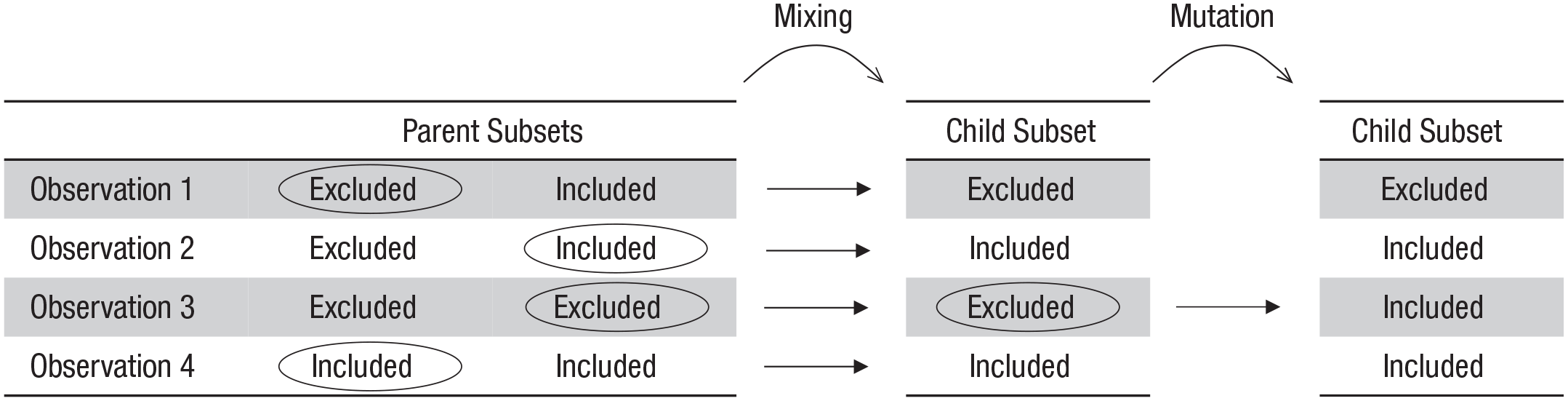
StatBreak’s process of generating a new subset from two subsets of the previous generation. Each parent subset has a set of binary characteristics (i.e., whether each observation is excluded or included). For each characteristic, the parent whose value will be passed on to the new subset is randomly chosen (circled). Subsequently, values of some of the descendants’ characteristics are flipped during mutation (circled).
Random mutations
A higher chance for random mutations leads to a more comprehensive but slower search for an optimal solution. We obtained good results with mutation probabilities between .02 and .05. As did generation size, this parameter affected how quickly the optimal solution was found (usually in less than a minute for most data-set sizes and statistics in psychological research), but never whether the solution was found at all.
Default settings
For all application of StatBreak reported in this article, we used the default settings. Thus, our results highlight that there is rarely a reason to deviate from the default parameters. All the computations were performed on a laptop with 8 GB of RAM and an Intel core i5 processor.
Simulations
The StatBreak algorithm allows researchers and reviewers to investigate the robustness of conclusions, by indicating which (and how few) cases would need to be excluded to yield a different statistical conclusion in reference to a justified threshold. To test whether analyses conducted with StatBreak ascribe greater robustness to studies with larger sample sizes and effects, we conducted a comprehensive simulation study. We simulated data sets with two variables (M = 0, SD = 1); sample sizes ranged from 100 to 1,000 observations, and population correlations ranged from .2 to .8. We then ran StatBreak on the sample correlations, indicating that we wanted to know which and how many observations would need to be deleted to obtain a nonsignificant finding (p > .05). In other words, we used the p value as StatBreak’s target statistic and .05 as the conclusion-relevant cutoff. We repeated these simulations for population-level correlations of 0 under random inclusion of outliers (i.e., outliers took on random values until they shifted the p value to under .05). The results of this simulation study are depicted in Figure 4.
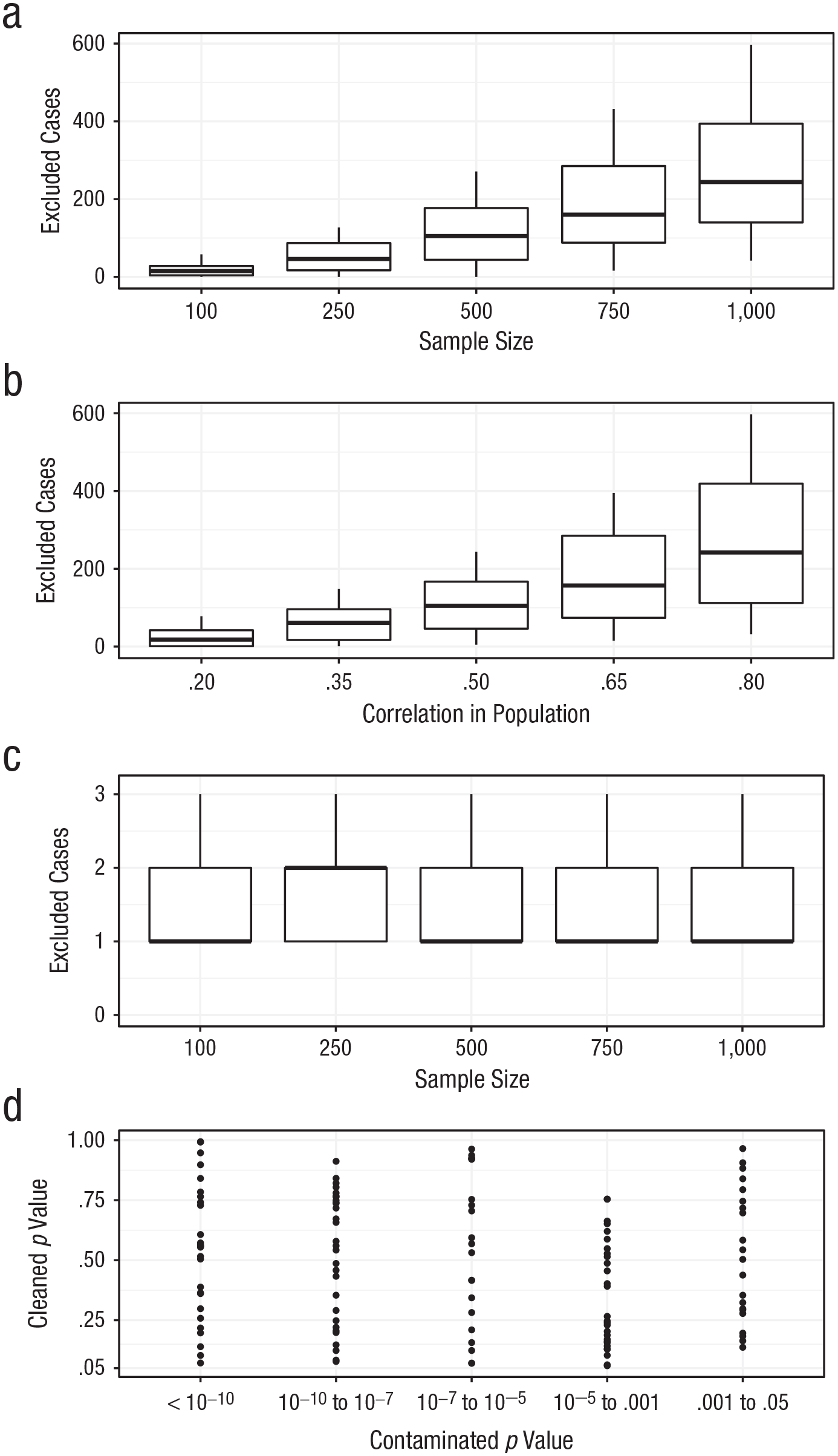
Results from applying StatBreak to the simulated data. The graphs in (a) and (b) show results for data sets with a nonzero population-level correlation. These graphs show the number of observations that would need to be excluded to change a statistically significant (p < .05) finding into a nonsignificant one (p > .05) as a function of (a) sample size and (b) effect size. The graphs in (c) and (d) show results for data sets with a zero population-level correlation. As does the graph in (a), the graph in (c) shows the number of observations that would need to be excluded to change a statistically significant finding into a nonsignificant one, but in this case the numbers are much smaller and do not covary with sample size, because a small set of outliers caused the significant finding and removing them is sufficient to change the result. The graph in (d) shows how the initial, contaminated p values change if the flagged cases (in this case, these are outliers) are excluded. In (a), (b), and (c), each box indicates the middle 50% of values, the horizontal line inside the box indicates the median, and the vertical lines represent the range from lowest to highest number of excluded cases.
The results of our first simulations demonstrate that the proportion of required case deletions is positively related to the original sample size and the size of the effect in the population (Figs. 4a and 4b). For example, the effect in a study with 100 observations and a population-level correlation of .20 can be attenuated to nonsignificance (p > .05) by removing an average of 1.12% of the sample (i.e., a single observation). This is not surprising, given that the statistical power to obtain a significant result in this scenario (1 – β) is only .65 in the first place. That is to say, StatBreak’s indication that a finding is not robust might sometimes be due to a lack of power rather than a single influential data point. A closer inspection of the data point in question can clarify why the conclusion threshold was crossed, and if the data point is not suspicious, removing it would bias the alpha level downward. On the other hand, the effect in a study with 250 observations and a population correlation of .35 can be attenuated to nonsignificance only by removing on average 8.2% of the sample (or a total of 21 observations). This increase in the stability of results with growing sample size has been described comprehensively in simulation studies by Schönbrodt and Perugini (2013). The fact that StatBreak flags these observations does not mean that they should be removed. StatBreak merely highlights them as the strongest contributors to the significant finding. When the number of flagged cases is low (e.g., Fig. 4c) and removing them leads to a large change in the statistic of interest (see Fig. 4d), then it is likely that the flagged cases are outliers. However, a qualitative review of the observations in question is still required.
In actual analyses, outliers affecting the p value of a bivariate correlation are relatively likely to be noticed because they are visibly removed from the point cloud in a scatterplot. However, outliers are less likely to be noticed (and discussed) when more than two variables are in the model. We present an example of such a model in the next section.
Using StatBreak for High-Dimensional Models
For fitting complex models, outlier metrics might not be applicable, or their meaning might be different from their meaning in simple regression (Yuan & Zhang, 2012). In addition, plots might not have enough dimensions to reveal suspicious observations (but see Achtert et al., 2010, for advanced visualization techniques). Given that StatBreak is based on a fairly general strategy (iteratively searching and optimizing subsets), it remains applicable in such situations. In this section, we provide an example of its use in a scenario involving a hypothetical set of researchers who predict a specific effect of one latent variable on another latent variable in a structural equation model (see Fig. 5). Moreover, this example demonstrates that StatBreak was not specifically designed to target p values and that it can be applied, for example, to a local beta coefficient.
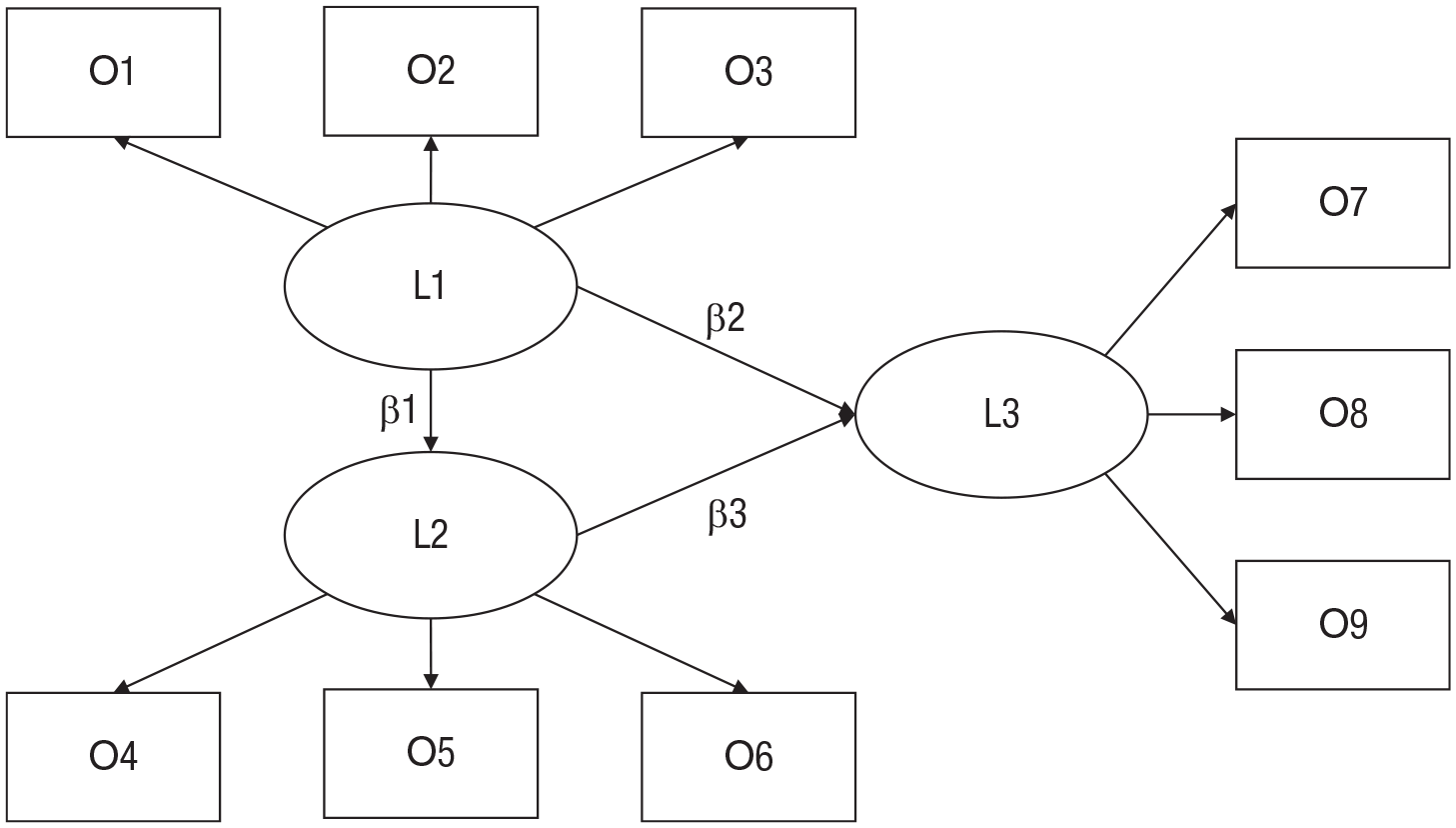
High-dimensional theoretical model for the example study discussed in the text. Rectangles indicate observed variables, which are denoted as “O#,” and ovals indicate latent variables, which are denoted as “L#.” The focal coefficient is β2. We omitted visualizations of error terms for simplicity.
Assume that a research team’s theoretical model looks as depicted in Figure 5 and the focal hypothesis is that in the incoming sample of 402 participants, there will be a positive small-to-medium effect of L1 on L3 (say, β between 0.15 and 0.35; we ignore p values in this example). However, the true (population-level) data-generating process has a negative beta coefficient (β = −0.1). In the full data set of 402 participants (see the materials on OSF for data and scripts), the researchers indeed find a beta value of 0.178. They conclude that their initial prediction was correct, but wonder whether their conclusion might have been distorted by a small group of observations in their sample given that a different research group had suggested previously that the relationship could be negative (β between −0.15 and −0.35). Thus, the current group uses StatBreak to investigate whether a coefficient of −0.15 or lower would have actually been in line with their data had it not been for some special data points.
When feeding their own data and model into StatBreak, they find that deleting the last two observations indeed leads to a negative beta coefficient (β = −0.170). Thus, they can conclude that the last two collected observations fully flip the effect that would have been observed for the first 400 participants, and that they should certainly examine the nature of these two observations.
Criteria for Evaluating Robustness
The StatBreak algorithm provides output indicating that deleting certain cases (e.g., Observations 15, 19, 209, 664, and 954) entails a certain value for the target statistic (e.g., r < .1). However, this output needs to be evaluated regarding its implications for the robustness of the initial conclusion. Two main criteria have to be considered to ascribe a label such as “high robustness” or “limited robustness” to a data-based conclusion: first, the nature of the observations that would need to be excluded to lead to a different conclusion and, second, the number of such observations. When it comes to interpreting numerical tests (in this case, robustness tests), it is tempting to generate a set of strict conventions to simplify the process (e.g., p < .05 → “significant”; r > .70 → “reliable”; for criticism, see, e.g., Lakens et al., 2018). Similarly, it is tempting to generate rules of thumb for how few excluded cases are too few for an initial conclusion to be called robust. However, we are reluctant to recommend a one-size-fits-all approach, given the numerous factors that influence the proportion of exclusions needed to generate reliable cutoff values. These factors include sample size, effect size, variable distributions, model complexity, test statistic, and the statistic’s goal value. Further, as noted earlier, the arbitrary nature of alternative rules of thumb appears to be partly responsible for the neglect of case analyses in applied research.
We assume that the nature of potentially excluded cases is more informative than the sheer number of such cases, unless the absolute number of exclusions required for a qualitatively different finding is very small (e.g., an effect crosses a justified threshold after only one or two observations are excluded). In such a case, the initial conclusion is certainly not robust. Notice that despite such low robustness of a conclusion, the result might still be numerically robust (e.g., with the exclusions, the p value might change from .049 to .051) or not robust (e.g., a change from .005 to .3). StatBreak focuses on the robustness of conclusions and not on numerical robustness, which is apparent in that users have to indicate the goal value for their target statistic (i.e., the value that would cause their initial conclusion to change). Low robustness of an initial conclusion is often easy to anticipate when initial results already lie close to justified cutoffs, which is common in the case of binary or categorical conclusions (cf. the predictive power of p values for replication success: Altmejd et al., 2019).
When one is inspecting the nature of potentially excluded cases, the critical question is whether there is reason to believe that these observations are particularly unusual (Judd, McClelland, & Culhane, 1995), belong to a different population than the rest of the sample does (Aguinis, Gottfredson, & Joo, 2013), or somehow contaminate the sample statistics (Bakker & Wicherts, 2014b). For example, such observations may involve measurement errors, nonattentive participants, data collected by a different person, data collected in a different setting, or any other factor that makes them noteworthy. Nonrobust findings may also arise through questionable research practices, such as optional stopping, optional covariates, or motivated outlier exclusions, which allow researchers to tune their studies’ outcome statistics. Accordingly, StatBreak is likely to flag nonrobustness in such cases (for simulations, see the materials on OSF). In the next section, we give a detailed example of applying StatBreak to real data from psychological research and investigating the nature of observations flagged for exclusion.
Applying StatBreak to Real Data
Given that the StatBreak algorithm worked as intended with simulated data, we went on to test its usefulness on real data from an unpublished study in which we investigated the relationship between online language and dispositional trust. We recruited a sample of 398 Twitter users who provided their most recent 200 tweets and filled out a questionnaire measure of dispositional trust (Yamagishi & Yamagishi, 1994). In these data, we found a significant negative correlation between dispositional trust and the frequency with which participants talked about themselves in their tweets (measured by their use of personal pronouns, such as I or me), r(396) = −.12, p = .018. This finding is consistent with a theory that ascribes more social intelligence to people with high dispositional trust, and describes people with low dispositional trust as relatively self-focused and nonempathic (Raskin & Shaw, 1988; Yamagishi, Kikuchi, & Kosugi, 1999).
After initially concluding that we had found a significant negative correlation, we used StatBreak to examine which (and how many) observations would need to be deleted to conclude that the effect was not significant. In the applications of StatBreak presented thus far, we always chose p > .05 as the cutoff for a positive conclusion, as it is the most common alpha level used in psychological research. However, as is true for alpha levels, numeric goal values for StatBreak are not set in stone; rather, they should be justified by the researcher (Lakens et al., 2018). More precisely, when assessing the robustness of one’s conclusion using StatBreak, one needs to be aware of how one’s conclusion maps onto the observed statistic. For instance, we could interpret the observed p value of .018 in our study similarly to the way in which we would interpret a p value of .03 (or maybe even .051) and conclude that there is a small, but certainly not tiny, chance that such data, or more extreme data, would occur if there is no real correlation. Conversely, if we had observed a p value of .1, our initial conclusion certainly would have been qualitatively different (i.e., that there is a pretty good chance that such data would occur if there is no real correlation). For this example, we chose p > .10 as StatBreak’s conservative goal value in order to emphasize that researchers should justify how their conclusions map across target statistics (instead of following numerical conventions). Notice that such conclusion cutoffs (in this case, the alpha level) are much more convincing if their justification is preregistered, as this limits their exploitation for questionable research practices (albeit not the often-unsatisfactory practice of dichotomizing or categorizing conclusions). For the relationship between dispositional trust and self-referencing, StatBreak found a solution with three case exclusions that satisfied the criterion of p > .10. As the analysis involved only two variables in this case, the results can be depicted in a scatterplot (see Fig. 6).
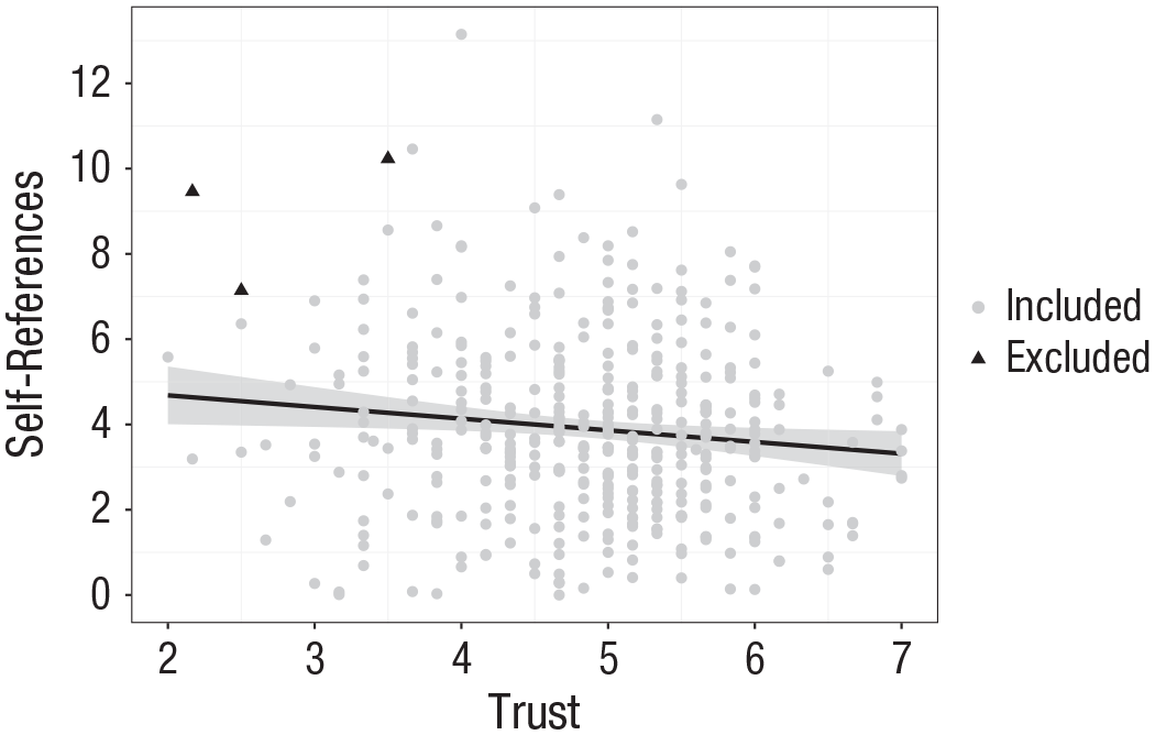
Results for the application of StatBreak to real data. The scatterplot (with best-fitting full-sample regression line) shows the negative relationship between the usage of self-references in tweets and dispositional trust in the full data set. However, StatBreak flagged three data points (black triangles) whose exclusion from the sample would render the effect nonsignificant, p > .10. The gray band shows the 95% confidence interval.
Although the relatively small number of case exclusions could be interpreted as indicating that our initial conclusion is not robust, it is not sufficient to simply note the number. Most small effects found in nonlarge samples disappear when a few selected cases are excluded (see Fig. 4), and when we simulated a case with a population-level correlation of .12 and a total sample of 398, StatBreak indicated that we would need to delete a median of 4 observations to change our conclusion, so it is not necessarily noteworthy that StatBreak flagged 3 observations in the real data. More important is an assessment of the nature of the flagged cases, as prescribed by virtually all techniques for analyzing influential cases (Barnett, 1978; Osborne & Overbay, 2004).
In Figure 6, the three potentially excluded data points are somewhat outlying, but not sufficiently so to look suspicious per se. However, one of the three flagged Twitter accounts had a high rate of self-referencing because it constantly posted the same, apparently non-self-authored, advertisement texts including the words I and me (a paraphrased example: “I am winning cash! Come join me under this URL!”). We reasoned that such tweets result from a special data-generating process, which warrants an exclusion. The tweets of both other flagged accounts did not look suspicious, and because we could not see any quantitative or qualitative reason to exclude them (both accounts posted tweets with varied wording and noncommercial content), we left them in the sample. When the one suspicious case was excluded, the new result, r = −.11, p = .029, was quite close to the original result.
Additionally, we next made use of our new knowledge and searched across the whole range of trust scores for other spam accounts with similarly high frequencies of self-referencing (i.e., the search was not biased toward the null hypothesis and against interesting findings). When we excluded 4 similar spam accounts (which also constantly reposted advertisement texts), the correlation remained negative, r = −.093, p = .066. Notice that StatBreak did not highlight these additional cases because it merely indicates the luckiest observations, not the observations that are qualitatively suspicious given certain rules (in this case, posting of repetitive, commercial content). StatBreak itself does not provide a qualitative review of each data point, and it also will not highlight nonoutlying data points. In this case, it merely alerted us to the luckiest data points (repetitive wording led to their extreme scores), and our manual inspection led to the insight that repetitive accounts are sometimes spam accounts. A future study could preregister an exclusion rule to discard data from such accounts. Given that we judged the sample without the spam cases to be more informative, we might adjust our estimated probability of the data (or more extreme data) under the null hypothesis, characterizing it as somewhat small (p = .066), rather than small (p = .018). Thus, we would argue that the original result appears to have been slightly distorted by a small number of suspicious data points, only one of which was highlighted by StatBreak because of its strong contribution to the initial results. This approach to finding suspicious influential cases involves a combination of automatic computation (in this case, computation by a genetic algorithm; in other cases, computation of outlier metrics) and researchers’ judgment regarding the flagged cases, both of which are required for virtually any method of analyzing influential cases.
Advantages of StatBreak
In this section, we highlight advantages of StatBreak over popular existing methods.
Breadth of applicability
Methods of dealing with outliers and influential data points are often bound to certain types of statistical models. For instance, Cook’s (1977) D is designed for regression models, and rules such as “exclude everything more than 3 SD from the mean” have to be applied to univariate continuous data. Similarly, robust-modeling alternatives are tailored to specific statistical analyses (Field & Wilcox, 2017). Having to tailor one’s strategy for examining outliers to the specifics of each analysis is burdensome, and a universally applicable tool like StatBreak can therefore be useful.
Popular outlier metrics can alert researchers that specific statistics of interest might be distorted. For instance, DFBETAS and DFFITS target, respectively, how much individual observations influence beta coefficients and predicted values (Cousineau & Chartier, 2010), whereas standardized residuals target prediction errors. However, such metrics might focus on statistics that are not the crucial, conclusion-relevant statistic that needs to be examined for distortion by lucky observations. An observation might, for instance, distort the beta coefficient of a linear regression model, while having little effect on the explained variance or the intercept. In StatBreak, researchers have to explicitly specify which statistic is crucial for their conclusions, and StatBreak will search data points relevant for this statistic.
Further, when using popular outlier metrics, researchers frequently have to make decisions based on cutoff scores. However, many find it difficult to justify a cutoff score given their lack of experience with, for example, Cook’s D, Studentized residuals, or Mahalanobis distance and thus blindly rely on conventional rules of thumb. StatBreak does not eliminate this issue, but it allows researchers to base conclusions on metrics that they are more familiar with, helping them to make better-informed decisions. For instance, we assume that it is more difficult for researchers to decide whether a Cook’s D of 3 is problematic than to decide whether it is problematic that excluding Observations 7 and 24 reduces an effect size by 75%. Although StatBreak clearly does not solve the issue of subjectivity in cutoffs, it allows researchers to calibrate their confidence in a way they can justify themselves. Further, StatBreak guides researchers toward qualitative instead of purely quantitative case analyses, as we discuss later.
Thorough search
To effectively test for multiple influential observations, researchers must test for outliers in a stepwise procedure (as single-step procedures cannot detect outliers masked by other outliers; Bendre & Kale, 1985). However, manually excluding the most outlying case and recomputing the outlier analysis in the new subsample, in an iterative process, is burdensome, leading researchers to compute outlyingness scores once (greedy search) and exclude cases based on these scores. StatBreak automates the stepwise approach, which helps researchers find masked outliers that would have been overlooked in nonstepwise analyses.
Further, high-dimensional data might not allow the application of some metrics and plots that can be used to find outliers. Although there are special methods for such data (Caussinus, Fekri, Hakam, & Ruiz-Gazen, 2003), applied researchers might be even more reluctant to conduct such analyses given the increased effort required to learn and apply these methods. Conversely, the application of StatBreak does not differ between high- and low-dimensional problems, and StatBreak is therefore a simple tool for dealing with complex models (see the section titled Using StatBreak for High-Dimensional Models).
Qualitative analyses and explicit links between statistics and conclusions
Simple methods, such as excluding the top and bottom 2% of cases or excluding everything with a Cook’s D higher than x, can be carried out as automatic decision rules, which do not require reflection on the nature of the excluded cases (e.g., “why were they so extreme?”). StatBreak’s output (indicating, e.g., that deleting Observations 3 and 5 from the data leads to a different conclusion, given the specified criterion) does not state that the flagged cases should be deleted. Given that they appear to be crucial, and that their level of suspiciousness is to be determined, we believe that users are effectively nudged toward finding out what is special about these observations. However, it is also noteworthy that this traditionally encouraged qualitative outlier review can entail ad hoc storytelling, which can be misused as a questionable research practice. In the case of StatBreak, for example, a user might say, “StatBreak suggests that deleting Observation 42 results in a much smaller effect size, but we decided to leave this data point in because we do not think it is suspicious.” When faced with incomplete and nonconvincing applications of StatBreak, reviewers should run the algorithm themselves to assess whether StatBreak’s output was indeed not worrisome.
StatBreak not only nudges users toward in-depth review of individual cases, but also facilitates explicit links between primary analyses and conclusions. Many publications present conclusions based on numerical results. A conclusion is often based on a single number: for example, “we believe that there is a treatment effect because the statistical test yielded a p value of .001,” or “we believe that the model makes good predictions because the model’s R2 is .65.” Often, the worry regarding outliers is that the conclusion would have changed had these special data points been considered. To consider alternative conclusions, researchers need to be aware how their conclusions map out across alternative values of the target statistic (e.g., Funder & Ozer, 2019). StatBreak requires users to make this mapping explicit by indicating a value under which their conclusion would have differed.
Summary
In summary, StatBreak is a tool that offers advantages in applicability, thoroughness, and facilitation of reflection on outliers. However, we emphasize again that this R-based tool is not supposed to replace well-established methods. Popular metrics are informative about the precise outlyingness of data points (StatBreak is not), and robust estimation methods guard against assumption violations beyond the presence of outliers.
Example Usage of the StatBreak R Package
In R, the StatBreak package can be downloaded though the command
Running this code yields the following output (trimmed):
. . .
As is evident in the output, StatBreak finds the optimal solution within the first generation of subsamples. StatBreak indicates that discarding a single observation lets the focal p value jump from .040 to .342. The generated
In addition to the functionality we have already described, the package includes a function for excluding lucky groups of observations (i.e., higher-level clusters, such as schools or experimental conditions).
Regardless of whether the statistic of interest result from a linear regression, a multilevel model, a meta-analysis, or any other procedure, StatBreak requires only one or two lines of code more than the original analysis. Adding the
Discussion
Whether an interesting sample statistic is caused by individual observations is a long-standing concern in psychological research. We have introduced a new method to find and count cases that strongly contribute to a finding. This search is based on a genetic algorithm. In contrast to related strategies, such as robust modeling, outlier metrics, and visual inspection, the new method is applicable to any analysis. Further, it is straightforward to apply, encourages qualitative data review, requires explicit links between statistics and conclusions, and provides very readable outputs (identifying observations that would need to be deleted to obtain a noninteresting finding). Thus, in contrast to other techniques for analyzing influential cases, the current method is designed specifically for inquiring whether individual observations caused an interesting finding.
We encourage researchers and reviewers to engage in study-specific discussion of the number and nature of excluded cases when they interpret the robustness of findings. We believe that such deliberations are very beneficial, as they nudge researchers and reviewers to engage with the data on a deeper level and calibrate their confidence in the obtained findings. We again want to mention that StatBreak is biased against findings that support researchers’ hypotheses and therefore does not remove bias from data. Other methods—most prominently, preregistered criteria for excluding outliers—are better suited to achieve this goal. Further, StatBreak is not intended to heighten the bar for empirical findings by imposing a new robustness criterion. Rather, StatBreak serves as a simple tool for researchers and reviewers who want to ascertain whether spectacular findings were due to a small number of outliers in the data.
Supplemental Material
Rosenbusch_Rev_Open_Practices_Disclosure – Supplemental material for StatBreak: Identifying “Lucky” Data Points Through Genetic Algorithms
Supplemental material, Rosenbusch_Rev_Open_Practices_Disclosure for StatBreak: Identifying “Lucky” Data Points Through Genetic Algorithms by Hannes Rosenbusch, Leon P. Hilbert, Anthony M. Evans and Marcel Zeelenberg in Advances in Methods and Practices in Psychological Science
Footnotes
Acknowledgements
We thank Michèle Nuijten and Joachim Krueger for their thoughtful comments and guidance.
Transparency
Action Editor: Daniel J. Simons
Editor: Daniel J. Simons
Author Contributions
H. Rosenbusch and L. P. Hilbert jointly generated the idea for the study. H. Rosenbusch coded the R package and analyses. H. Rosenbusch, L. P. Hilbert, and A. M. Evans examined the accuracy of those analyses. All the authors participated in writing and critically editing the manuscript. All the authors approved the final submitted version of the manuscript.
Notes
References
Supplementary Material
Please find the following supplemental material available below.
For Open Access articles published under a Creative Commons License, all supplemental material carries the same license as the article it is associated with.
For non-Open Access articles published, all supplemental material carries a non-exclusive license, and permission requests for re-use of supplemental material or any part of supplemental material shall be sent directly to the copyright owner as specified in the copyright notice associated with the article.