Visualization of Brain Statistics With R Packages ggseg and ggseg3d

Abstract

There is an increased emphasis on visualizing neuroimaging results in more intuitive ways. Common statistical tools for dissemination of these results, such as bar charts, lack the spatial dimension that is inherent in neuroimaging data. Here we present two packages for the statistical software R that integrate this spatial component. The ggseg and ggseg3d packages visualize predefined brain segmentations as 2D polygons and 3D meshes, respectively. Both packages are integrated with other well-established R packages, which allows great flexibility. In this Tutorial, we describe the main data and functions in the ggseg and ggseg3d packages for visualization of brain atlases. The highlighted functions are able to display brain-segmentation plots in R. Further, the accompanying ggsegExtra package includes a wider collection of atlases and is intended for community-based efforts to develop additional compatible atlases for ggseg and ggseg3d. Overall, the ggseg packages facilitate parcellation-based visualizations in R, improve and facilitate the dissemination of results, and increase the efficiency of workflows.

Visualization is increasingly important for accurate explanation and interpretation of neuroimaging results, as current research is able to generate a large amount of raw data and outcomes. For MRI, neuroimaging software provides whole-brain information by dividing space into many small units (> 100.000). Nonetheless, these data are often grouped and summarized using a limited number of regions in predefined brain-parcellation atlases. Brain parcellations segment the brain into a finite set of meaningful neurobiological components, each of which reflects one or more brain features based on either structural or connectivity properties (Eickhoff, Yeo, & Genon, 2018). The use of brain atlases in neuroscience is widespread, as they facilitate interpretation and minimize the amount of data (in comparison with whole-brain data), and hence reduce statistical problems with multiple comparisons. This enables replicability and data sharing in the case of otherwise computationally expensive analyses, which are often performed in specialized software environments, such as R (R Core Team, 2019).

MRI data provide good spatial resolution, and thus an optimal representation has to respect spatial relationships across regions. Results from brain-atlas analyses are most meaningfully visualized when projected onto a representation of the brain, so it is desirable for any visual representation to take spatial relations into account. Such projections provide clear points of reference (especially when the reader is unfamiliar with the atlas), improve readability, guide interpretation, and convey the spatial patterns of the data. Adopting the grammar of graphics implemented in ggplot2 (Wickham, 2016), one can plot neuroimaging data directly in R with several tools, such as ggBrain (Fisher, 2019) and ggneuro (Muschelli, 2017; see Muschelli et al., 2019, for curated neuroimaging packages for R). Yet these tools display whole-brain image files and are not well suited for representing brain-atlas data.

In this Tutorial, we introduce two packages for visualizing brain-atlas data in R. The ggseg and ggseg3d packages—plus the complementary ggsegExtra package—include precompiled data sets for different brain atlases that allow for 2D and 3D visualization. The 2D functionality in ggseg is based on polygons and ggplot2-based grammar of graphics (Wickham, 2016), whereas the 3D functionality in ggseg3d is based on tri-surface mesh plots and plotly (Sievert, 2019).

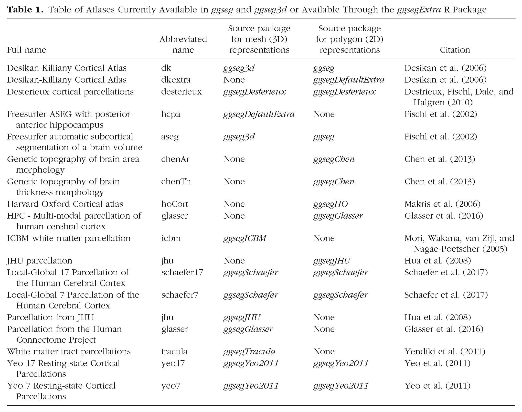
In addition to the compiled data sets, the ggseg and ggseg3d packages provide tailored functions that allow brain-data integration and plotting, as well as other minor features, such as custom color palettes. The data featured in the packages are derived from two well-known parcellations: the Desikan-Killiany cortical atlas (dk; Desikan et al., 2006), which covers the cortical surface of the brain, and the Automatic Segmentation of Subcortical Structures (aseg; Fischl et al., 2002), which covers the subcortical structures. Both atlases are implemented in a variety of neuroimaging software, such as FreeSurfer (Dale, Fischl, & Sereno, 1999; Fischl & Dale, 2000; Fischl, Sereno, & Dale, 1999), and are commonly used to study developmental changes, disease biomarkers, genomic data, and cognition (Amlien, Sneve, Vidal-Piñeiro, Walhovd, & Fjell, 2019; Pizzagalli et al., 2009; Walhovd et al., 2005). The ggsegExtra package contains a list of online repositories of precompiled atlases (currently 11 additional polygon atlases and 10 additional mesh atlases), and it is frequently updated. A summary of all available atlases compatible with the ggseg packages as of June 2020 can be found in Table 1.

Table 1.

Table of Atlases Currently Available in ggseg and ggseg3d or Available Through the ggsegExtra R Package

Full name	Abbreviated name	Source package for mesh (3D) representations	Source package for polygon (2D) representations	Citation
Desikan-Killiany Cortical Atlas	dk	ggseg3d	ggseg	Desikan et al. (2006)
Desikan-Killiany Cortical Atlas	dkextra	None	ggsegDefaultExtra	Desikan et al. (2006)
Desterieux cortical parcellations	desterieux	ggsegDesterieux	ggsegDesterieux	Destrieux, Fischl, Dale, and Halgren (2010)
Freesurfer ASEG with posterior-anterior hippocampus	hcpa	ggsegDefaultExtra	None	Fischl et al. (2002)
Freesurfer automatic subcortical segmentation of a brain volume	aseg	ggseg3d	ggseg	Fischl et al. (2002)
Genetic topography of brain area morphology	chenAr	None	ggsegChen	Chen et al. (2013)
Genetic topography of brain thickness morphology	chenTh	None	ggsegChen	Chen et al. (2013)
Harvard-Oxford Cortical atlas	hoCort	None	ggsegHO	Makris et al. (2006)
HPC - Multi-modal parcellation of human cerebral cortex	glasser	None	ggsegGlasser	Glasser et al. (2016)
ICBM white matter parcellation	icbm	ggsegICBM	None	Mori, Wakana, van Zijl, and Nagae-Poetscher (2005)
JHU parcellation	jhu	None	ggsegJHU	Hua et al. (2008)
Local-Global 17 Parcellation of the Human Cerebral Cortex	schaefer17	ggsegSchaefer	ggsegSchaefer	Schaefer et al. (2017)
Local-Global 7 Parcellation of the Human Cerebral Cortex	schaefer7	ggsegSchaefer	ggsegSchaefer	Schaefer et al. (2017)
Parcellation from JHU	jhu	ggsegJHU	None	Hua et al. (2008)
Parcellation from the Human Connectome Project	glasser	ggsegGlasser	None	Glasser et al. (2016)
White matter tract parcellations	tracula	ggsegTracula	None	Yendiki et al. (2011)
Yeo 17 Resting-state Cortical Parcellations	yeo17	ggsegYeo2011	ggsegYeo2011	Yeo et al. (2011)
Yeo 7 Resting-state Cortical Parcellations	yeo7	ggsegYeo2011	ggsegYeo2011	Yeo et al. (2011)

This Tutorial introduces the ggseg, ggseg3d, and ggsegExtra packages and familiarizes the reader with the main functions and the general use of the packages. We focus on the two main functions: ggseg() for plotting 2D polygons and ggseg3d() for plotting 3D brains based on tri-surface mesh plots. The Tutorial complements the package documentation and vignettes that can be found online for all three packages: ggseg (https://lcbc-uio.github.io/ggseg), ggseg3d (https://lcbc-uio.github.io/ggseg3d), ggsegExtra (https://lcbc-uio.github.io/ggsegExtra). These online materials provide additional information not covered here.

Disclosures

All materials for this Tutorial, including the R Markdown document used to write it, may be found online at https://github.com/Athanasiamo/ggsegpaper.

Plotting Polygon Data (ggplot2)

The main function for plotting 2D data is ggseg() from the ggseg package. By default, the function automatically plots the dk atlas (see Fig. 1). The ggseg() function is a wrapper for geom_polygon() from ggplot2 (Wickham, 2016), and it can be built upon and combined in the same way as any ggplot object. The image plot consists of a simple brain representation containing no extra information. Hence, ggseg plots can be easily complemented with any of the available ggplot2 features and options. We recommend that users get familiarized with ggplot2. The ggseg package is currently available only through GitHub, but we expect to submit it to the Comprehensive R Archive Network (Hornik, 2012) in early 2021.

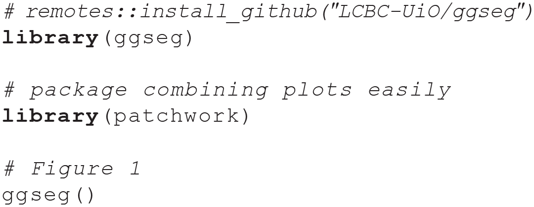
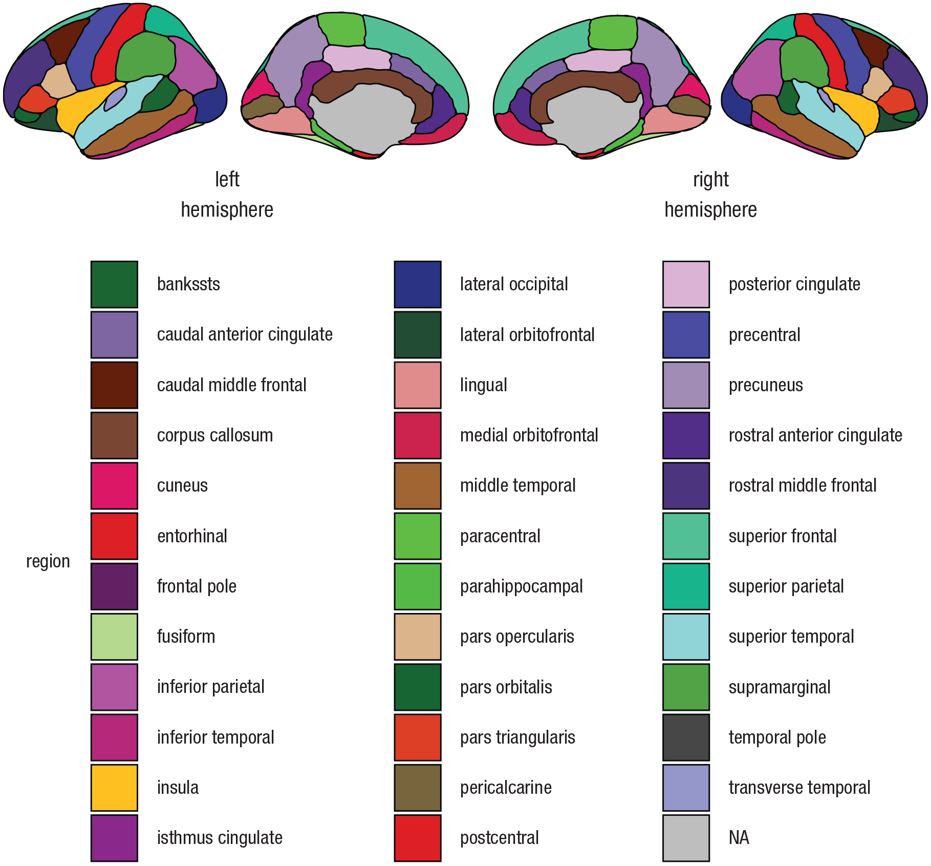
To start the Tutorial, use the following code, which loads the necessary R libraries and plots the dk atlas using ggseg (Fig. 1):

Fig. 1.

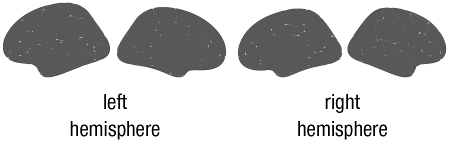
Plot of the Desikan-Killiany atlas (Desikan et al., 2006) in gray polygons. This plot was created by running the ggseg() function without any additional arguments.

In addition to the standard options for ggplot2 polygon geoms, the function has several options for plotting the main brain representations. These options are atlas-specific. For cortical atlases, such as the dk, one can stack the hemispheres, display only the medial or lateral side, choose either one or both hemispheres, or choose any combination of hemisphere and view (see Fig. 2 for examples). For subcortical atlases, such as the aseg atlas, the options are more limited, but one can often choose among axial, sagittal, and coronal views. The following code produces the six different ways of customizing ggseg plots illustrated in Figure 2:

Fig. 2.

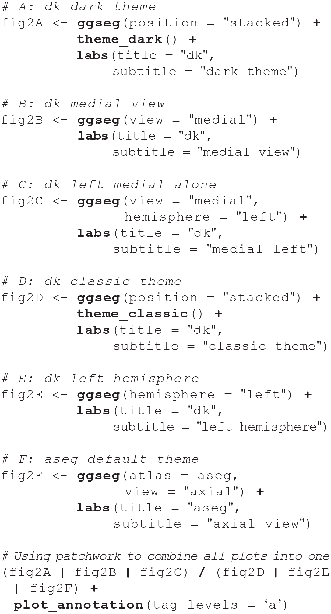
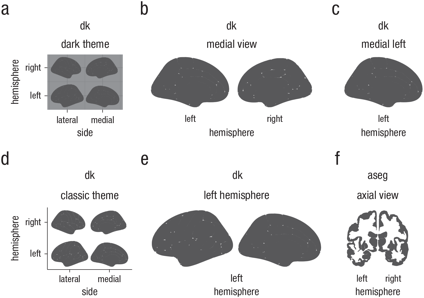
Illustration of some ggseg display options for cortical atlases. The displays here are representations of (a) the Desikan-Killiany (dk) atlas (Desikan et al., 2006), stacked, with the dark theme; (b) the dk atlas with the medial view only; (c) the dk atlas with only the left medial display; (d) the dk atlas, stacked, with the classic theme; (e) the dk atlas with the left hemisphere only; and (f) the axial view of the Automatic Segmentation of Subcortical Structures (aseg atlas; Fischl et al., 2002).

Using one’s own data with fill and colour

The ggseg() function accepts any argument you can supply to geom_polygon() and therefore is easy to work with for users familiar with ggplot2 functionality. Standard arguments like fill, which floods the segments with color, or colour, which colors the edges around the segments, are typical arguments to provide to the function either as a single setting value or within the ggplot2 mapping function aes. To use color palettes corresponding to those used in the original neuroimaging software, one can use atlas-specific palette scales that are derived from the original publications introducing the segmentation. Figure 3 illustrates how the atlas polygons can be filled with differentiating colors according to the region names in the atlas being used and with the color palette for that atlas (in this case, dk). It is produced by the following code:

Fig. 3.

Plot created by supplying region to the fill option in ggseg() to create a discrete color palette over the segments in the Desikan-Killiany atlas (Desikan et al., 2006). The default palette of this atlas, illustrated here, corresponds to the FreeSurferColorLut scheme.

Most users will use ggseg() to display, with a color scale, some descriptive or inferential statistics, such as mean thickness of different brain regions or their relationships to cognition. Yet before projecting the statistics onto the segments, users should explore the structure of the atlas data sets. The atlas data-set structure will help users understand what incoming statistical data need to look like. Note that each atlas corresponds to a unique data set. All the data sets have similar structures, and each contains key information regarding the atlas, the region names, and the coordinates for the segment polygons. One can use the following code to inspect the first five rows of atlas data:

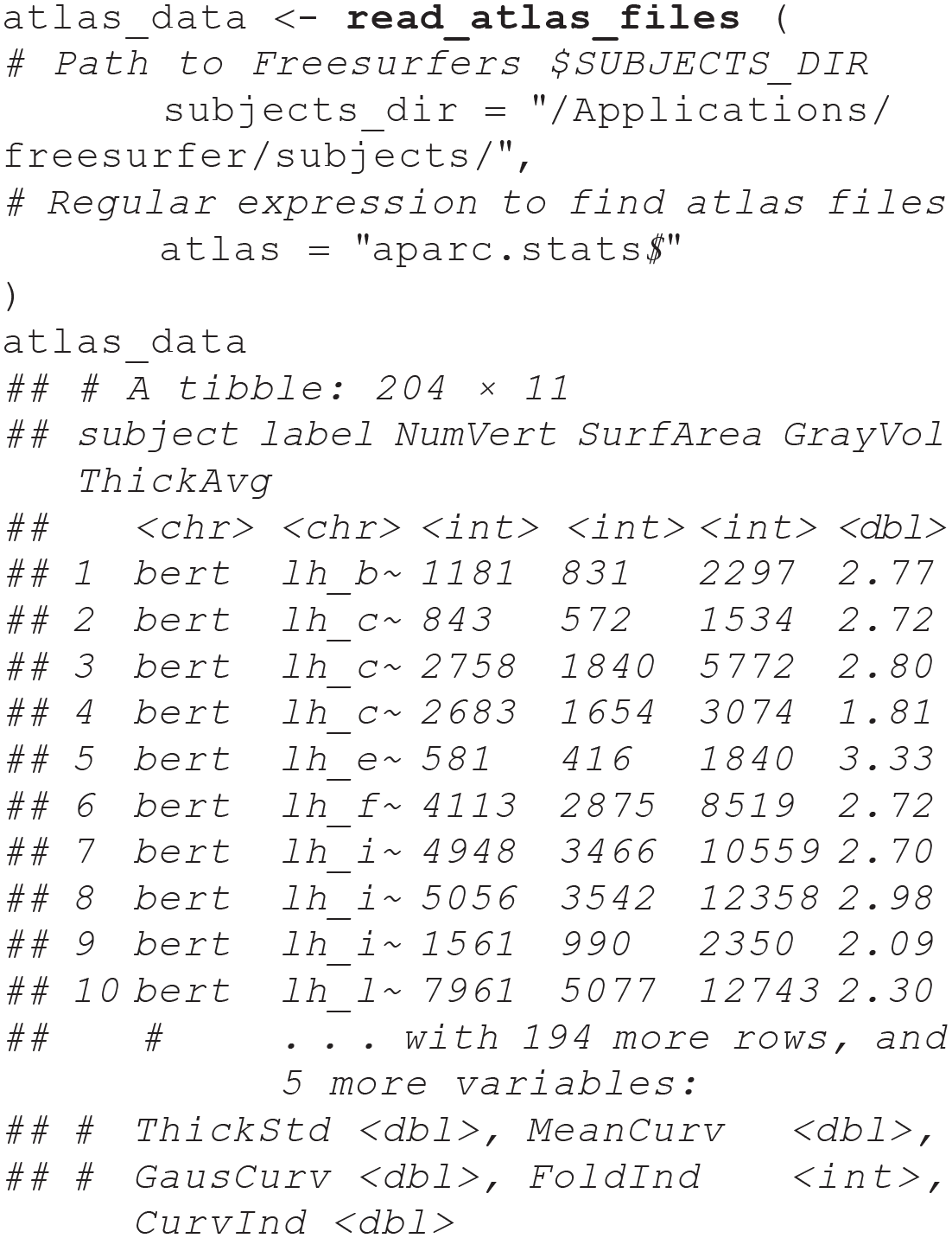
In any atlas, the column label is particularly useful for combining the data of interest with the ggseg polygons. This column contains the label (region) names from the original neuroimaging software. For example, the label column in the dk atlas matches the region names from FreeSurfer’s statistics table outputs. Yet the data in ggseg are in long format; that is, each region has a single row. Any data of interest need to be in this same format, but often data sets are organized in wide format, in which subjects are represented by rows and each data variable is represented in a separate column. Such data sets need to be rearranged to work with ggseg. Summary statistics files from FreeSurfer have a file format that can be difficult to work with in R. In a set of functions in ggseg, we facilitate conversion between FreeSurfer data and ggseg-compatible data. An extended online vignette of the various options using these functions is available online (https://lcbc-uio.github.io/ggseg/articles/freesurfer_files.html). The following code is an example of this conversion. It imports summary data that have been compiled using FreeSurfer’s asegstats2table (volumes), but it can also handle reading in data from aparcstats2table (for surfaces):

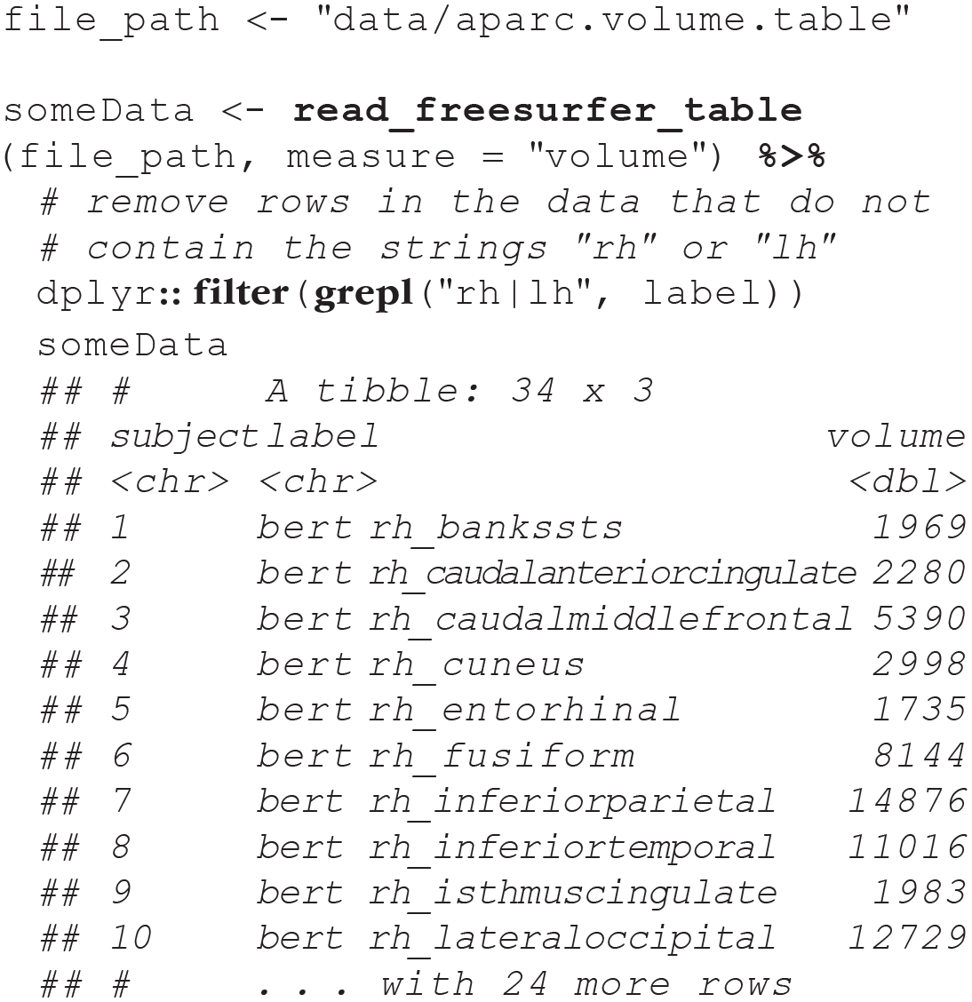
These summary stats files also contain extra metrics, such as intracranial volume and total gray-matter volume. These latter measures do not map onto ggseg, and therefore, one should filter them out of the data returned from read_freesurfer_table (as the preceding example code does in the filter step).

A second option is to read in statistics files directly from the entire subject directory, using regular expression to select the statistics files from the target atlas. The default aparc (FreeSurfer’s name for the dk atlas) has a unique string ending with aparc.stats, which one can use to read in all subject statistics for that particular atlas. One can filter specific subjects and/or regions from the R object data.frame. The following code provides an example of how to use the read_atlas_files function to read in all FreeSurfer statistics files for a specific atlas from all subjects in the FreeSurfer subject directory:

These long-format data can be used directly with the ggseg()function, as the label column corresponds in name and content with the label column in the dk atlas’s data. The data must include a column that has the same column name and at least some data matching the values in the corresponding column in the atlas’s data. In the following code segment, the ggseg()function will recognize the matching column label and merge the supplied data into the atlas using dplyr joins. The appearance of the plot can then be modified in the same ways as any other ggplot2 graphs, using functions such as scales, labs, and themes, as illustrated in Figure 4, which is produced by the following code:

Fig. 4.

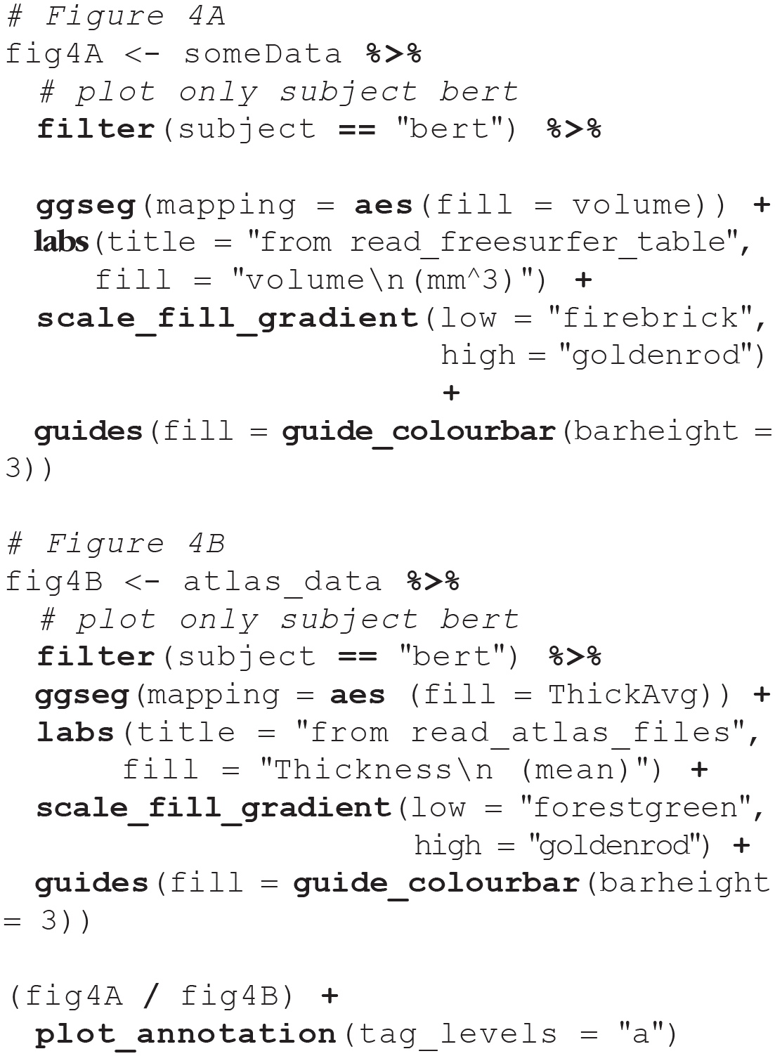
Examples of outputs obtained using ggseg() with data supplied through the .data option. This enables the use of columns in the supplied data as aesthetic arguments (such as fill). The ggseg plot can be used with any other polygon-compatible function from ggplot2 or ggplot2 extensions, for instance, the standard ggplot2 functions for adding a title, changing the legend name, and changing the color scheme. The example in (a) shows plots created by data supplied to ggseg through the .data argument with a single hemisphere specified and with a color scheme ranging from red to gold specified through the scale_fill_gradient function. The example in (b) shows plots created by data supplied to ggseg through the .data argument with no hemisphere information and a color scheme ranging from green to yellow specified through the scale_fill_gradient function.

If the results are only in one hemisphere, but you still want to plot both of them, make sure your data.frame includes the column hemi with either right or left. In such cases, data will be merged into the atlas both by region and by hemi. The online documentation contains more detailed information about how to adapt data and view only one hemisphere or side.

Creating subplots

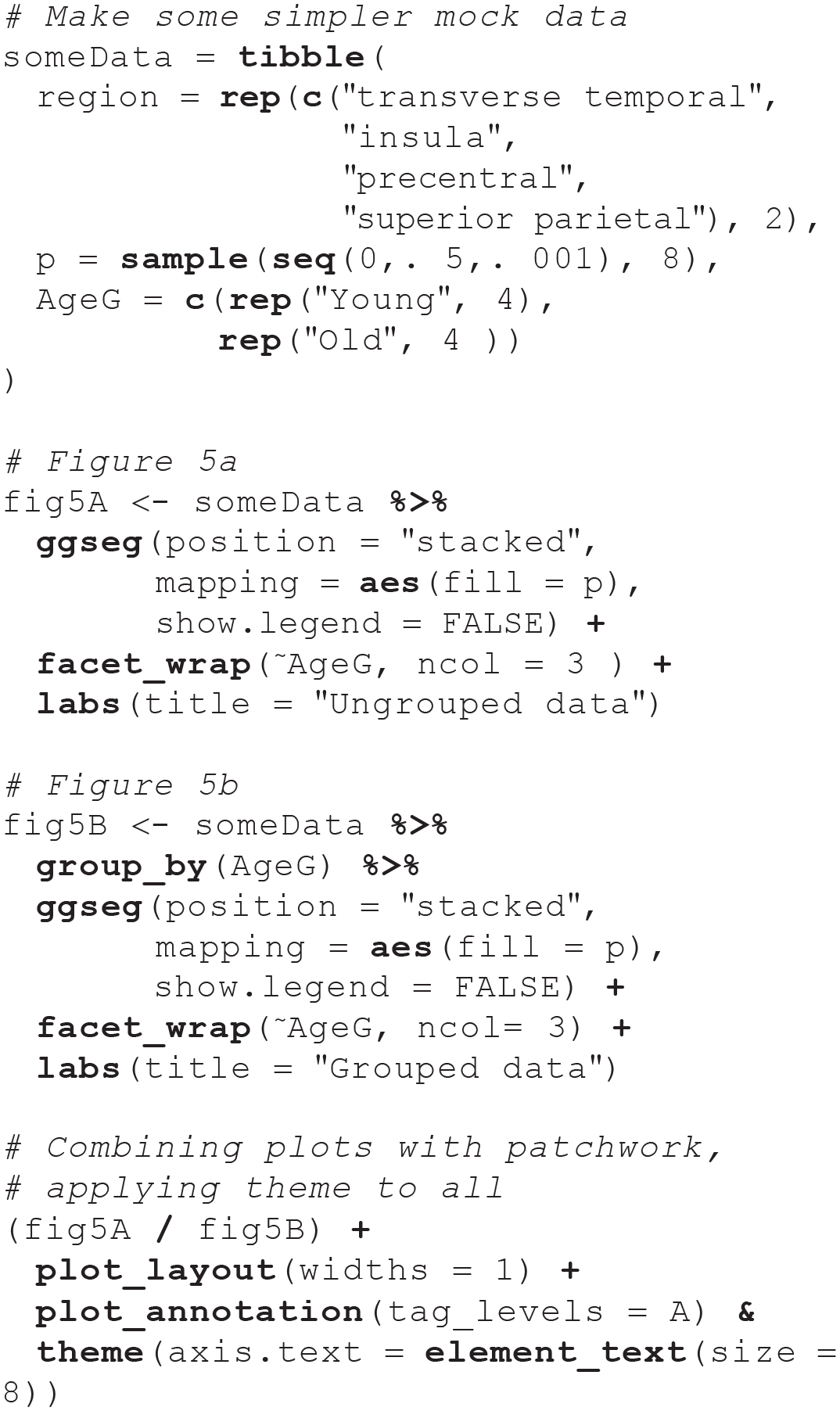
There is often the need to plot a statistic of interest in different groups (e.g., to plot thickness or brain-cognition relationships separately in young and older adults). This may be accomplished with ggseg(), using ggplot2’s facet_wrap or facet_grid function. To create such plots, three steps need to be followed:

1. Convert the data to long format with a column indexing which group each row corresponds to (group data should appear in separate rows, not in separate columns).

2. Use dplyr’s group_by() function to group the data

3. Finally, apply facet_wrap or facet_grid. The ggseg()function will detect the grouped data and adapt it to facet’s requirements.

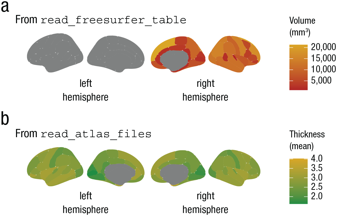
Figure 5b provides an example of separate subplots created following these three steps. In this example, ggseg was applied to a mock data set including summary statistics for groups labeled “Young” and “Old.”

Fig. 5.

Examples of incorrect and correct faceting with ggseg. The plots in (a) were created using ungrouped data. The data were faceted incorrectly because they were not merged correctly with the atlas. In contrast, when the data were grouped (b), they merged in the expected way, and correctly faceted plots were created. NA = not applicable or not represented in the data.

The second step is needed because the ggseg()function is a ggplot wrapper rather than an extension, and thus has a particular structure and pipeline for combining the atlas with supplied data. Figure 5a shows the result when ggseg was applied to the same mock data set, but with the data ungrouped. Note that the data were combined incorrectly, so there are three subplots rather than two. Regions not represented in the data (“NA”) have their own subplot; the other two subplots include only regions with valid data.

The following code was used to create the plots in Figure 5:

Using other atlases

Although the dk atlas is the default atlas for the ggseg() function, this function can also create visualizations of other compatible atlases through the atlas argument. As mentioned in the introduction, the aseg subcortical atlas comes with the package. The procedure for the aseg atlas is the same as the procedure for the dk atlas except for the hemisphere argument, which is superfluous in subcortical-atlas visualizations. The following code segment, which produces the plots in Figure 6, is an example of how to plot the aseg subcortical atlas:

Fig. 6.

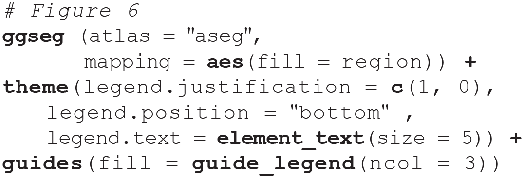
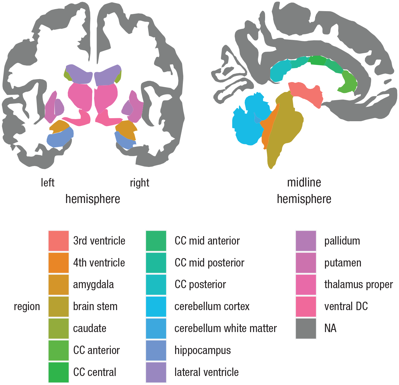
Plotting subcortical atlases using ggseg. Atlases for subcortical structures have some distinct differences from the cortical atlases, such as the Desikan-Killiany atlas (Desikan et al., 2006). For instance, there is no option to show only a single hemisphere. Furthermore, rather than showing lateral and medial surfaces, they show axial, coronal, or sagittal slices. To produce the plot in this figure, the Automatic Segmentation of Subcortical Structures (aseg atlas; Fischl et al., 2002) was supplied to the atlas argument in the ggseg() function with fill mapped to the regions column.

Plotting 3D Mesh Data

Representing brains as 2D polygons is a good solution for fast, efficient, and flexible plotting, and these plots can be easily incorporated in interactive apps such as shiny (Chang, Cheng, Allaire, Xie, & McPherson, 2019). Yet brains are intrinsically 3D, and it can be challenging to recognize the location of a region in a flattened image. This problem is exacerbated in atlases that represent subcortical features because they cannot be flattened into two dimensions, as cortical features can. Hence, we have also provided the ggseg3d package for plotting, viewing, and printing 3D atlases in R. The functionality of ggseg3d is based on tri-surface mesh plots through plotly (Sievert, 2019). The data structure is more complex than that of the ggplot2 polygons, and the package includes additional options, such as for brain inflation, glass brains, and camera locations. Because ggseg3d is based on plotly, the resulting brain atlases are interactive, which is useful for interpretation and public dissemination. We recommend that users familiarize themselves with plotly (Sievert, 2019) before using ggseg3d.

Out of the box, ggseg3d() plots the dk_3d atlas (i.e., a 3D version of the dk atlas; 3D atlases have the same names as polygon atlases but with the added “_3d” suffix) on the LCBC surface (the usual degree of brain inflation used by the Center for Lifespan Changes in Brain and Cognition), but there are two more surfaces available for cortical atlases (Fig. 7). The LCBC surface is a semi-inflated white-matter surface based on the fsaverage5 template subject, a surface template that is included in the ggsegExtra package. All 3D atlases include a colour column that is based on the color scheme used in the source neuroimaging software. The following code starts by loading the ggseg3d library and then plots the default dk_3d atlas in the three available surfaces, as illustrated in Figure 7:

Fig. 7.

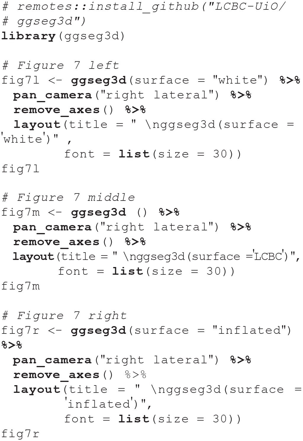
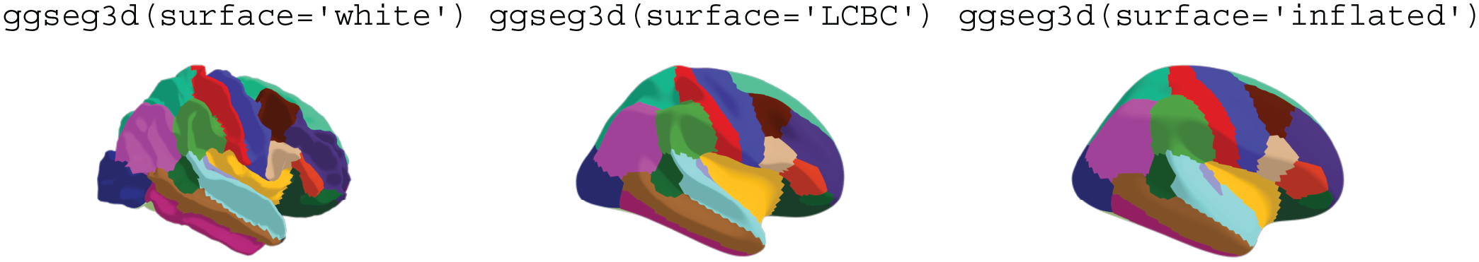
The three surface options provided in ggseg3d atlases. The white surface (left) is the white-matter surface, the LCBC (Center for Lifespan Changes in Brain and Cognition) surface is a semi-inflated (inflated over 10 iterations) white-matter surface (center), and the inflated surface (right) is a fully inflated gray-matter cortical surface provided by the FreeSurfer software. The label above each plot is the literal code used to create it.

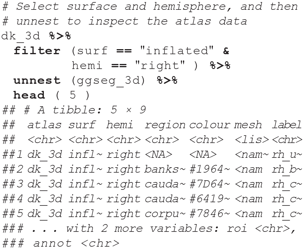
The 3D-atlas data are stored in nested tibbles. Each cortical atlas has data sets for the three different surfaces (see Fig. 7) and the two hemispheres. Only one surface is available for subcortical atlases, as inflation procedures are irrelevant. The ggseg_3d column includes all necessary information for ggseg3d() to create a 3D mesh plot and should not be modified by the user. The additional 3D atlases in ggsegExtra have the same data structure. It is important to note that the coordinates in the plots (X, Y, Z) do not constitute any type of radiological coordinate system, but are arbitrary Cartesian plot coordinates. Although these coordinates are important for running imaging analyses and for reporting of the relative placement of different regions, this information is not currently preserved in ggseg3d. Therefore, information regarding regions’ location in standard radiological spaces (e.g., Montreal Neurological Institute, MNI, space or Talairach space) should be acquired directly from imaging software or documents describing the atlases, not ggseg3d.

Supplying external data

The ggseg3d() function for 3D plots is similar to the ggseg() function for 2D plots; it is used to display some descriptive or inferential statistic by means of a color scale. If the data are not already in the correct long format or do not use naming similar to the naming in the atlas, users should look for a specific surface (and hemisphere, if desired) in the atlas data and then apply unnest(ggseg_3d) to see how the data are organized, as in the following example:

Note the mesh column, which contains lists. Each list corresponds to a region and contains six vectors required to create the mesh of the tri-surface plot of that region. Also note that the label, annot, and region columns could provide matching values for your own data. As in the case of the ggseg()function, the label column should match the region names used in the original neuroimaging software; the region and annot columns provide alternative, or secondary, names. It is thus important to match your regional identifiers with those used in the atlas. To color the segments using a column from the data, a column name from the data needs to be supplied to the colour option, and providing it to the text option will add another line to the plotly hover information.

Customizing colors and the color bar

Custom color palettes can be created either in Hex or in R names. Colors will be evenly spaced in the color scale. A palette may also be supplied as a named numeric vector, in which the vector names are the colors that the user wishes to use and the numeric values are the break points for the colors (e.g., c(“red” = 0, “white” = 0.5, “blue” = 1)). In this way, the user can control the minimum and maximum values of the color scale and also how the gradient is applied. If a color other than the default gray is wanted for the regions not represented in the data, na.colour can be supplied either as a Hex color or as a color name. This option takes only a single color. The following code produces three different color customizations that may be applied in ggseg3d and that are illustrated in Figure 8:

Fig. 8.

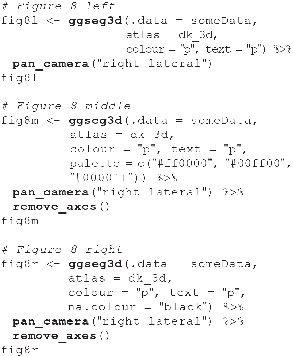
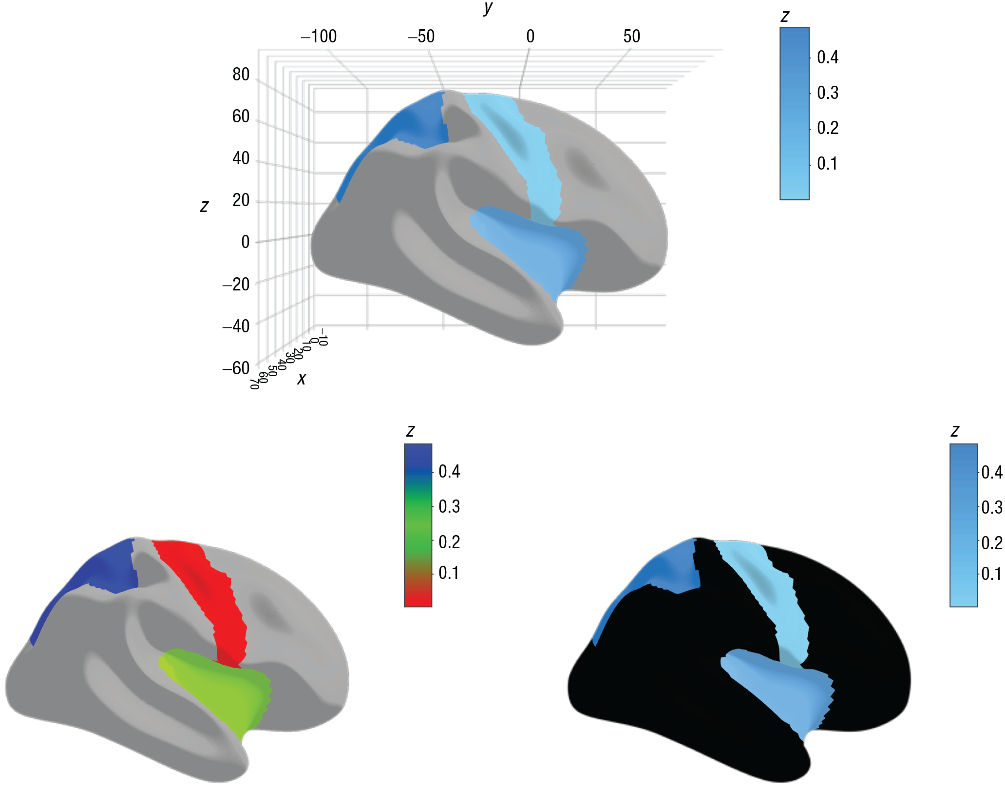
Illustration of the use of color palettes in ggseg3d. Supplying data to ggseg3d() works similarly to supplying data to ggseg(). Because ggseg3d() is based on plotly rather than ggplot2, most aesthetic adaptations must be set in the main function. In the example at the top, we set the parcellation colors with the p column (from the supplied data set) and used the default color scheme for numerical data. The palette argument takes vectors of colors either as Hex codes or as R color names. In the example at the bottom left, Hex codes were used. The color of the NA values (i.e., values not represented in the data) can also be changed through the na.colour argument, as illustrated in the plot at the bottom right, in which the NA values were specified to be black.

Adding a glass brain

A glass brain is a translucent representation of the brain that can provide a frame of reference, particularly in the case of subcortical parcellations, and it serves only as a visual aid. A cortical glass brain can be added to ggseg3d plots through the function add_glassbrain(), which takes three extra arguments: hemisphere, color, and opacity. We recommend using the glass-brain function only when plotting subcortical atlases. The following code shows how you may add a glass brain to a ggseg3d plot of the aseg subcortical atlas (aseg_3d), as illustrated in Figure 9:

Fig. 9.

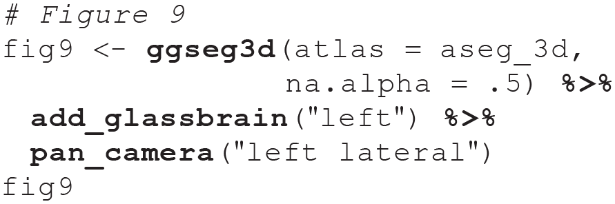
Example of a glass brain added to the visualization of subcortical structure. The plot of the glass brain is controlled by three arguments: opacity, hemisphere, and color. In this example, the glass brain was added for the left hemisphere, and the remaining two arguments were left as their default values. A similar, interactive version of this plot can be found in the online documentation (https://lcbc-uio.github.io/ggseg3d//articles/ggseg3d.html#colours).

More Resources

The ggsed3d() function is based on plotly, and thus additional plotly functionalities can be used to modify and improve the 3D atlas representations. In addition to Sievert’s (2019) online book on data visualization with R, plotly, and shiny, we recommend the following resources: Damiba’s (n.d.-a) examples illustrating how to modify axes in 3D plots and Damiba’s (n.d.-b) basic introduction to tri-surface plots. Finally, we recommend the orca command-line tool (https://github.com/plotly/orca#installation) to save ggseg3d atlas snapshots.

The online documentation for ggseg3d also includes interactive versions of many of the figures in this Tutorial and several more options not covered here (see https://lcbc-uio.github.io/ggseg3d/articles/ggseg3d.html). The online documentation will be updated as new features are required and as we improve user functionality and options.

Additional Atlases

The ggseg and ggseg3d packages have two atlases each: 2D and 3D variations, respectively, of the dk (Desikan et al., 2006) and aseg (Fischl et al., 2002) atlases. These are, however, only two among many meaningful ways of segmenting the brain into different regions. Thus, we have developed the ggsegExtra package, a library with two main functionalities: (a) installing additional data sets from other repositories for plotting with the ggseg and ggseg3d packages and (b) creating custom atlases for ggseg and ggseg3d.

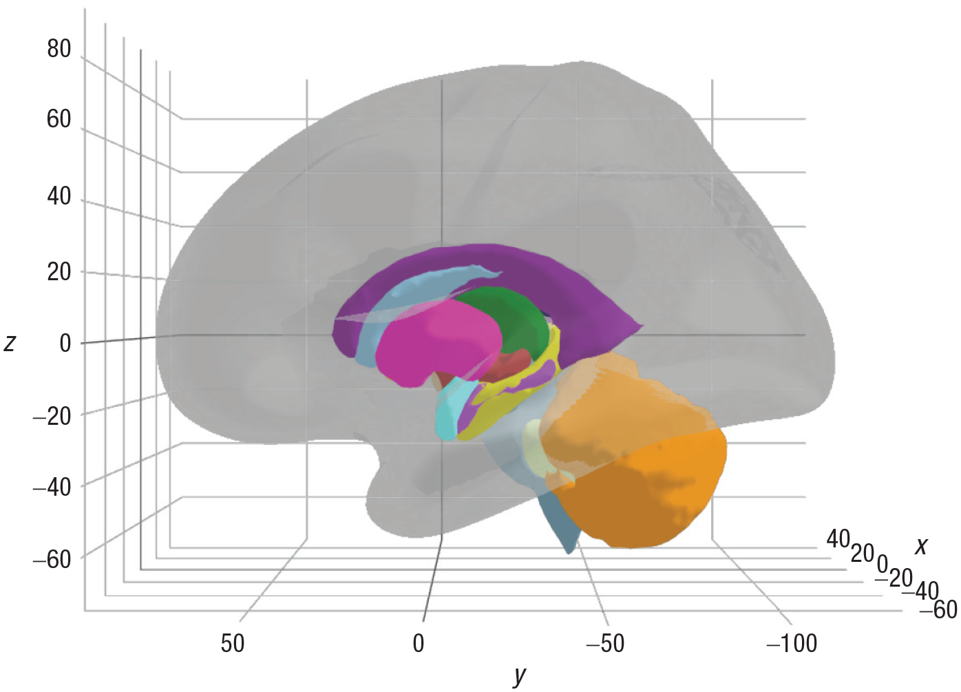
Verified existing atlases

The number of new atlases being created is ever increasing, as research and methods in neuroimaging analysis progress. The ggsegExtra package is intended to be expanded as a community effort, as new and informative atlases are published. A sample of the atlases currently listed in the ggsegExtra package is illustrated in Figure 10 and explored in our shiny demonstration (https://athanasiamo.shinyapps.io/ggsegDemo/). The following code shows how you can look for ggseg-compatible atlases using functions in the ggsegExtra package:

Fig. 10.

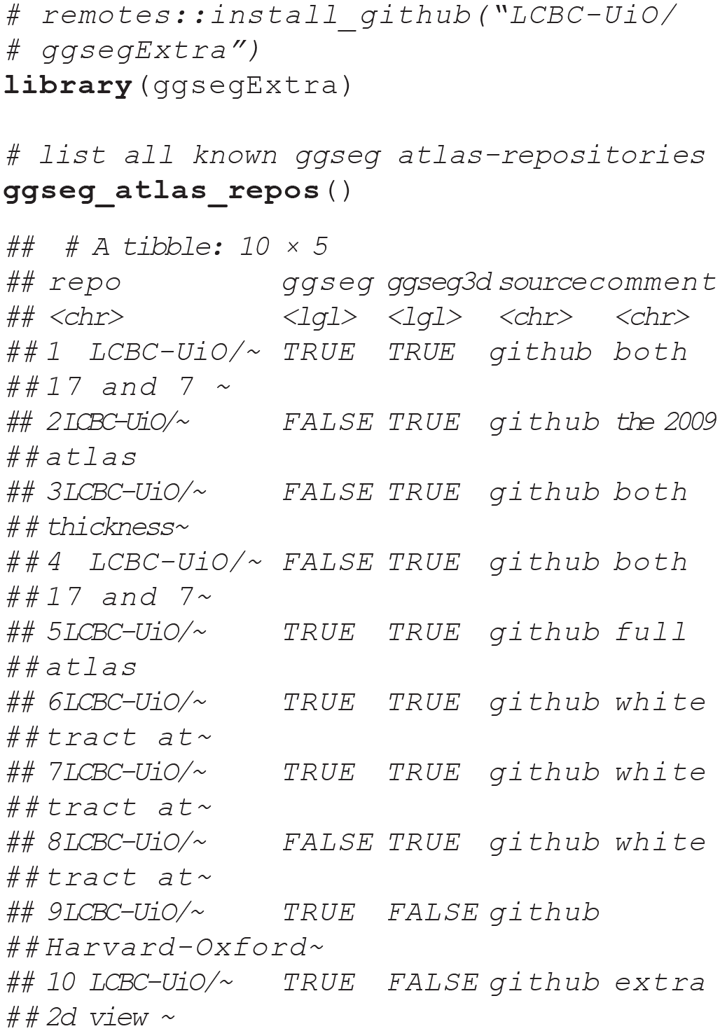
Four example data sets from the ggsegExtra library, plotted with the ggseg() and ggseg3d() functions. The label above each plot is the literal object name for the data set.

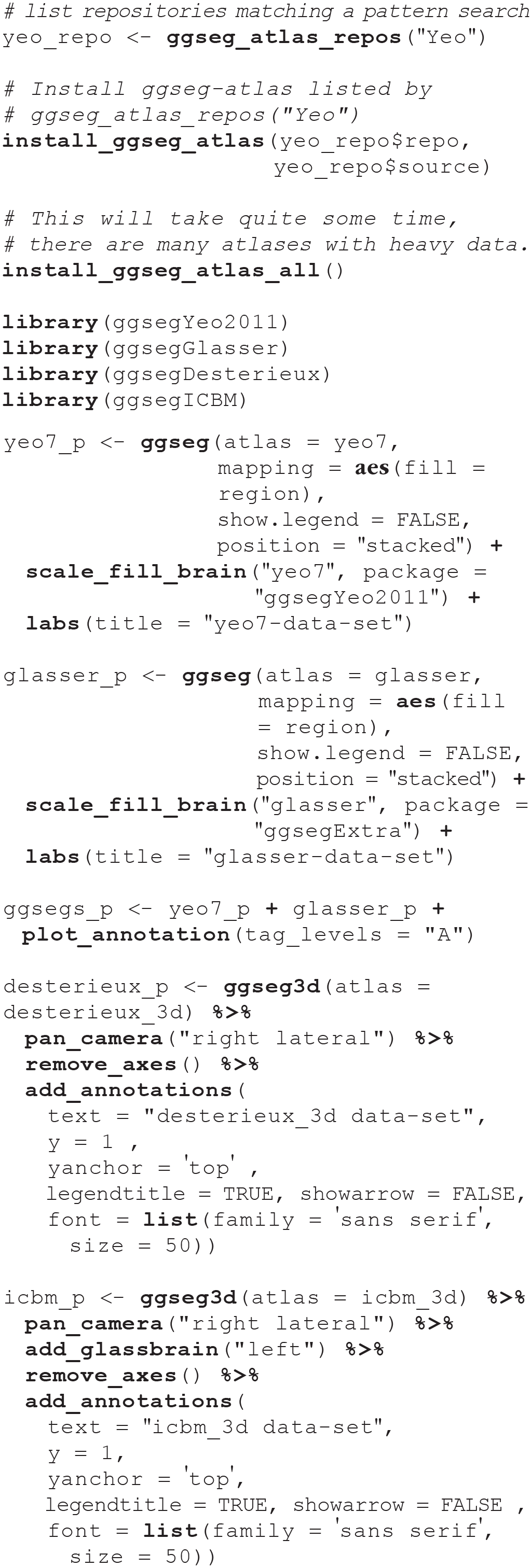
Having identified an atlas you wish to use, you will need to install it as you would an R library. There is a convenience function in ggsegExtra that will help you do that. Alternatively, you can install all the existing atlases. This function will take time to execute and will consume quite some space, as some of the atlases (particularly the ggseg3d atlases) are large. Once the atlases are installed, the atlas packages can be loaded in the same way as any other R package, using the library function. For example, the following code will install and load the atlases illustrated in Figure 10:

Creating custom atlases

In many cases, users would like to create their own atlases based on existing parcellations or their own imaging results. There are several functions in ggsegExtra to aid users in creating atlases compatible with either ggseg or ggseg3d. The procedures depend on the origin of the segmentation (surface based vs. volume based) and what type of system the user is working on. In addition, users need other software dependencies to create new ggseg-compatible atlases. Therefore, we do not describe the procedure here, but refer readers to the “Articles” sections of the online documentation (https://lcbc-uio.github.io/ggsegExtra/index.html) for further explanations and guides. We encourage users who successfully create new atlases to contribute to the ggsegExtra brain-atlas repository by adding the repositories containing their brain atlases to the repository list.

Discussion

The main aim of the ggseg, ggseg3d, and ggsegExtra packages is to ease and streamline visualization of brain-atlas data in R, by gathering a collection of atlases from several scientific sources and providing customized plotting functions. In this Tutorial, we have introduced the packages by presenting some use examples and highlighting the main functions and options that are available. As visualization tools, these packages add complementary functionality to other packages, such as ggBrain (Fisher, 2019) and ggneuro (Muschelli, 2017) in R and software-specific image viewers such as FSLeyes (McCarthy, 2019) and Freeview (Dale et al., 1999). We do not aim to compete with software-specific visualizations or advocate for the superiority of the ggseg packages as visualization tools. After all, flattened 2D polygons do not rely on a meaningful brain coordinate system, and the units of information in 3D meshes are limited to the number of parcellations. On the contrary, we believe that ggseg’s niche among visualization tools resides in its simplicity and its ability to be combined with statistical-analysis pipelines. The possibility for the ggseg packages to serve as interactive tools for dissemination and reproducibility purposes when combined with other technologies, such as Binder (Project Jupyter et al., 2018) or shiny (Chang et al., 2019), is an added benefit (for an example, see the Supplementary Material in Vidal-Piñeiro et al., 2019).

The functions in the ggseg packages provide users with the possibility of adapting the plots to their wishes, and also make it possible to create and contribute to the atlas repository in ggsegExtra. The three ggseg packages offer the following main features:

• A collection of 2D-polygon and 3D-mesh brain-parcellation atlases: The atlas data include the necessary coordinates for plotting and include other helpful information for easier user access.

• Functions for visualization: The ggseg() and ggseg3d() functions are flexible and well adapted to their environment and can be combined with any additional argument from ggplot2 and plotly, respectively. The ggseg() function is a wrapper for geom_polygon from ggplot2, and it can be built upon in the same way as any ggplot2 object. The ggseg3d()function is a plotly wrapper for tri-surface mesh plots that prints 3D atlases.

• Complementary features, like color scales, and functions for converting compatible data frames to atlas classes, reading in likely data sources (e.g., FreeSurfer analysis output), and creating new atlases for use with ggseg and ggseg3d.

The foundations of the ggseg packages trace back to the necessity of visualizing and exploring the life-span trajectories of cortical thickness across different brain regions (see the Supplementary Material in Vidal-Piñeiro et al., 2019). That is, ggseg arose from the need to inspect and display brain information over time (i.e., to include a spatial dimension and a time-varying factor) in a way that overcomes the constraints of print journals and classical 2D plots (e.g., bar plots). The current state of science requires researches to share the results of studies in both high detail and an intuitive manner, so as to permit communication to wide audiences and facilitate reproducibility. Hence, we believe these tools conform to the essence of open science and invite users to improve the code, provide examples or tutorials, and contribute to the atlas collection according to their own interest and needs via the public ggseg GitHub repository (https://github.com/LCBC-UiO/ggseg), ggseg3d GitHub repository (https://github.com/LCBC-UiO/ggseg3d), and ggsegExtra GitHub repository (https://github.com/LCBC-UiO/ggsegExtra).

The ggseg packages are based on ggplot2 and plotly, which are only two of several visualization tools in R, in addition to R base plotting. Although the functionality demonstrated here could also be integrated into packages such as lattice (Sarkar, 2020), both ggplot2 and plotly have become established tools in the R community and have extensive online documentation. This makes them great packages to base further extensions and wrappers on.

Finally, although the ggseg packages are limited to brain parcellations, we believe that the structure and functions of the packages can be easily applied to any scientific field that benefits from data being displayed across the spatial dimension. We encourage readers to borrow the package functionalities and adapt them to their respective fields and structures of interest, such as has already been done with the gganatogram package (Maag, 2018).

Planned Package Improvements

For ggseg, we are working on making a proper geom or stat. Although ggseg() works quite nicely as a ggplot wrapper, it introduces some unexpected work for the user, such as having to group data before faceting. A geom or stat would benefit the user as it would behave more like other ggplot2 geoms and there would be fewer new functionalities to learn.

In the case of ggseg3d, we hope to make it possible to color each individual mesh triangle, and thereby provide users with more flexibility in the plotting. This should also improve the speed of ggseg3d(), which currently is quite slow because each parcellation region is loaded into plotly sequentially. Loading the entire brain mesh at once and then coloring mesh triangles would significantly improve the speed of ggseg3d(). When the package is able to color the mesh triangles directly, rather than each parcellation individually, only full brain representations of each surface (rather than each surface of each atlas) will need to be stored, in addition to text data indexing mesh locations. This would considerably reduce package size, including the package sizes of all the atlas repositories.

Conclusion

Visualization is a fundamental aspect of neuroimaging, used to explore and understand data, guide interpretation, and communicate with colleagues and the general audience. In this Tutorial, we have introduced the ggseg packages, tools for visualizing brain statistics through brain-parcellation atlases in R. This visualization tool easily combines with interactive routines as well as with diverse statistical-analysis pipelines. We hope this tool and Tutorial prove useful to neuroscientists and inspire other researchers to apply the functions in a wide variety of fields and structures.