
Abstract
Methods in data visualization have rapidly advanced over the past decade. Although social scientists regularly need to visualize the results of their analyses, they receive little training in how to best design their visualizations. This tutorial is for individuals whose goal is to communicate patterns in data as clearly as possible to other consumers of science and is designed to be accessible to both experienced and relatively new users of R and ggplot2. In this article, we assume some basic statistical and visualization knowledge and focus on how to visualize rather than what to visualize. We distill the science and wisdom of data-visualization expertise from books, blogs, and online forum discussion threads into recommendations for social scientists looking to convey their results to other scientists. Overarching design philosophies and color decisions are discussed before giving specific examples of code in R for visualizing central tendencies, proportions, and relationships between variables.
Advances of the past decade in open-source software, computational power, and data-visualization science have given rise to both improved ways of visualizing data and the tools to do so. Rapid changes in development are always accompanied by some uncertainties. How does one communicate results most effectively? What are best practices? In the present article, we aim to serve as an intermediary between people developing new data visualizations and specializing in visualization practices and social scientists wishing to apply these techniques to best visualize the results of their research.
Accordingly, this tutorial will have three sections. First, we discuss important design philosophies; second, we speak to decisions about interior components of any figure; and finally, we provide specific examples of improved visualizations for common types of results across the social sciences. Throughout, we include labeled R code for didactic purposes and provide example data sets so readers can determine how to structure their data for the accompanying visualization. Code and data are available at https://osf.io/kx4us/.
Guiding Philosophies
This tutorial is for scientific communication. Much of what is discussed below may not apply depending on one’s goals (e.g., aesthetics) or one’s audience (e.g., children, laypersons). In this tutorial, we assume your goal is to communicate patterns in your data as clearly as possible to other consumers of science. Furthermore, we also assume some basic statistical and visualization knowledge (e.g., do not truncate your y-axis) and focus on how to visualize rather than what to visualize in a given situation.
Information richness
The first philosophy is that of richness. Edward Tufte (1983), a pioneer in data visualization, advocated as principles “Tell the truth” and “Show as much data as possible.” Using visualizations to increase information richness speaks to both principles. Anscombe’s quartet (Fig. 1; Anscombe, 1973) is a famous illustration of how descriptive statistics can conceal important features of your data.
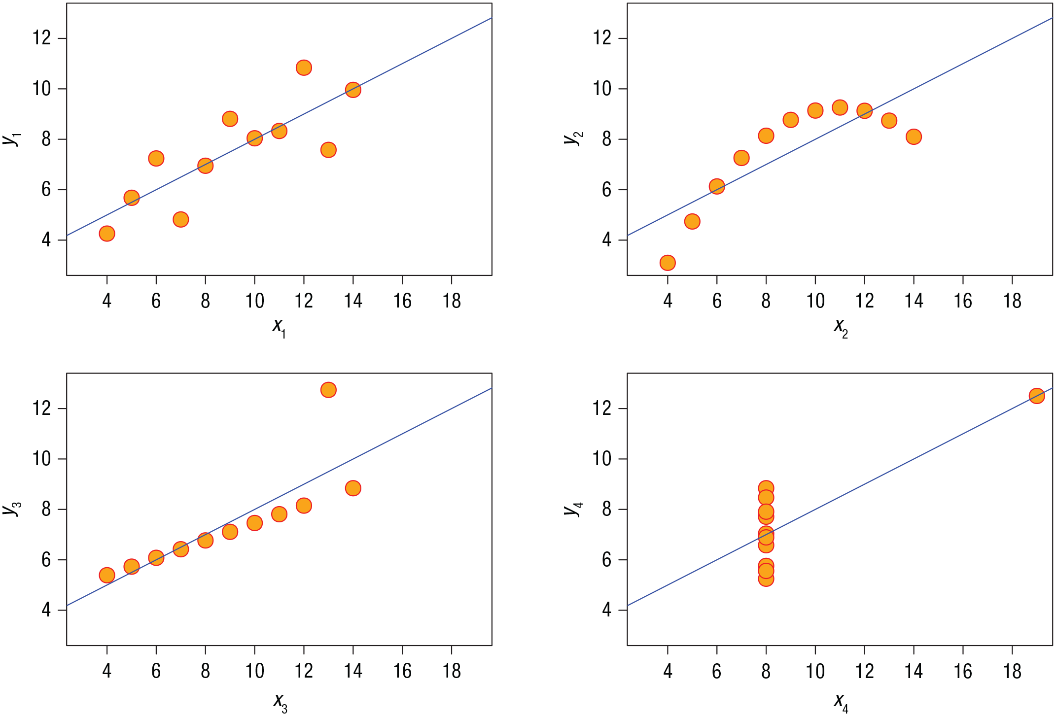
Anscombe’s quartet. In all four data sets depicted, the mean of x is 9, the variance of x is 11, the mean of y is 7.5, the variance of y is 4.12, and the correlation between x and y is .82. Important features of the data are hidden unless the individual observations are visualized.
Every data visualization, like any descriptive statistic, is a simplification of your data. Just like descriptive statistics can mask meaningful underlying variation, basic visualizations that oversimplify your data can do so as well. To the extent that you include more fine-grained information, you can better convey the actual patterns within your data. Consider the classic bar plot: When used to summarize means, bar plots oversimplify because they depict only the means of different conditions, and a great deal of important information is lost (Weissgerber et al., 2015). For example, two conditions might have the exact same mean but very different underlying distributions of observations giving rise to those means (Fig. 2).
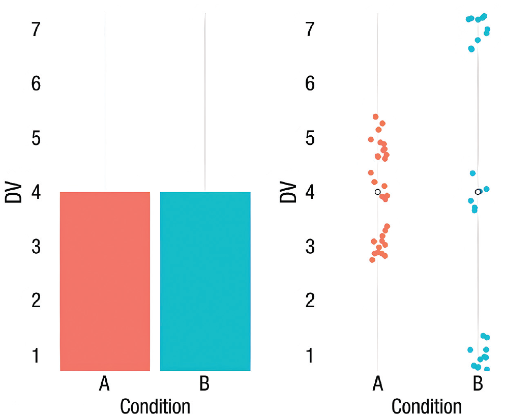
An informationally sparse visualization (left) plotted from toy data. This bar plot reveals two conditions that have identical means. Yet from the same data, plotting the individual observations (right) reveals a very different distribution in each condition giving rise to those means.
Including more visualization features can convey more information to the reader in the same space, thereby increasing the information richness of the visualization. A common first step would involve representing the variability around those means (e.g., error bars). A further step would be representing the distribution of the observations. An additional step would be visualizing the observed data points giving rise to those means and distributions. Readers would then have access to both summary statistics and the variability and shape of the entire distribution of observations, which provide greater understanding of the certainty of any estimate (Helske et al., 2021).
Of course, there is a subjective upper ceiling to how much information can be conveyed in any visualization before it instead hinders understanding. Figure 3 depicts the correlation between attractiveness and intelligence for ratings of targets across four ethnicities (represented by shapes) from participants in 11 world regions (represented by color; with data from Jones et al., 2021). This figure is too rich in information; it hinders the viewer’s comprehension of all the data presented.
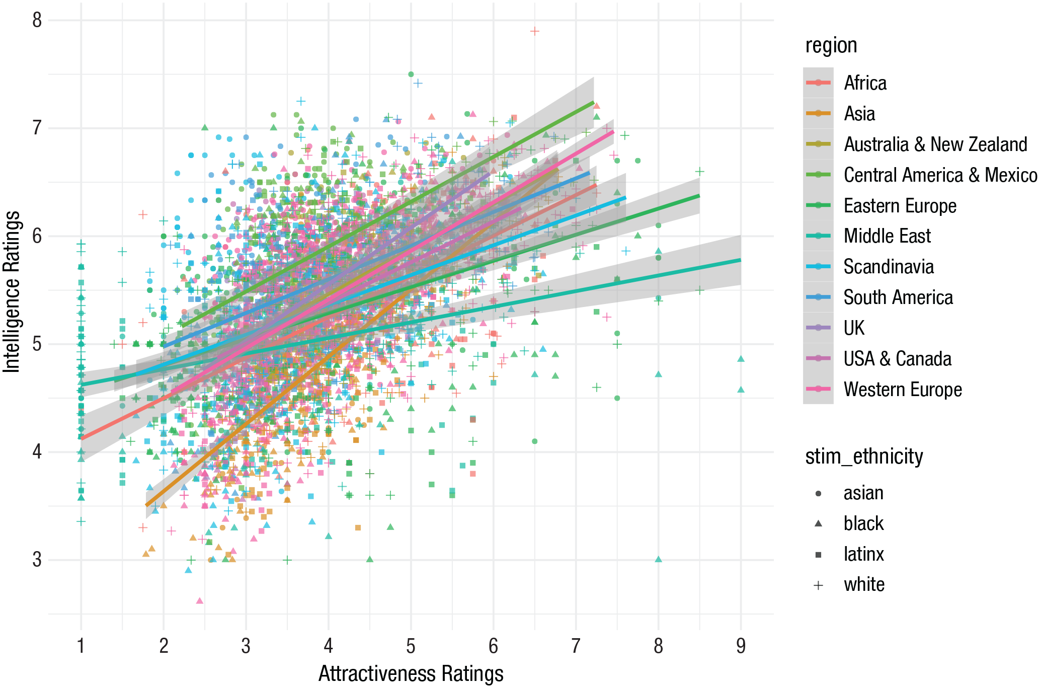
An overinformationally rich visualization. This scatterplot depicts the relationship between ratings of attractiveness and ratings of intelligence made on targets across four ethnicities by perceivers from different world regions.
Overwhelmingly complex figures impede the overarching goal of science communication: to convey information clearly. And deciding when a figure is too rich is unavoidably subjective. Yet as we discuss below, research into the amount of information understood from visualizations can inform exactly where the information richness ceiling might be, depending on the type of visual (Cleveland & McGill, 1985; Heer & Bostock, 2010).
Minimalism
A second important philosophy is that of minimalism. Visualizations can be evaluated in their signal-to-noise ratio, in which signal is the information being conveyed and noise is anything else. The most effective communication maximizes the signal-to-noise ratio by minimizing visual clutter that might interfere with the signal. An extreme version of this argument is that one should justify every single pixel in the visualization. Features not conveying information or allowing readers to assess the patterns more easily should be removed. These might be overlooked features included as default or commonly seen in some software packages (e.g., excessive gridlines in the plot panel). As an extreme example, the serifs in various typefaces are unnecessary pixels because they are not providing additional information. Sans-serif typefaces are more consistent with minimalism. Furthermore, it is rare that any analysis done by most social scientists requires a three-dimensional visualization because it distorts the data and hampers readers’ understanding (Wilke, 2019). Shadows or reflections under text or borders on shapes are all visual noise that is not conveying additional information. To be consistent with the philosophy of minimalism in effective scientific communication, these unnecessary flourishes should be removed.
Color
One of the most important considerations in any modern visualization is that of color. There are a number of concerns to simultaneously navigate when considering your choice of color. The first is inclusivity. Five percent of the human population, 8% to 10% of men, have some sort of color blindness; the most common is red-green color blindness (Neitz & Neitz, 2011). Another concern is that although screen-based reading of articles is now more common, ideally your color choices would still effectively convey information when printed in gray scale because your article will likely be sometimes read in that way. Most importantly, consider the type of information being presented. Are your data categorical? Are there two categories or five? Continuous? Is there a zero point in your continuum? The answers to each of these questions should inform your palette choice.
When your data are categorical, your goal is to choose colors that are maximally differentiable within the color space (while simultaneously being safe for color blindness and gray scale). Exactly what these maximally differentiable colors might be depends on how many categories you need to be equally spaced in color. Excellent tools such as ColorBrewer (Brewer et al., 2003) palettes are valuable and available at https://colorbrewer2.org.
When considering a continuous scale, color gradients can bias a reader’s perception of relative quantitative differences. For instance, certain colors, such as yellow, can create apparent divisions in a scale not actually there because of their high luminosity. Some other color transitions can bias readers into believing there is a bigger value change in a certain part of the scale. It is important that the color gradient consistently changes in value from the top to the bottom of the scale identical to the value change of the numbers the colors represent.
Sometimes researchers may wish to visually represent a zero point along a continuous scale, such as from −3 to 3. In this situation, it is informative to have the positive and negative directions be distinct colors that scale as the values become farther from zero. In addition, the zero point may be best represented as no information, which separates the colors chosen for the positive and negative side of the scales (Fig. 4). Some ideal color palettes can again be found for this situation through ColorBrewer (Brewer et al., 2003).
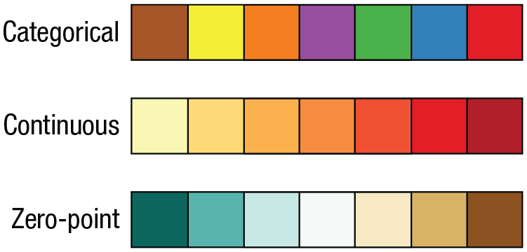
Examples of distinct color palettes for different types of data.
Several packages in R currently represent the state of the art. One is viridis (Garnier et al., 2018). It has been carefully developed to have eight palettes that represent continuous change across a spectrum in palettes that are safe for both color blindness and gray scale (Nuñez et al., 2018). Another is the colorspace package (Zeileis et al., 2019), which is based on human color perception; colors vary along hue, chroma, and luminance dimensions. Likewise, scico (Crameri, 2018) offers gradients that are perceptually uniform and universally readable.
Better Visualization of Common Results
As a general philosophy, goal-centered graph design, or choosing a visualization that highlights your specific hypotheses or goals, will make visualizations most effective. There are some common visualizations that are overwhelmingly used to convey certain types of information. Many of these enjoy their level of popularity because of historic precedent in that area of research and perhaps at one time did comprise the cutting edge of visualization. Yet like any technology, other improved methods have been developed that are now objectively superior. Summarizing these advances very generally, the improvements in visualization hinge on providing improved methods of conveying two types of information (that are related): representations of variance around a central tendency and representations of the overall distribution of the data. In this section, we discuss three common types of information to be conveyed by studies in the social sciences and the modern best practices for conveying that information in data visualizations.
R code and example data are provided in each section. All plots were created using the ggplot2 package (Wickham, 2011), which is required for the tutorial code to run, along with data hygiene packages such as dplyr (Wickham et al., 2021). In addition, we used the viridis (Garnier et al., 2018) and colorspace (Zeileis et al., 2019) color palette libraries, ggExtra (Attali & Baker, 2019), to add marginal density plots and histograms, and gghalves (Tiedemann, 2020) to create the raincloud plots presented below. For those interested in a primer to R, the tidyverse, or ggplot2, see the For Further Reading section at the end of the article. More information on each package is available in the Supplemental Material available online.
# Required R packages
library(“ggplot2”)  # required to make plots
library(“dplyr”)  # for data wrangling/hygiene
library(“viridis”)  # viridis color palettes
library(“colorspace”)  # colorspace color palettes
library(“ggExtra”)  # to add marginal density plots & histograms
library(“gghalves”)  # required to make raincloud plots
In addition to loading these libraries, we set up a custom minimalism theme to reduce the redundancy in R code across our examples in the article. The R code provided in full is available as supplemental material at https://osf.io/kx4us/.
# create ggplot2 theme
# we will use ggplot′s minimal theme as a base and modify it to be usable across our plots
theme_minimalism <- function (){
theme_minimal() + # ggplot′s minimal theme hides many unnecessary features of plot
theme( # make modifications to the theme
panel.grid.major.y=element_ blank(), # hide major grid for y axis
panel.grid.minor.y=element_ blank(), # hide minor grid for y axis
panel.grid.major.x=element_ blank(), # hide major grid for x axis
panel.grid.minor.x=element_ blank(), # hide minor grid for x axis
text=element_text(size=14), # font aesthetics
axis.text=element_text(size=12),
axis.title=element_text(size=14, face="bold"))
}
Central Tendency
Perhaps the most common information social scientists wish to convey are the central tendencies, usually means, in several different conditions. The most common way of representing this information is the bar plot. As alluded to above, certain variants of bar plots present only the mean, a simplification that occludes much information about the underlying data. Improved bar graphs include error bars representing variation around that mean, albeit still in a simplified fashion.
Another common index of central tendency is that of the median. A data visualization based around the median is the box plot, pioneered by Spear (1952) and enhanced into its current form by Tukey (1977). For a dated visualization, the box plot remains extremely effective in conveying a large amount of information about the underlying data. Yet modern improvements have been made.
The addition of the two additional components mentioned above, the actual observed data points and a visualization of the distribution of those points, can increase information richness. These additions far better convey the underlying data giving rise to the central tendencies.
Raincloud plot
Here, we recommend the raincloud plot over alternatives because it best operationalizes the philosophies laid out above (Allen et al., 2019). Essentially, the raincloud plot includes a representation of the overall distribution of observations, the actual observations, and measures of central tendency. If desired, elements of the box plot could be seamlessly integrated in additional layers such that the median and the range of the quartiles of the distribution are included.
In the following example, we use a raincloud plot to illustrate Québec residents’ views on “Bill 21,” a recent law passed by the government of Québec prohibiting some public-sector employees from wearing religious symbols. We measured the extent to which Québecois believed the bill was implemented to address concerns over specific religious symbols (e.g., hijab, crucifix) on items rated on a Likert scale from 1 to 7 (Fig. 5).
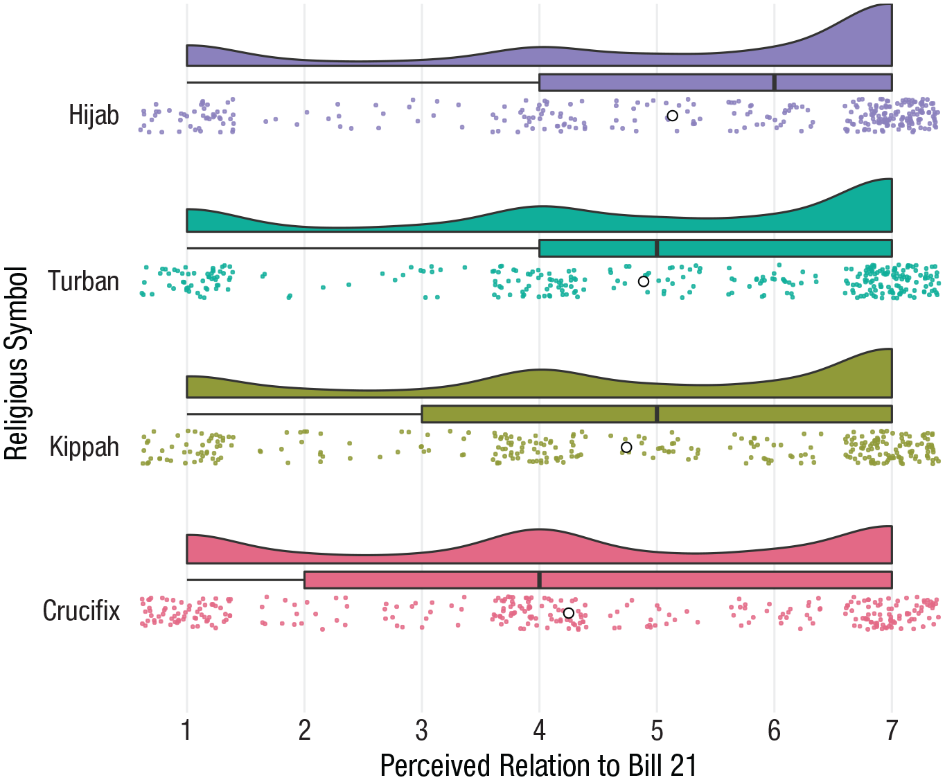
Raincloud plot combining a probability density function, jittered data points, a mean represented by the white circle, and a box plot. The advantage of these additional features is salient here because they reveal several important features of the data, including nonnormal distributions of observations that would be otherwise obscured by presenting only a measure of central tendency like the bar plot.
Some features included above improve the visualization. With large numbers of observations, individual data points overlap. A solution we employed above, on Line 15, is to jitter the location of these data points to reduce this overlap. This slightly changes their location on the x-axis on an irrelevant y-axis so they can be observed. Enhancing this visualization further is the partial transparency of these data points on Line 16 (i.e., α).
 1 # Required packages for raincloud plots
 2 library(“readr”)
 3 library(“gghalves”)
 4
 5 load(“RaincloudData.Rda”)
 6
 7 # Raincloud plot with repeated measurements
 8 f1 <- RaincloudData %>%        # define dataframe
 9  ggplot(aes(x = ReligiousSymbol,   # define x var
10       y = Relation_to_Bill21)) + # define y var
11
12  #Add individual observations to the plot
13  geom_point(
14   aes(color = ReligiousSymbol), # we want different colors for each
   level of x
15   position = position_jitter(width=.1), # add jitter to the observations
16   size=.5, alpha=.8) + # set the size of each dot. alpha adds transparency
17
18  # Define color palette
19
20  scale_color_discrete_qualitative(palette=“Dark 3”) + # add color palette
21  scale_fill_discrete_qualitative(palette=“Dark 3”) + # add fill palette
22
23  # Add the mean for each level of X
24  stat_summary(fun=mean,   # this indicates we want the mean statistic
25         geom=“point”,  # we want the mean to be represented by a geom
26           shape=21,   # use shape 21 (a circle with fill) for the mean
27        size=2, col=“black”, fill=“white”) + # set size, color, &
           fill
28
29  # Add boxplot for observations at each level
30  geom_half_boxplot(aes(fill=ReligiousSymbol), # different colors for
  each level of x
31           side=“r”, outlier.shape=NA, center=TRUE, # styling for
        boxplots
32           position = position_nudge(x=.15),   # position of
      boxplots
33           errorbar.draw=FALSE, width=.2) +    # hide errorbar
34
35  # Add violin plots for observations at each level
36  geom_half_violin(aes(fill=ReligiousSymbol), # different colors for
  each level of x
37          bw=.45, side=“r”,         # styling for the
     violin plot
38          position = position_nudge(x=.3))+ # position of violins
39
40  # Optional styling
41  coord_flip() +             # flip x & y coordinates
42  xlab(“Religious Symbol”) +       # x-axis label
43  ylab(“Perceived Relation to Bill 21”) + # y-axis label
44  scale_y_continuous(breaks=seq(1,7,1)) + # y-axis ticks
45  theme_minimalism() +          # apply our custom minimal theme
46  theme(legend.position=“none”,     # hide legend
47     panel.grid.major.x=element_line())# show major grid for x axis
48 f1
49
50 # save plot
51 ggsave(f1,filename=“figs/Raincloudplot.png”,dpi=300,type=“cairo”,
52    height=14,width=18, units=“cm”)
It is our opinion that these methods of data visualization fully subsume the information conveyed by the bar plot and box plot. In fact, because we do not believe there to be any information present in the bar plot not available in its modern descendants, for representing central tendencies in finalized scientific communication, we think the bar plot should be fully retired.
Cluster heat map
Some researchers may wish to show mean change over time across multiple conditions or categories or as a function of some other continuous variable. When additionally incorporating time, visualizing all the observations and distributions at each point is likely too complex and visually overwhelming. It may be more effective to focus on the information you want to convey most effectively: mean change for multiple categories over time. One visualization ideal for this situation is the cluster heat map (alternatively known as a tile map or level plot; Wilkinson & Friendly, 2009). Here, means over time are represented by color, and each rectangle represents a fixed set of time. This plot enables easy comparison both across many categories and within a category.
In the following example, we use a cluster heat map (Fig. 6) to show how explicit antigay bias changed over time across each state in the United States (with data from Ofosu et al., 2019).
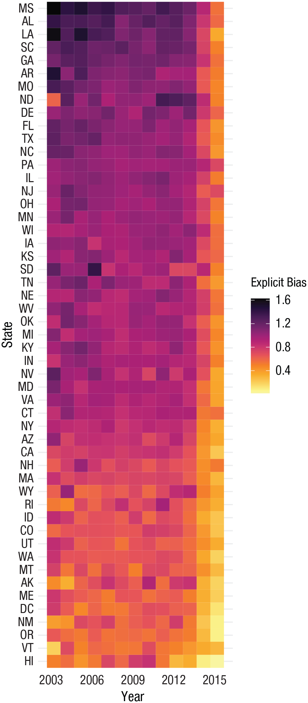
Cluster heat map comparing values of multiple categories over time. Here, the mean values of each state and year are conveyed by color. Although color is not always ideal for presenting values (Cleveland & McGill, 1985), it is an effective option when there is a lot of information to be conveyed because it optimizes information richness. We have sorted this plot by mean prejudice, but it could also be sorted in other ways to enable specific comparisons that emphasize the authors’ points.
In general and for various reasons, we consider the raincloud plot and cluster heat map more consistent with the philosophies laid out above for conveying central tendencies than the bar plot, box plot, violin plot, beeswarm plot, bean plot, pirate plot, lollipop plot, or ridgeline plot, although some of these might still provide some advantages in niche situations.
Proportions or Frequencies
Another common type of information presented is that of proportions or frequencies. Unlike central tendencies, there is no variance to represent around these observed counts. Accordingly, priorities of the data visualization vary. Yet like central tendencies, scientists often wish to visually compare proportions with one another. Because multiple proportions are a percentage of some greater whole, a classic way of representing these data for comparison is a pie chart. We see pie charts (or other circular visualizations) occasionally but less frequently in scientific articles but very commonly in dashboards or scientific communication to the public. However, the pie chart and other circular visualizations have some strong limitations. Research reveals that humans are not very good at perceived circular area and so inaccurately interpret proportions visually represented by a pie chart (Few, 2007; Stevens, 1975). This issue is compounded with multiple pie charts, when readers are comparing proportions not only within a chart but also with other charts (Tufte, 1983). Superior alternatives have been developed.
53 load(“HeatmapData.Rda”)
54
55 # cluster heat map / level plot with change over time in squares
56
57 f2 <- HeatmapData %>%            # define dataframe
58  ggplot(aes(x=Year, y=State, z=Explicit)) + # define x, y, and z
          variables
59
60  # add observations to the heat map
61  geom_tile(aes(fill = Explicit)) + # we will fill the map with colors
         based on
62        # values on the z variable
        (Explicit Bias)
63
64  # Define color palette
65  # For this example, we will use the “Inferno" palette from the
   colorspace package
66  scale_fill_continuous_sequential(palette=“Inferno”,   # define palette
67                  name=“Explicit Bias”) + # name of legend
68  # optional styling
69  scale_x_continuous(breaks=seq(2003,2015,3)) + # x-axis tick marks
70  xlab(“Year”) +                 # x-axis label
71  ylab(“State”) +                # y-axis label
72  ylim(rev(levels(HeatmapData$State))) +     # order y-axis
           alphabetically
73  theme_minimalism() +              # apply our custom
          minimal theme
74  theme(panel.grid.major.y=element_line())    # show major gridline
          for y axis
75 f2
76
77 # we can also order the y-axis another way. below is the code to sort
  the States
78 # by their mean level of prejudice (across all years).
79 yaxisOrder <- HeatmapData %>%
80  group_by(State) %>%
81  dplyr::summarize(avgExplicit = mean(Explicit)) %>%
82  ungroup() %>%
83  arrange(avgExplicit)
84 levels(yaxisOrder$State) <- yaxisOrder$State # this creates the order
          of the states
85
86 # then, we add the following to our figure to sort according to States’
87 # average explicit bias
88 f2 <- f2 +
89  ylim(levels(yaxisOrder$State)) # you may ignore the warning
            that a scale for ‘y’ is
90                 ## already present. This replaces the
       existing scale.
91 f2
92 # save plot
93 ggsave(f2,filename=“figs/levelplot.png”,dpi=300,type=“cairo”,
94    height=23,width=11.5, units=“cm”)    # adjust dims to change
          size of cells
Bar plot
Superior alternatives to pie charts are variants of a bar plot. Although we have critiqued the bar plot for central tendencies, when comparing proportions with one another, a simple bar plot is superior because humans comprehend values represented by length well (Cleveland & McGill, 1985; Heer & Bostock, 2010). Which type of bar plot to choose depends on one’s goals and what one might wish to emphasize to readers (presumably mirroring your statistical comparisons). For example, if you wish to compare one proportion with another, separate columns aligned next to one another far more effectively convey the size of each proportion relative to one another. In Figure 7, we illustrate the proportion of responses on a Likert-type item scaled from 1 to 7 in which greater values represent greater levels of self-reported anti-Black bias made by participants in a single week (with data from Hehman et al., 2018). Because there is no residual, there is no information lost in a bar plot representing proportions or frequencies.
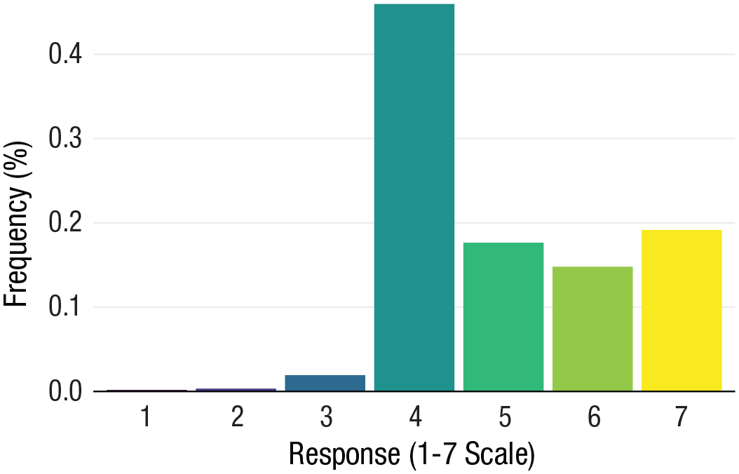
Frequency (%) of responses on a Likert-type item scaled from 1 to 7. Observations were collected at a single time point. Note that even for very small differences, such as Response 1 and Response 2, column length allows for precise comparisons.
Stacked bar plot
For a situation akin to multiple pie charts, when not only comparisons within a cluster are important but also comparing proportions between clusters, stacked bar plots allow for efficient comparison both between bars and within bars. Figure 8 illustrates the changing proportion of responses on the same Likert-type item scaled from 1 to 7 made by participants across 4 weeks.
95 load(“BarandLineplotData.Rda”)
96
97 # bar chart comparing proportions across single category
98 f3 <- BarAndLineplotData %>%   # define dataframe
99  filter(weeks==2) %>%      # filter data only from week 2
100 ggplot(aes(x=response, y=percent, # define x, y variables
101      fill=response)) +   # the fill variable defines the color
        of bars
102 # add bars
103  geom_bar(stat = “identity”, position=“dodge”) + # style of bars. add
           fill=“black” to
104            # set the same color
           across all bars
105 # optional styling
106 # Define color palette
107 # For this example, we will use the “viridis” palette from the viridis
  package
108 scale_fill_viridis(discrete = T, option=“viridis”) +
109 xlab(“Response (1-7 Scale)”) +    # x-axis label
110 ylab(“Frequency (%)”) +     # y-axis label
111 theme_minimalism() +      # apply our custom minimal
          theme
112 theme(legend.position=“none”,    # hide legend
113     panel.grid.major.y=element_line())  # show major grid for
          y axis
114 f3
115 # save plot
116 ggsave(f3,filename=“figs/barplot1.png”,dpi=300,type=“cairo”,
117   height=11,width=16, units=“cm”)
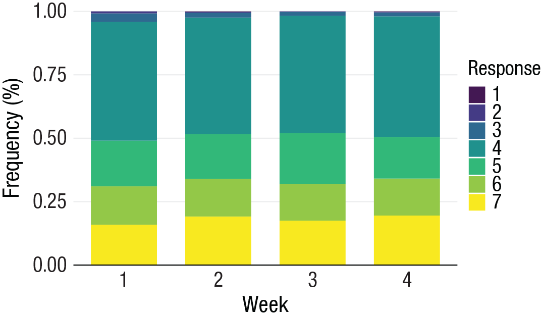
Frequency (%) of responses on a Likert-type item scaled from 1 to 7 in which observations collected across four time points are compared.
Line plot
Like means over time, a common situation is that researchers wish to visualize how proportions change over time or as a function of some other continuous variable. Also like means over time, this is a high amount of information that can become too complex with too many separate stacked bar plots like above. Instead, line plots are an excellent choice.
In the following example, we expand on the bar-plot examples to compare the same proportions across more than 700 time points. Figure 9 illustrates the changing proportion of responses on a Likert-type item scaled from 1 to 7 made by participants across hundreds of weeks.
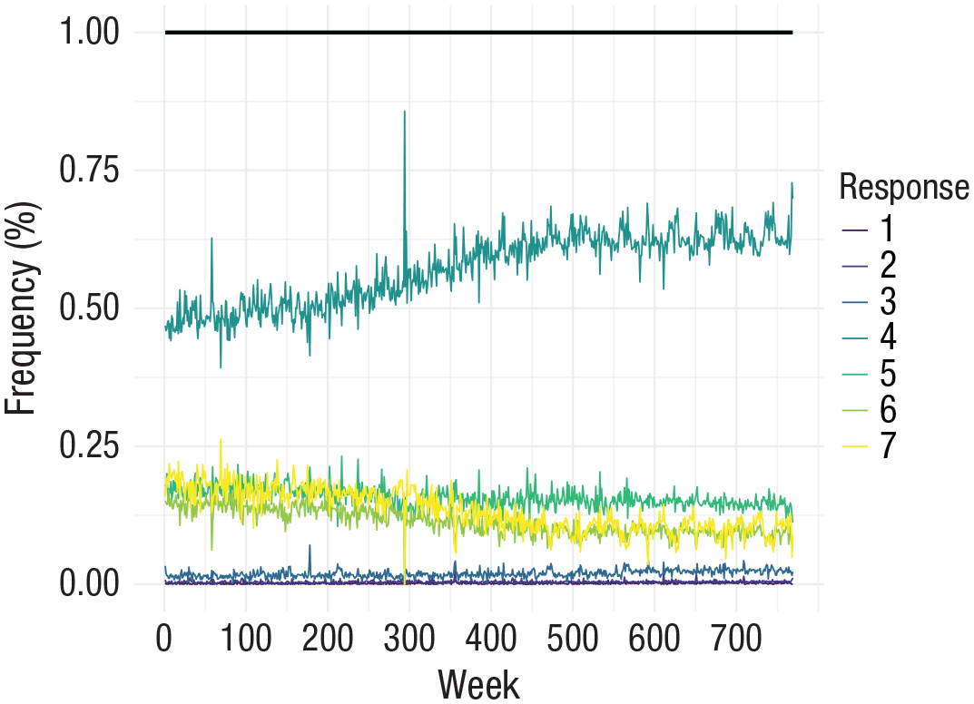
Frequency (%) of responses on a Likert-type item scaled 1 to 7 in which observations collected between 2007 and 2019 are compared. Rather than stacking the values, the lines are plotted over one another so their respective change over time can be compared (in contrast to a stacked area plot, which can impede the accurate perception of values; Few, 2011). We included a black line representing the total per week. The data here are proportions, so this value never deviates from 1. However, when researchers are plotting raw values or frequencies over time, it might be informative to indicate how many total observations occurred per week across all the distinct categories being plotted.
Again, we consider the bar, stacked bar, and line plots more consistent with the philosophies laid out above for proportions than their alternatives, including the pie chart, spider chart, radar chart, tree map, doughnut plot, area chart, stacked area plot, or steam graph, although some of these might still provide some advantages in niche situations.
Relationships
Finally, researchers often want to visualize a relationship between two or more variables, such as a correlation or regression slope. In our subjective opinions, it is for this type of visualization that social scientists have already mostly adopted best practices. We see scatterplots regularly in our respective corner of research. Nonetheless, some additions can improve the information communicated. Like means, it is important here to represent both a central tendency of the relationship and the variance around that relationship. Typically, line graphs are used to represent relationships, and like the other types of information we are covering, they can be improved by better conveying the distribution of data.
118 # bar chart comparing proportions across multiple discrete categories
  (i.e., weeks)
119 load(“BarandLineplotData.Rda”)
120
121 # optional: define custom color palette, assigning a color for each value
122 my.pal <- c(“7” = “#403C91”,
123      “6” = “#8B96D7”,
124      “5” = “#DCEBF9”,
125      “4” = “#F5F5F5”,
126      “3” = “#F2CB89”,
127      “2” = “#F2B552”,
128      “1” = “#FFCB25”)
129
130 # For this example, we want to compare data from weeks 1 to 4
131 # so we will create an index to define which groups to compare
132 index = c(1:4) # compare data from weeks 1 to 4
133
134 f4 <- BarAndLineplotData %>% # define dataframe
135  filter(weeks %in% index) %>% # filter data by weeks variable (weeks 1-4)
136  ggplot(aes(x = weeks, y = percent)) &+   # define x,y variables
137  geom_col(aes(fill = response), width = 0.7)&+ # add bars, set width for bars
138               # the fill variable sets the
                colors
139
140  # optional styling
141  # Define color palette
142  # For this example, we will use the “viridis” palette from the viridis package
143  scale_fill_viridis(discrete=T, option=“viridis”,# color of bars
144        name = “Response”) &+     # change legend title
145  #scale_fill_manual(“Legend”,values = my.pal) &+ # uncomment to use
146                 pre-defined palette
147  xlab(“Week”) &+         # x-axis label
148  ylab(“Frequency (%)”) &+      # y-axis label
149  theme_minimalism() &+       # apply our custom minimal theme
150  theme(panel.grid.major.y=element_line()) # show major grid for y axis
151 f4
152 # save plot
153 ggsave(f4,filename=“figs/barplot2_stacked.png”,dpi=300,type=“cairo”,
154   height=11,width=18, units=“cm”)
155 load(“BarandLineplotData.Rda”)
156 # stacked line plot with total proportion as separate line
157
158 # for this example, we will also add a line to represent the cumulative frequency
159 # calculate cumulative frequency across all levels of x, per y
160 BarAndLineplotData <- BarAndLineplotData %>%
161  group_by(weeks) %>%     # group by week
162  dplyr::mutate(percent_TOTAL := sum(percent, na.rm=TRUE))%>%  # get total % per week
163  ungroup()
164
165 # create stacked line plot
166 f5 <- BarAndLineplotData %>%     # define dataframe
167  ggplot(aes(x = weeks,        # define x variable
168     y = percent,          # define y variable
169      fill = response,      # set grouping variable for bar colors
170     color = response)) &+    # set grouping variable for bar colors
171  geom_line(size = 0.4) &+     # add lines for each group
172
173  # add cumulative frequency to line plot
174  geom_line(aes(x=weeks,y=percent_TOTAL), # add line for total
175     color=“black”, size = 1) &+   # color and size for total line
176
177  # optional styling
178  # define color palette using “viridis” palette from viridis package
179  scale_color_viridis(discrete=T, option=“viridis”,# changes line colors
180         name = “Response”) &+  # legend title
181  xlab(“Week”) &+            # x-axis label
182  ylab(“Frequency (%)”) &+          # y-axis label
183  coord_cartesian(xlim=c(1,769)) &+      # set axis limits
184  scale_x_continuous(breaks=seq(0,769,100)) &+   # x-axis tick marks
185  theme_minimalism() &+          # apply custom minimal theme
186  theme(panel.grid.major.x=element_line(),    # show all major/minor grids
187   panel.grid.major.y=element_line(),
188   panel.grid.minor.x=element_line(),
189   panel.grid.minor.y=element_line())
190 f5
191 # save plot
192 ggsave(f5,filename=“figs/barplot3_lineplot.png”,dpi=300,type=“cairo”,
193    height=13,width=18, units=“cm”)
Improved scatterplot
We consider the scatterplot to be superior to a line plot because it demonstrates both the relationship between variables and the underlying observations that drive that relationship. Including additional features, such as histograms or density plots of the distributions of each individual variable along the x- and y-axes, can further improve the scatterplot. Furthermore, 95% confidence intervals around the estimate of the slope might additionally be included to indicate certainty in the slope estimate that can be hard to glean from the data points themselves.
In Figure 10, we use an improved scatterplot to visualize the relationship between implicitly and explicitly measured anti-Black bias across hundreds of White participants (aggregated to geographic regions from Hehman et al., 2019). We include histograms in the margins of the x-axis and y-axis to show the underlying distributions of each variable.
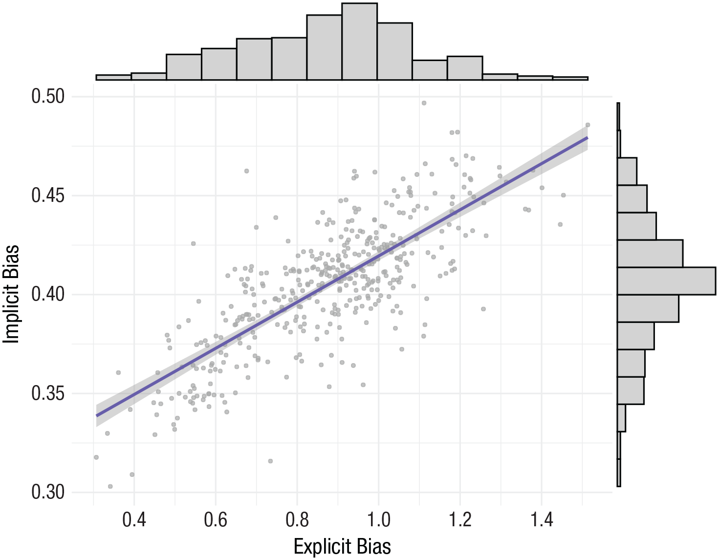
Improved scatterplot visualizing the relationship between implicit and explicit anti-Black bias, including a 95% confidence band of the slope, with histograms of the variable on each axis in the opposite margins.
Contour plot
Sometimes researchers may have so many observations that scatterplots are no longer effective. For instance, with millions of data points, using a scatterplot results in a smear in which no pattern is discernible because of overlap of the points. There are two solutions we prefer in this situation. The first is to randomly sample a percentage of the observations and represent them in the visualization as a scatterplot. However, doing so can require some additional programming. Alternatively, researchers might employ a contour plot, essentially turning the scatterplot into a heat or topographical map in which certain colors represent a higher density of observations (i.e., a modern version of sunflowers; Cleveland & McGill, 1984), which enables readers to still ascertain the underlying relationship while simultaneously seeing the distributions of the observed data across two axes.
To illustrate, in Figure 11, we use a contour plot to represent the same data presented above: the relationship between implicit and explicit anti-Black bias. Rather than the histograms we presented above, here, as a variant, we included density distributions in the margins of the x-axis and y-axis. In fact, we prefer density distributions over histograms because we believe they are more consistent with the principle of minimalism. For consistency, we have used these same data to illustrate this type of visualization. Yet it is important to emphasize we consider contour plots more appropriate when there are more observations (e.g., > 5,000) to ensure a visualization is not too information rich.
194 load(“ScatterPlotData.Rda”)
195
196 # scatterplot
197 f6 <- ScatterplotData %>%         # defines dataframe
198  ggplot(aes(x=ExplicitBias, y=ImplicitBias)) &+  # defines x and y axis variables
199
200  # add observations to scatterplot
201  geom_point(size=1, alpha=.7, color=“darkgray”) &+ # define size and color
202                # alpha adds transparency
203  # add fitted slope and 95% CIs
204  geom_smooth(size=1,method=lm,color=“slateblue”)&+ # define size and color
205                # method=lm indicates linear
                 slope
206
207 # optional styling
208  scale_x_continuous(breaks=seq(0.4,1.6,.2)) &+  # x-axis tick marks
209  scale_y_continuous(breaks=seq(0.3,1.6,.05)) &+ # y-axis tick marks
210  xlab(“Explicit Bias”) &+        # x-axis label
211  ylab(“Implicit Bias”) &+        # y-axis
212  theme_minimalism() &+        # apply custom minimal theme
213  theme(panel.grid.major.x=element_line(),   # show all major/minor grids
214    panel.grid.major.y=element_line(),
215    panel.grid.minor.x=element_line(),
216   panel.grid.minor.y=element_line())
217
218 # add marginal histograms (requires ggExtra package)
219 f6 <- ggMarginal(f6, type=”histogram”,    # add histograms to marginal plot
220        fill = “lightgray”,  # color of histograms
221        xparams = list(bins=15), # n of bins for x variable
222        yparams = list(bins=15)) # n of bins for y variable
223 f6
224 # save plot
225 ggsave(f6,filename=”figs/scatterplot.png”,dpi=300,type=”cairo”,
226   height=14,width=18, units=”cm”)
227 load(“ScatterPlotData.Rda”)
228
229 # contour plot with density plots in the margins
230 f9 <- ScatterplotData %>%          # defines dataframe
231  ggplot(aes(x=ExplicitBias, y=ImplicitBias)) &+ # defines x and y axis
                 variables
232  geom_point(stat=“identity”,size=0.01,alpha=0) &+ # add observations
233  stat_density_2d(aes(fill=..level..),    # add the main contour plot
234      h = 0.1,geom=“polygon”) &+    # change h to adjust
                 binning
235
236  #optional styling
237  scale_fill_viridis(option=“viridis”) &+   # color using viridis palette
238  stat_smooth(method = “lm”, formula = y~x,  # add regression line
239       size=2, color=“black”, se=F) &+ # style of regression line

240  xlab(“Explicit Bias”) &+       # x-axis label
241  ylab(“Implicit Bias”) &+       # y-axis label
242  theme_minimalism() &+          # apply custom minimal theme
243  theme(
244  legend.position = c(0.87, 0.3),    # legend position
245  panel.grid.major.x=element_line(),   # show all major/minor grids
246  panel.grid.major.y=element_line(),
247  panel.grid.minor.x=element_line(),
248  panel.grid.minor.y=element_line())
249
250 # add density plots in the margins (requires ggExtra package)
251 f9 <- ggMarginal(f9, type=”density”)
252 f9
253 # save plot
254 ggsave(f9,filename=”figs/contourplot.png”,dpi=300,type=”cairo”,
255    height=14,width=18, units=”cm”)
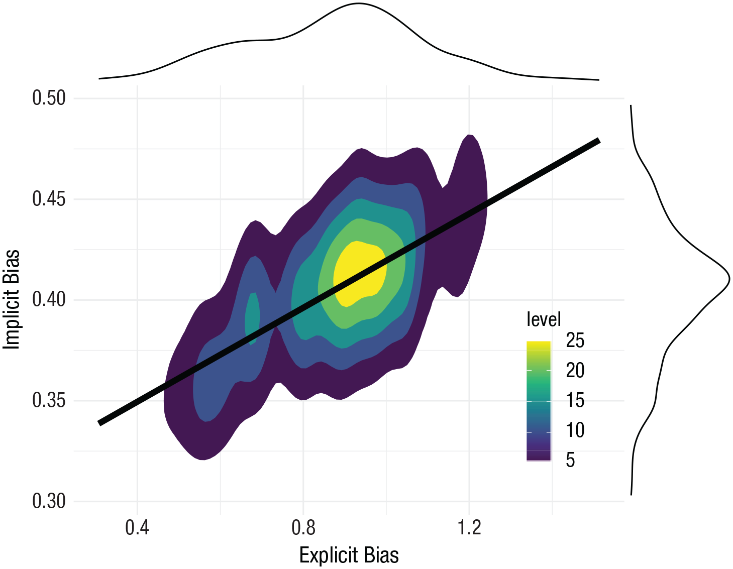
Contour plot visualizing the relationship between implicit and explicit anti-Black bias, with probability density functions in the margins. Areas with higher values on the legend indicate higher density of observations.
Spaghetti plot
Finally, modeling relationships in clustered data in multilevel frameworks is becoming increasingly commonplace. Although showing the grand averaged slope across all clusters is important, it is valuable to show the relationship within each cluster of the multilevel model varying around the grand slope. Effectively capturing this complexity in a single visualization is the spaghetti plot (Fig. 12). We do not recommend including 95% confidence intervals, grid lines, or underlying data points in this plot (as in Fig. 2) because it can become too informationally rich and confusing, depending on the number of clusters. Here, we visualize how attractiveness and intelligence ratings of faces correlate within participants (with data from Xie et al., 2019).
256 load(“SpaghettiPlotData.Rda”)
257
258 # Spaghetti plot for random slopes
259 f7 <- SpaghettiplotData %>%   # define dataframe
260  ggplot(aes(x=attractive,   # define x variable
261     y=intelligent)) &+   # define y variable
262
263  # create random slopes, where each line represents a slope for each cluster
264  # in this example, each cluster is a Participant
265  geom_line(aes(group=ParticipantID, color=ParticipantID), # set clustering
                    variable
266     stat=“smooth”, method=“lm”, # define the line as a linear
              relationship
267     color=“gray”, size=0.8, alpha = 0.5) &+ # define style of lines
268
269  # create a grand slope across all clusters
270  stat_smooth(method=“lm”, formula = y~x,  # grand average slope (linear)
271      color=“coral”,size = 1.5,se=F) &+ # define color, size of
272                average slope line
273
274  # optional styling
275  #scale_color_viridis(discrete=TRUE) &+   # different colors for each
                cluster
276  coord_cartesian(ylim=c(1,7), xlim=c(1,7)) &+ # set axis limits
277  xlab(“Attractiveness Ratings”) &+    # axis labels
278  ylab(“Intelligence Ratings”) &+
279  theme_minimalism() &+        # apply custom minimal theme
280  theme(legend.position=“none”)      # hide legend
281 f7
282 # save plot
283 ggsave(f7,filename=“figs/spaghettiplot.png”,dpi=300,type=“cairo”,
284    height=14,width=18, units=“cm”)
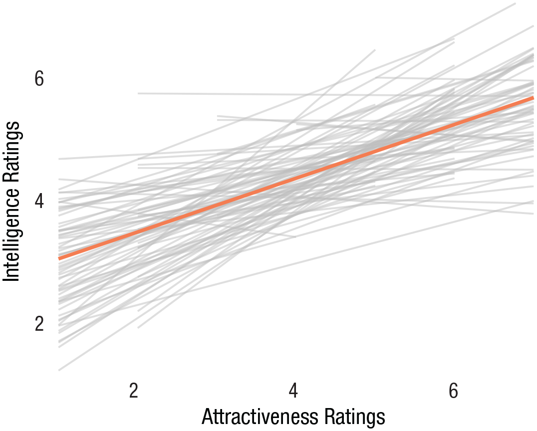
Spaghetti plot visualizing the relationship between ratings of attractiveness and ratings of intelligence made by the same observers evaluating various faces. Thicker coral line represents the grand intercept and slope across all observers. Because of the complexity of the figure, we removed features we would normally include, such as gridlines, observations, or confidence intervals of slopes. In addition, because of the multilevel nature of the data, histograms or density plots on the margins are also inappropriate (because they do not accommodate the clustering within the data).
Recommendations for Further Reading
Although we, the authors, regularly read, think about, and create data visualizations for our research, we are not visualization professionals. Here, we have attempted to distill and present what we consider the information most applicable and useful to other social scientists from people with greater expertise than we. However, we encourage interested readers to seek out the primary sources and modern practitioners and have included a section, For Further Reading, before the Reference section as a starting point.
Summary
Visualizing one’s data effectively to convey information is a science unto itself with research-informed best and worst practices. Yet this is an area in which social scientists receive little training. Here, we aimed to essentially distill advice and information scattered across data-visualization blogs, books, and Internet discussion threads into recommendations viable for individuals communicating their data and results to other consumers of science.
It is not coincidental that our recommendations often hover around the most simple: variants of the bar plot, line plot, or scatterplot. These tried-and-true methods of visualization have persisted across decades because they are effective and clear. Although new visualizations are continually being developed (e.g., beeswarm plot, steam graph), these sometimes have a goal of aestheticism and novelty involved, not clear scientific communication. Although some might envision specific scenarios in which other visualizations are superior, we believe that the recommendations and code we present above will best serve most social scientists in most common situations. We believe it is most important for researchers to keep the guiding philosophies in mind when making their unavoidably subjective decisions about which visualization might be most effective to convey understanding of their data or critical hypothesis test. We hope this tutorial aids in this endeavor.
Recommended Reading
Ismay, C., & Kim, A. Y. (2021). Modern dive: Statistical Inference via Data Science. https://moderndive.com/index.html
A freely and fully available online introduction to R and the tidyverse
Wickham, H., & Grolemund, G. (2017). R for data science. O’Reilly Media. https://r4ds.had.co.nz/
A freely and fully available online introduction to programming in R
Tutorials Point. Learn ggplot2. https://www.tutorialspoint.com/ggplot2/ggplot2_introduction.htm
A freely and fully available online introduction to ggplot2
Wilke, C. O. (2019). Fundamentals of data visualization: A primer on making informative and compelling figures. O’Reilly Media.
An excellent modern resource, with some portions available online, including some code for R.
Tufte, E. R. (1983). The visual display of quantitative information. Graphics Press.
The classic text on data visualization by an initial pioneer in the area
https://www.perceptualedge.com/
A website and blog maintained by data visualization expert Stephen Few, with numerous entries spanning back to 2006
Koponen, J., & Hildén, J. (2019). Data visualization handbook. Aalto korkeakoulusäätiö.
A practical guide to data visualization. For example, see here for comparisons of differential effectiveness of ways of conveying different types of values (e.g., shapes, color, line length, position, etc): “Visual variables,” https://datavizhandbook.info/.
Supplemental Material
sj-docx-1-amp-10.1177_25152459211045334 – Supplemental material for Doing Better Data Visualization
Supplemental material, sj-docx-1-amp-10.1177_25152459211045334 for Doing Better Data Visualization by Eric Hehman and Sally Y. Xie in Advances in Methods and Practices in Psychological Science
Footnotes
Acknowledgements
We thank Neil Hester, Eugene Ofosu, Jennifer Suliteanu, and Chevieve Heri for feedback on an early draft.
Transparency
Action Editor: Julia Strand
Editor: Daniel J. Simons
Author Contributions
Conceptualization: E. Hehman. Data curation: all authors. Visualization: all authors. Writing–original draft: E. Hehman. Writing–review and editing: all authors. Both authors approved the final manuscript for submission.
References
Supplementary Material
Please find the following supplemental material available below.
For Open Access articles published under a Creative Commons License, all supplemental material carries the same license as the article it is associated with.
For non-Open Access articles published, all supplemental material carries a non-exclusive license, and permission requests for re-use of supplemental material or any part of supplemental material shall be sent directly to the copyright owner as specified in the copyright notice associated with the article.