Sage Journals: Discover world-class research

Abstract

Despite the widespread and rising popularity of structural equation modeling (SEM) in psychology, there is still much confusion surrounding how to choose an appropriate sample size for SEM. Currently available guidance primarily consists of sample-size rules of thumb that are not backed up by research and power analyses for detecting model misspecification. Missing from most current practices is power analysis for detecting a target effect (e.g., a regression coefficient between latent variables). In this article, we (a) distinguish power to detect model misspecification from power to detect a target effect, (b) report the results of a simulation study on power to detect a target regression coefficient in a three-predictor latent regression model, and (c) introduce a user-friendly Shiny app, pwrSEM, for conducting power analysis for detecting target effects in structural equation models.

Keywords

power analysis structural equation modeling simulation latent variables open materials

Structural equation modeling (SEM) is increasingly popular as a tool to model multivariate relations and to test psychological theories (e.g., Bagozzi, 1980; Hershberger, 2003; MacCallum & Austin, 2000). Despite this popularity, there remains a great deal of confusion about how to design an SEM study to be adequately powered. Empirical articles reporting SEM analyses rarely describe how sample sizes were determined, so it is unclear to what extent researchers consider sample-size planning in SEM (Jackson et al., 2009). When researchers do report a rationale for sample size, they often rely on rules of thumb that recommend either absolute minimum sample sizes (e.g., N = 100 or 200; Boomsma, 1982, 1985) or sample sizes based on model complexity (e.g., n = 5–10 per estimated parameter, according to Bentler & Chou, 1987; n = 3–6 per variable, according to Cattell, 1978). However, these rules of thumb do not always agree with each other, have little empirical support (Jackson, 2003; MacCallum & Austin, 2000; MacCallum et al., 1999), and generalize to only a small range of model types (Marsh et al., 1998).

The difficulty of forming sample-size recommendations reflects in part the flexibility of SEM, which precludes a one-size-fits-all solution, but it also reflects ambiguity about the goals associated with sample-size planning: Researchers often want to have enough power in a study to know both whether their model will describe the data well and whether their model will be able to detect true target effects. In addition, a consideration unrelated to power is that the sample size must be large enough to ensure a stable model (i.e., to ensure that the estimation algorithm will converge on a solution). Yet the minimum sample size for model convergence is different from the minimum required to detect model misspecification, which in turn is different from the minimum required to detect a target effect within the model (Wolf et al., 2013).¹ A single analysis cannot reveal the minimum sample size that will achieve all of these disparate goals. We next explain two types of power that are relevant to SEM.

Power to Detect a Misspecified Model Versus Power to Detect a Target Effect

Two distinct modeling goals in SEM entail two different kinds of power. One goal is to determine how well the model as a whole describes the data; this goal requires that an analysis has enough power to detect a meaningful level of model misspecification. Another goal is to determine whether there is evidence for specific effects within the model—for example, whether one latent variable predicts another; this goal requires that an analysis has enough power to detect a minimally interesting effect size corresponding to a particular model parameter (Hancock & French, 2013; Kaplan, 1995; Lai & Kelley, 2011). These two types of power may require very different sample sizes, such that an SEM analysis may be well powered to detect a model misspecification but poorly powered to detect a key effect, or vice versa.

Power to detect misspecification

Power to detect a misspecified model is the probability of correctly rejecting an incorrect model, given a specific degree of population misfit. Any structural equation model with positive degrees of freedom entails a set of hypotheses about the relations among variables that put constraints on the population covariance matrix. Fitting the model to data allows researchers to test the hypothesis that the covariance matrix implied by the model is equivalent to the covariance matrix in the population. The effect size to be detected is the degree of true model misfit, which summarizes the degree of discrepancy between the model-implied and population covariance matrices. Thus, the model-misfit effect size does not refer to any particular effect of interest within the model; rather, it is a global metric of how well (or rather, how poorly) the model describes the data.

Many methods for power analysis in this context have been developed over the years. These methods include Satorra and Saris’s (1985) chi-square likelihood-ratio test comparing exact fit of an incorrect null model with that of a correct alternative model (also see Mooijaart, 2003; Yuan & Hayashi, 2003); MacCallum et al.’s (1996) root-mean-square error of approximation (RMSEA) tests of close and not-close fit; and extensions of these tests to other fit indices (e.g., Kim, 2005; MacCallum et al., 2006; MacCallum & Hong, 1997). Several tutorials and online calculators for this type of power analysis are available (e.g., Hancock & Freeman, 2001; Jak et al., 2020; Preacher & Coffman, 2006; Zhang & Yuan, 2018).

Power to detect a target effect

Power to detect a target effect is the probability of correctly rejecting the null hypothesis that a key effect is zero in the population, given a specific true effect size. For example, a researcher might want to know whether latent variable X predicts latent variable Y. In this case, the effect size is the true parameter value (e.g., the size of the regression coefficient). Researchers might find this type of power more familiar and intuitive, because it parallels power for t tests, analyses of variance (ANOVAs), and multiple regressions. Power to detect a target effect uses effect-size metrics that are comparable to those used by power analyses for t tests, ANOVAs, and multiple regressions because these effects can be standardized and converted to common metrics like r and Cohen’s d. Given a true effect of a particular size in the population, power to detect the effect is the probability that the estimated regression coefficient is significantly different from 0.² A target effect in this context can extend beyond structural regression coefficients to any model parameter that can be estimated, such as a factor loading, mean, or residual covariance. Power analysis for detecting a target effect in SEM can be challenging: Researchers must specify not only the value of the target parameter (i.e., its effect size), but also the values of all parameters in the population model. Existing guides require programming knowledge and are either limited to proprietary software (e.g., Mplus; Muthén & Muthén, 2002) or scattered across online resources, posing barriers for researchers interested in conducting power analysis for detecting a target effect in SEM.

We seek to lower those barriers in this article. First, we explain how power to detect a target effect is influenced by features of the model. We demonstrate these explanations with a simulation study and show how power in latent-variable SEM can differ from power in observed-variable regressions. Next, we discuss how to conduct a power analysis for detecting a target effect, and we introduce pwrSEM, a point-and-click Shiny app that allows users to run such power analyses for SEM. We walk readers through the app in a hands-on, example-led guide. Throughout the Tutorial, we offer practical guidance regarding the choices involved in conducting such power analyses.

Factors Affecting Power to Detect a Target Effect

The factors that affect power to detect a target effect in SEM include well-known factors that affect power in any method, such as sample size and effect size, as well as less familiar considerations, such as number of indicators of latent variables, indicator reliability, and the values of other parameters in the model.³ In this section, we briefly review how these factors affect power.

First and most obviously, larger effect sizes lead to greater power. The Wald statistic for testing the null hypothesis that any SEM parameter is zero is the value of the parameter estimate divided by its standard error. As effect size (i.e., the absolute value of the true target parameter) increases, the average estimated value of the parameter increases, which results in larger test statistics on average.

Second, having more information leads to greater power because it increases the efficiency of parameter estimation. Efficiency relates to the variability of the parameter estimate across repeated samples: Smaller sampling variability means that a parameter is more precisely estimated, so it will have (on average) a smaller estimated standard error and confidence interval, and thus a test to detect its difference from zero will be more powerful. The most straightforward way to increase information is to have a larger sample size. Other factors that affect efficiency include completeness of the data (a greater number of missing values means less information and results in larger standard errors and lower power) and distribution of the data (e.g., data that are not multivariate normally distributed, such as ordinal variables and variables with high multivariate kurtosis, also lead to less efficient estimation; Savalei, 2014).

Third, power to detect parameters of a structural model (e.g., latent regression coefficients) is influenced by features of the measurement model, particularly the number and reliability of indicators. In the simple case of a model with a single latent predictor and a single latent outcome, power increases as a function of the coefficient of determination (CD; also known as maximal reliability or coefficient H), which can be understood as the proportion of variation in the set of indicators that is explained by the latent variable. Alternatively, it can be viewed as the reliability of an optimally weighted sum score computed from the items (Bollen, 1989; Dolan et al., 2004; Hancock & French, 2013; Penev & Raykov, 2006). The coefficient of determination can be increased by adding more indicators to the measurement model and/or by increasing the reliability of the existing indicators.

Fourth, power to detect nonzero parameters in SEM may be affected by the size of the structural model (i.e., the number of latent variables that are modeled), the values of all the other structural paths, and the number of estimated paths. Although some suggestive evidence exists (e.g., Wolf et al., 2013, showed that power varies as a function of the number of latent variables in confirmatory factor analyses), we do not know of any studies that have systematically examined how estimation efficiency of one parameter is affected by these factors.

Clearly, a large number of factors can influence power to detect a target effect in SEM. Whereas the effects of some of these factors are well understood, there is no easy way to identify a sample-size requirement that guarantees sufficient power for any given parameter in any given model. In this article, we use a simulation study to illustrate how some of these factors come together to affect power to detect a specific target effect in a specific model, before introducing our Shiny app for power analysis.

Disclosures

The data and code for this article are available via OSF at https://osf.io/h8yfk/. The OSF project at this URL contains R code to reproduce the simulation study, results of the simulation study, and source code for the Shiny Web app pwrSEM. The simulation study was conducted in RStudio (Version 1.2.1335; RStudio Team, 2018) and R (Version 3.6.0; R Core Team, 2019) with the R package lavaan (Version 0.6-5; Rosseel, 2012). The pwrSEM app was created in RStudio and R with the R packages lavaan, rhandsontable (Version 0.3.7; Owen, 2018), shiny (Version 1.3.2; Chang et al., 2019), semPlot (Version 1.1.1; Epskamp, 2015), semTools (Version 0.5-1; Jorgensen et al., 2018), and tidyr (Version 0.8.3; Wickham & Henry, 2019). All simulations conducted are reported. Additional Supplemental Material (http://journals.sagepub.com/doi/suppl/10.1177/2515245920918253) contains details of the methods and results of the simulation study and a second tutorial scenario for pwrSEM.

Simulations: Power to Detect a Target Effect

Using simulated data from a simple structural equation model in which a latent variable Y is regressed on three latent predictors, X, W, and Z, we show how power to detect the regression coefficient of Y on X varies as a function of sample size and characteristics of the model.

Method

We generated data from the model depicted in Figure 1, varying the values of the intercorrelations among latent predictors, factor loadings, number of indicators, and latent regression coefficients. For each condition, we simulated 10,000 data sets each for sample sizes ranging from 50 to 1,000 and generated a power curve. Full details of the simulation design and method are reported in the Supplemental Material.

Fig. 1.

Population model used to generate the simulated data (only the model with three indicators per latent factor is shown). Variables shown in circles are latent variables; variables shown in squares are observed indicators. The target parameter for which power was estimated is β_YX. Labeled paths are parameters that were varied in the simulation. Indicator residual variances were set to 1 – λ² such that all observed variables had unit variance. Residual variance of Y was also fixed such that the total variance of Y = 1.

We fitted two models to each generated data set (see Fig. 2). The first was a structural equation model that corresponded to the population generating model. The second was a multiple regression model based on composite scores formed by summing the indicators of each latent factor. For each fitted model, we recorded (a) whether the estimation algorithm successfully converged on a proper set of parameter estimates with standard errors and (b) whether the p value associated with the null hypothesis ( $H_{0} : β_{Y X} = 0$ ) was less than .05.

Fig. 2.

Models fitted to the simulated data. The model at the top is the fitted structural equation model (only the model with three indicators per latent factor is shown), and the model at the bottom is the multiple regression model fitted to composite scores computed as sums of the set of indicators of each latent variable. All paths correspond to freely estimated parameters, except that the (residual) variances of the latent variables were fixed to 1 for purposes of model identification.

Results

First, we examined model convergence rates and found predictable results: Serious convergence problems arose when the number of indicators was small, item reliabilities were low, and sample size was small. Full results are available in the Supplemental Material.

Next, we computed power as the proportion of converged cases in each condition in which the estimated standardized regression coefficient β_YX was significantly different from 0 (α = .05).⁴ Figure 3 displays the results for a single fixed set of values of the nontarget structural path coefficients, when the correlations (ρ) among the latent predictors were .3 and the nontarget regression coefficients β_YW and β_YZ were 0.1 and 0.2, respectively.

Fig. 3.

Simulation results: power as a function of the total sample size (N), for all combinations of population effect size (β_YX; columns), factor loadings (λ; rows), number of indicators per latent factor (p/f), and analysis model (structural equation model [SEM] or composite-score regression).

As expected, power increased with increasing sample size, effect size, item reliability (factor loadings), and scale length (number of indicators). To understand the effects of the measurement-model parameters (i.e., number of indicators and factor loadings) on power, recall that these two factors together determine the coefficient of determination, which in turn affects power. Table 1 gives the coefficient of determination corresponding to each combination of measurement-model parameters. Because the coefficient of determination can be interpreted as the reliability of an optimally weighted sum score of the items, it can be approximated by the reliability of the (unweighted) scale when the items have similar reliability.

Table 1.

Coefficient of Determination Corresponding to Each Combination of Measurement-Model Parameters in the Simulation Study

Factor loading	Number of indicators
Factor loading	3	5	10
.3	.23	.33	.50
.5	.50	.63	.77
.7	.74	.83	.91
.9	.93	.96	.98

When the effect size was small (β_YX = 0.1, leftmost column of Fig. 3), the only conditions to achieve .80 power in the latent-variable SEM analysis were those with five or more highly reliable (λ = .9) items per factor (i.e., when CD ≥ .96) and very large samples (N ≥ 900). At more reasonable levels of scale reliability, power was quite low. For example, with five indicators having factor loadings of .7 (CD = .83), power just reached .50 at N = 650.

When the effect size was moderate (β_YX = 0.3, middle column of Fig. 3), .80 power in the latent-variable SEM analysis was typically attained at reasonably small sample sizes (as small as N = 200 when the CD reached .74 (e.g., when the measurement model contained three indicators with factor loadings of .7 or 10 indicators with factor loadings of .5). With moderate item reliabilities and five items per factor (CD = .63), a sample size of 300 or more was required to attain power of .80. Notably, three or five unreliable indicators (λ = .3, CD ≤ .33) per factor did not produce sufficient power to detect a medium effect size even at our largest sample size (N = 1,000).

When the effect size was large (β_YX = 0.5, rightmost column of Fig. 3), .80 power was attained whenever the CD was at least .5 (i.e., three or more indicators when λ ≥ .5 or 10 indicators when λ = .3) and the sample size was 250 or more.

These findings exemplify the ways in which effect size, sample size, and reliability of the measurement model contribute to power to detect a target effect. Additional figures in the Supplemental Material compare these results with results for different values of the structural parameters, including when the correlations among latent factors were .5 instead of .3 (Fig. S3) and when the nontarget regression coefficients were both 0.3 instead of 0.1 and 0.2 (Fig. S4). As these supplemental figures demonstrate, it is very difficult to extract general principles about the effect of nontarget structural parameters on power. For example, we found that higher values of the nontarget regression coefficients led to lower power in some conditions (e.g., when the target effect size was high and the reliability of the measurement model was low) but higher power in other conditions (e.g., when the target effect size was low and the reliability of the measurement model was high). These findings highlight the importance of conducting a power analysis specific to one’s own model and including plausible values of all parameters.

Finally, a comparison of the dotted and solid lines in Figure 3 reveals a large effect of the analysis method on power: Conducting a multiple regression on observed composite scores instead of conducting latent-variable SEM resulted in greater power to detect the target regression effect (see also Westfall & Yarkoni, 2016). This difference occurred despite the fact that the regression estimates were attenuated because of measurement error: That is, given the same sample size, power to detect a true observed effect in regression was greater than power to detect that same effect in SEM, even though the effect was nominally larger in SEM because of disattenuation. This finding is consistent with research suggesting that regression coefficients between latent variables are estimated with lower precision than regression coefficients between observed variables (Ledgerwood & Shrout, 2011; Savalei, 2019). This difference was especially pronounced when scale reliability was low: For example, with three items and factor loadings of .3 (CD = .23), power to detect a target effect of 0.4 reached over .80 at a sample size of 750 for the composite-score regression analysis, but the same sample size conferred just .14 power for the latent-variable SEM analysis.⁵

Discussion

Our simulations demonstrated how power to detect a true effect of latent variable X on latent variable Y controlling for latent variables W and Z varies as a function of sample size, target effect size, measurement reliability, and the values of other structural-model parameters. The impact of some of these factors (sample size, target effect size, and measurement reliability) is predictable, in the sense that increasing any of these will necessarily increase power. The impact of other structural parameter values appears to be much harder to predict. When all these factors are considered together, it is very difficult to provide general rules of thumb that can meaningfully inform sample-size planning.

These results also demonstrate how power can be affected by the decision to use latent-variable SEM rather than composite-based observed-variable regression. This discrepancy between latent-variable SEM and observed-variable regression highlights the need to conduct power analyses specific to SEM, because a simpler power analysis based on regressions with observed variables may give a very misleading estimate of the sample size that is required to attain sufficient power for SEM with latent variables.

We caution against generalizing the specific numeric relations from these simulations to different structural models. Power is strongly affected not only by the factors that we manipulated in this study, but also by the structure of the model. For example, we conducted simulations with just one latent predictor instead of three (Fig. S5 in the Supplemental Material displays the results) and found higher rates of convergence overall, comparable performance between SEM and composite regression analyses at moderate to high item reliabilities, and greater power overall. Thus, observations from these simulations should not be treated as rules of thumb unless one is interested in exactly these simulated models, with the same parameter values. This lack of generalizability is precisely why it is crucial for researchers to conduct power analyses that are based on their particular models and plausible parameter values. In the next section, we discuss how to conduct power analysis for detecting a target effect in SEM, and we introduce a Shiny Web app that helps researchers do so.

Conducting Power Analysis for Detecting a Target Effect in SEM

Power analysis for detecting a target effect in SEM can be conducted either via analytic calculations or Monte Carlo simulations. The analytic approach, typically used for t tests and multiple regressions and implemented in such software programs as G*Power (Faul et al., 2009), relies on the asymptotic (large-sample) properties of the test statistic to determine its expected distribution in finite samples. If the sampling distribution of the test statistic is known, determining power is simply a matter of computing the proportion of results in that sampling distribution that would lead to rejecting the null hypothesis of a parameter equaling zero. In SEM, this approach gives solutions that are accurate for very large samples but hold only approximately for smaller samples (Lai & Kelley, 2011). With small- to moderate-sized samples, discrepancies between estimated and asymptotic parameter standard errors can lead to analytic power estimates that do not reflect expected power in practice.

Because asymptotic power calculations can be misleading for small samples, we recommend a Monte Carlo simulation approach, in which many random data sets are drawn from a hypothetical true population model to mimic the selection of multiple random samples from the population. Monte Carlo simulations can be used to calculate power for detecting a target effect in SEM with the following steps:

Specify a hypothesized true population model and all of its parameter values;

Generate a large number (e.g., 1,000) of samples of size N from the hypothesized population model;

Fit a structural equation model to each of the generated samples, recording whether the target parameter is significantly different from 0;

Calculate power as the proportion of simulated samples that produce a statistically significant estimate of the parameter of interest.

This approach was popularized by Muthén and Muthén’s (2002) guide on conducting Monte Carlo simulations to determine sample size for SEM studies (see also Hancock & French, 2013). Yet this approach requires that users have access to Mplus ^{(Muthén & Muthén, 2017)} and know how to program simulations using Mplus syntax and commands. To address the limitations of existing resources on power analysis for detecting a target effect in SEM, and to help researchers conduct their own such analyses, we introduce pwrSEM, a new Shiny Web app. This app estimates power by running Monte Carlo simulations based on a model and sample size that the user specifies via a guided, step-by-step point-and-click interface. It accommodates a wide range of structural equation models, requires no experience in conducting simulations, and provides a suite of features that help researchers choose the model features that underlie their power analysis. Users can access pwrSEM online at yilinandrewang.shinyapps.io/pwrSEM/. Alternatively, users can run pwrSEM locally on their computers by downloading the R source-code file at https://osf.io/tcwyd/, opening it in RStudio, and then clicking on the “Run App” link in the top right-hand corner of the R script section of the RStudio window.⁶

A Tutorial on Using pwrSEM

To illustrate how to use pwrSEM, we present a scenario in which a researcher is interested in powering a study to detect an indirect effect in a mediation model. We walk readers through each step of conducting the power analysis and describe the basic layout and functions of pwrSEM, both from the perspective of general users and from the perspective of the researcher. For simplicity’s sake, we assume that the researcher in this scenario has a good sense of the population model and its parameter values. In the Supplemental Material, we consider a more complex scenario in which a researcher is interested in powering a study to detect several paths in a model, discuss some realistic challenges that users might confront when running a power analysis (e.g., specifying reasonable values of parameters, including factor loadings, structural paths, and residual variances), and highlight solutions that pwrSEM offers.

Research scenario

Suppose that a researcher is interested in planning a study to test a simple mediation model. This model contains a predictor X, a dependent variable Y, and a mediator M, each modeled as a latent variable measured by three indicators. The regression coefficients from X to M and from M to Y (controlling for the effect of X on Y) are respectively labeled as a and b paths (see Fig. 4 for a diagram of the model). The researcher would like to power the study to detect a true indirect effect of a × b.

Fig. 4.

Mediation model used in the research scenario. All paths correspond to freely estimated parameters, except that the (residual) variances of the latent variables were fixed to 1 for purposes of model identification.

Using pwrSEM

Upon launching the app, users see the greeting screen (Fig. 5). The left side panel provides a quick “how to” guide on using the app. The main panel on the right is where users run their power analysis, and it is divided into six tabs: “1. Specify Model,” “2. Visualize,” “3. Set Parameter Values,” “4. Estimate Power,” “Help,” and “Resources.” The first four tabs are ordered by the four steps that users take to conduct the power analysis; the “Help” and “Resources” tabs offer additional information that users might find helpful during the process (we discuss these two tabs in detail in the Supplemental Material).

Fig. 5.

Greeting screen of pwrSEM. The box where users enter their analysis model is prefilled with lavaan code of a sample model.

Step 1: Specify model

Users begin by specifying their analysis model. Currently, pwrSEM accepts lavaan syntax (Rosseel, 2012). After specifying a model, users can decide how they would like to set the scale of the latent variables. Selecting the default option will fix (residual) variances of the latent variables to 1 and allow all factor loadings to be freely estimated. Alternatively, users can choose to fix the first factor loading to 1, allowing (residual) variances of latent variables to be freely estimated. Users confirm their model by clicking on “Set Model,” which will bring them to the next step.

In our scenario, the researcher specifies the measurement model (i.e., how latent variables X, M, Y are measured) and the structural paths among the constructs. Because the researcher is primarily interested in the indirect effect a × b, the component a and b paths can be labeled by adding a* and b* in front of the corresponding predictors, then defining a new parameter ab as the product of the two paths (Fig. 6). The researcher accepts the default option of fixing latent variables to unit variances and clicks on “Set Model” to advance to Step 2.

Fig. 6.

Screenshot showing the model specified by the researcher in Step 1 of pwrSEM.

Step 2: Visualize

Upon proceeding to Step 2, users will see a path diagram of the model specified in Step 1 (generated by semPlot; Epskamp, 2015). Following SEM conventions, the diagram represents latent variables as circles, observed variables as squares, and linear regression coefficients as single-headed arrows. Double-headed loops that begin and end at the same variable represent variances (of exogenous variables) or residual variances (of indicators or endogenous variables), double-headed arrows connecting two variables represent covariances, and triangles represent means (of exogenous variables) or intercepts (of indicators or endogenous variables). Fixed parameters (according to the decision in Step 1) are represented with dashed lines, and free parameters are represented with solid lines. Users can fine-tune the diagram with advanced visualization options, including the ability to change whether the measurement model is shown, change the size of shapes that represent observed and latent variables, and rotate the orientation of the diagram. Once users visually confirm their model, they can click on “Proceed” to continue to Step 3; alternatively, they can click on “Back to Step 1” to modify the model.

In our scenario, the researcher visually confirms that the model is correct, then proceeds to Step 3 (Fig. 7).

Fig. 7.

The researcher’s model as visualized in Step 2 of pwrSEM.

Step 3: Set parameter values

In Step 3, a list of all model parameters is automatically generated from the model set in Step 1 and placed in an interactive, editable table. The parameter table lists every model parameter, its user-specified label, its description, and its type. Users are prompted to set values for all population parameters in the “Value” column. Doing so is crucial because power to detect a target effect depends on both the value of the target parameter and the values of other parameters in the model: As illustrated by our simulation study, power to detect a structural parameter of interest depends on the true size of that parameter as well as the number and true sizes of other parameters. Users set parameter values by double-clicking on the “Value” cells in the table and entering their best estimate of the value of each parameter. Note that the simulation procedure takes these estimates to be true population values; that is, it does not correct for the uncertainty of choosing parameter values. It is therefore important that users estimate power for a range of model parameter values to discover the sensitivity of the power estimate to such variation (we provide an example of a sensitivity analysis later in this Tutorial and in the Supplemental Material). The table operates similarly to a table in spreadsheet software (e.g., Excel): For example, users can copy and paste values from a spreadsheet directly into the table or copy the value of a cell to the cells below by dragging the bottom right corner of that first cell. Once all parameter values are set, users can select the target effects for which they would like to conduct power analysis and proceed to Step 4.

In our scenario, the researcher has a good idea of the likely population parameter values in the model and inputs those values into the parameter table. The researcher sets the factor loading of each indicator of X and Y to .70 (corresponding to a scale reliability of .74 for X and Y), the factor loading of each indicator of M to .80 (corresponding to a scale reliability of .84 for M), and the a, b, and c paths to 0.30, 0.20, and 0.10, respectively. On the basis of these values, the researcher calculates and sets the residual variance of each indicator of X to .51, the residual variance of each indicator of M to .36, the residual variance of each indicator of Y to .51, the total variance of X to 1, and the residual variances of M and Y to .91 and .938, respectively (see Fig. 8). Next, the researcher sets the indirect effect of interest (ab) to 0.06 (the product of the a and b paths). Then the researcher checks the box in the “Effect” column that corresponds to the effect of interest and clicks on “Confirm Parameter Values” to proceed to Step 4.

Fig. 8.

Screenshot showing some of the parameter values set by the researcher in Step 3 of pwrSEM (some values have been rounded by the app).

Note that if researchers do not know what values to set for the residual variances, they can enter the factor loadings and regression coefficients in the standardized metric, leave blank all other parameters, and click on “Set Residual Variances for Me.” In this case, pwrSEM will calculate and fill in the values for the residual variances, which will reflect the difference between a total variance of 1 and the variance that is accounted for by the entered model parameters. In the Supplemental Material, we discuss in further detail how the “Help” tab in pwrSEM can help users set parameter values if they do not have a good idea what those values should be.

Step 4: Estimate power

The last step in pwrSEM’s power analysis is to choose a sample size and the number of samples to simulate. Users might initially specify a feasible sample size based on resources, power to detect misspecification, or other considerations. The number of samples to simulate reflects the desired precision of the power estimate, assuming no uncertainty of the population model: A larger number of samples returns a more precise power estimate, but the analysis takes longer to run. We recommend that users start with a relatively small number of samples (e.g., 100) to get a rough estimate of power before confirming it with a higher number. Optionally, users can also set the desired alpha level and simulation seed (to get computationally reproducible results). Once the sample size and number of samples to simulate are set, users can click on “Estimate Power via Simulations” to start running their power analysis. A progress bar will appear at the bottom right corner of the app interface to show how many samples have been completed. Once simulations are complete, a power table and two histograms will appear. (If there are two or more effects of interest, users can select the effect for which histograms will be shown.) The power table shows the estimated power to detect each target effect as the proportion of converged simulated samples with a statistically significant estimate of that effect (“Power”), as well as a number of other outputs that users might find relevant, such as the convergence rate (in the table note). Below the power table, the histograms show the distributions of p values and estimates of the target effect obtained from the simulated samples.

In our scenario, the researcher first runs a power analysis with a sample size of 200 and 100 simulated samples. Results suggest that the study will have .33 power to detect an indirect effect (ab) of 0.06 in the model. The researcher increases the sample size to 460 and reruns the power analysis, which now suggests that the study will have .81 power to detect the target effect. The researcher confirms this result by rerunning the power analysis with 1,000 simulated samples, obtaining a power estimate of around .85 (Figs. 9 and 10).

Fig. 9.

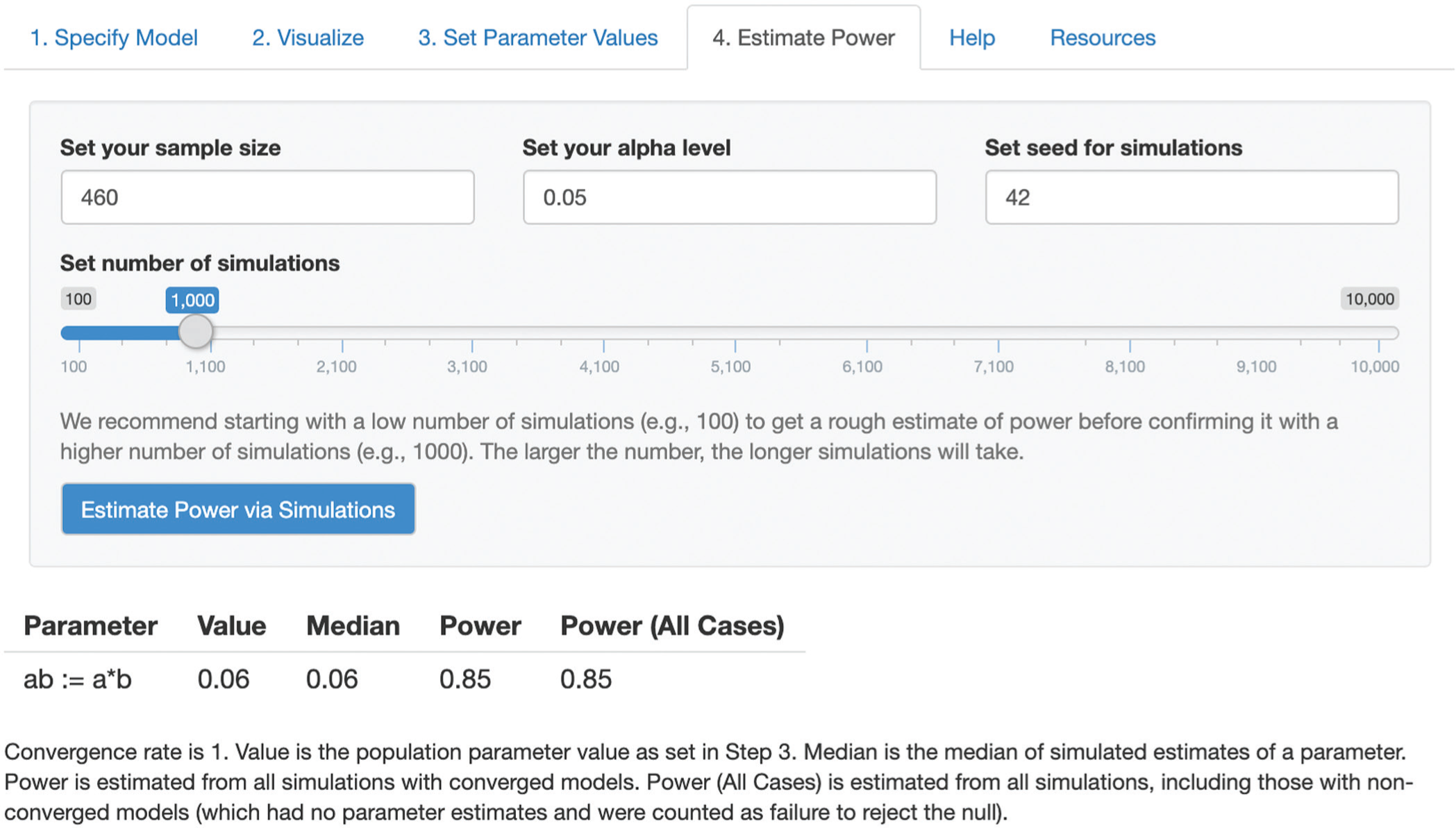
Results of the researcher’s power analysis in Step 4 of pwrSEM.

Fig. 10.

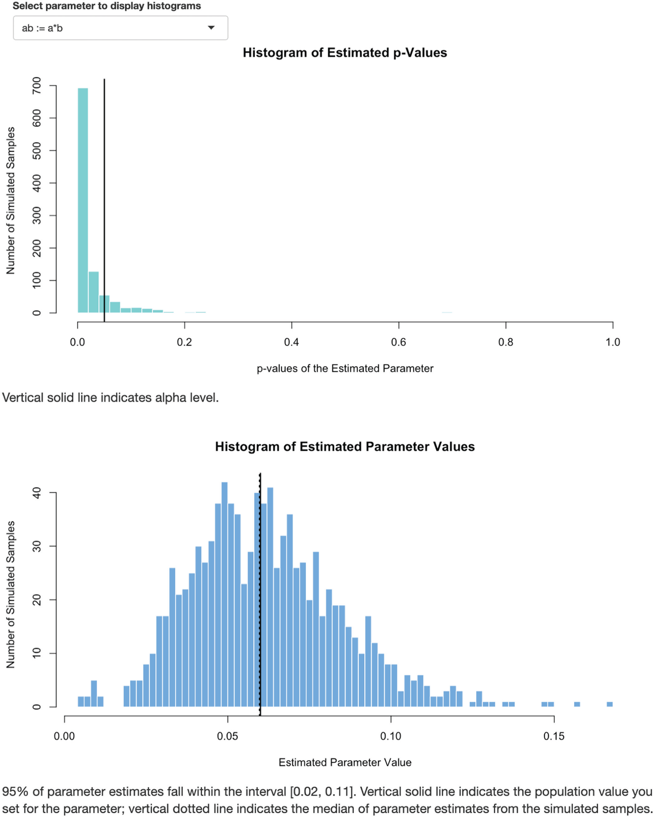
Histograms of the p values and estimates of the target effect in the researcher’s simulated samples.

To explore the sensitivity of this power estimate to specifications of the population parameter values, the researcher reruns the power analysis for detecting the target effect with the sample size of 460 under eight other sets of parameter values, varying both the effect size of b and the factor loadings of M (see Table 2 for details). This sensitivity analysis reveals that varying b and varying λ_M both affect power. The researcher concludes that a sample size of 460 will provide .85 power to detect the indirect effect of interest in the mediation model, but that the power might be lower if the reliability of M is lower or if the size of b (and thus the size of ab) is smaller than specified.

Table 2.

Power as a Function of the Population Value of b and the Factor Loadings of the Mediator (M) in the Example Scenario

λ_M	Power
b = 0.15
.70	.53
.80	.58
.90	.65
b = 0.20
.70	.79
.80	.85
.90	.90
b = 0.25
.70	.95
.80	.98
.90	.98

Note: All power estimates were obtained from power analyses with 1,000 simulations of N = 460. The population model was specified as described in the scenario, except for changes to b (and consequently ab) and λ_M. Residual variances were modified accordingly to maintain unit variances of the latent variables. Scale reliabilities of M were .74 (λ_M = .70), .84 (λ_M = .80), and .93 (λ_M = .90).

Resources

The “Resources” tab of pwrSEM offers additional resources that researchers might find useful. Although this Tutorial and the app focus on power to detect target effects, we emphasize that power to detect model misspecifications is also an important consideration. Thus, we included in pwrSEM an additional calculator that allows researchers to run power analyses for detecting model misspecification using MacCallum et al.’s (1996) RMSEA-based approach. We also provide additional learning resources on SEM for interested users.

Current limitations and potential extensions

We acknowledge that the current version of pwrSEM has a number of limitations. First, to make the app accessible and user-friendly, we assumed that the population model from which the app generates data has the same parameters as the analysis model with which users plan to fit the data. In practice, this might not always be the case (e.g., researchers might intentionally choose an analysis model that is simpler than the population model). Second, because of the computational intensity of fitting structural equation models to a large number of simulated samples, the app currently does not allow for calculation of sample size based on desired level of power. Future work could address this limitation either by using a varying-parameters approach (see Schoemann et al., 2014, 2017) or by solving for N analytically and confirming the value via simulation. Third, the app currently generates only normally distributed data; future work on the app might enable it to accommodate data with other distributional properties, such as categorical data, nonnormal data, and data with a certain amount of missingness. Meanwhile, we encourage researchers interested in these more advanced specifications to implement them in R or other software environments directly.

We remind readers that SEM is a complex statistical technique. Although pwrSEM facilitates power analysis for detecting a target effect in SEM, it assumes that researchers have basic working knowledge of conducting and interpreting SEM. We encourage researchers new to SEM to consult introductory learning resources for SEM (e.g., Kline, 2016; Rosseel, 2020). A list of such learning resources can be found under the “Resources” tab in the app.

Conclusion

Power analysis in SEM can be challenging. This is especially true for power analysis for the purpose of determining power to detect a target effect, which poses technical barriers for many researchers. Consequently, such power discussions remain scarce in the empirical SEM literature, and sample-size planning based on rules of thumb is still common. This consequence is unfortunate in the current era, in which researchers in psychology and many other empirical disciplines are recognizing the problems with underpowered studies and seeking to improve the statistical power of their studies (Begley & Ellis, 2012; Ledgerwood, 2016; McNutt, 2014; Nosek et al., 2012; Nyhan, 2015; Vazire, 2017). Given the popularity of SEM in these disciplines, understanding what power in SEM means and planning research that optimizes it are important steps toward more accurate, reliable findings in the empirical SEM literature.

Of course, it should be emphasized that power is not the only consideration in research design, and sometimes different design considerations may be at odds with each other. For example, our simulation study revealed that power in SEM is strongly affected by item reliability and scale length, but we would not encourage researchers to choose a more reliable but potentially less valid measure of their target construct for the sake of increasing power without considering how such a decision might affect other aspects of the research design. A researcher who replaces an existing measure with a more reliable one might end up inadvertently measuring a narrower or altogether different construct. Not only would doing so compromise construct validity and limit the theoretical usefulness of the measure, but it would also alter the population effect size to be detected (e.g., as in the case of bloated specific factors; Cattell & Tsujioka, 1964). In other words, increasing the reliability of a measure can hurt power if the increase in reliability comes at the cost of validity. Researchers should balance their power goals with other desired ends (e.g., using resources efficiently, achieving estimation accuracy, maintaining procedural fidelity with past research) and tailor research-design decisions to their specific research contexts (Finkel et al., 2015; Ledgerwood, 2019; Maxwell et al., 2008; Miller & Ulrich, 2016; Wang & Eastwick, 2020; Wang et al., 2017).

Yet if researchers take seriously what they learn from their structural equation models, then they need to move beyond rules of thumb, evaluate the power implications of their models, and make planning and inferential decisions accordingly. By illustrating how various factors affect power to detect a target effect in SEM and by introducing a new Shiny app for power analysis, we hope we have provided a resource that will help researchers develop informed understanding of power in SEM and allow them to incorporate power analysis into their empirical research pipeline.

Supplemental Material

sj-pdf-1-amp-10.1177_2515245920918253 – Supplemental material for Power Analysis for Parameter Estimation in Structural Equation Modeling: A Discussion and Tutorial

Supplemental material, sj-pdf-1-amp-10.1177_2515245920918253 for Power Analysis for Parameter Estimation in Structural Equation Modeling: A Discussion and Tutorial by Y. Andre Wang and Mijke Rhemtulla in Advances in Methods and Practices in Psychological Science

Footnotes

Transparency

Action Editor: D. Stephen Lindsay

Editor: Daniel J. Simons

Author Contributions

Y. A. Wang and M. Rhemtulla jointly developed the tutorial concept, designed the simulation study, wrote the data-generation and analysis code, and analyzed and interpreted the data. Y. A. Wang developed the Shiny app. Both authors drafted and edited the manuscript. Both authors approved the final version of the manuscript for submission.

ORCID iDs

Y. Andre Wang

Mijke Rhemtulla

Supplemental Material

Additional supporting information can be found at

Notes

References

Bagozzi

R. P.

(1980). Causal models in marketing. John Wiley & Sons.

Begley

C. G.

Ellis

L. M.

(2012). Raise standards for preclinical cancer research. Nature, 483(7391), 531–533.

Bentler

P. M.

Chou

C. P.

(1987). Practical issues in structural modeling. Sociological Methods & Research, 16(1), 78–117.

Bollen

K. A.

(1989). Structural equations with latent variables. John Wiley & Sons.

Boomsma

(1982). Robustness of LISREL against small sample sizes in factor analysis models. In Jöreskog

K. G.

Wold

(Eds.), Systems under indirect observation: Causality, structure, prediction (Part I, pp. 149–173). Elsevier.

Boomsma

(1985). Nonconvergence, improper solutions, and starting values in LISREL maximum likelihood estimation. Psychometrika, 50(2), 229–242.

Cattell

R. B.

(1978). The scientific use of factor analysis. Plenum Press.

Cattell

R. B.

Tsujioka

(1964). The importance of factor-trueness and validity, versus homogeneity and orthogonality, in test scales. Educational and Psychological Measurement, 24(1), 3–30.

Chang

Cheng

Allaire

J. J.

Xie

McPherson

(2019). shiny: Web application framework for R (Version 1.3.2) [Computer software]. Comprehensive R Archive Network. https://CRAN.R-project.org/package=shiny

10.

Dolan

C. V.

Wicherts

J. M.

Molenaar

P. C. M.

(2004). A note on the relationship between the number of indicators and their reliability in detecting regression coefficients in latent regression analysis. Structural Equation Modeling: A Multidisciplinary Journal, 11(2), 210–216.

11.

Epskamp

(2015). semPlot: Unified visualizations of structural equation models. Structural Equation Modeling: A Multidisciplinary Journal, 22(3), 474–483.

12.

Faul

Erdfelder

Buchner

Lang

A.-G.

(2009). Statistical power analyses using G*Power 3.1: Tests for correlation and regression analyses. Behavior Research Methods, 41(4), 1149–1160.

13.

Finkel

E. J.

Eastwick

P. W.

Reis

H. T.

(2015). Best research practices in psychology: Illustrating epistemological and pragmatic considerations with the case of relationship science. Journal of Personality and Social Psychology, 108(2), 275–297.

14.

Gonzalez

Griffin

(2001). Testing parameters in structural equation modeling: Every “one” matters. Psychological Methods, 6(3), 258–269.

15.

Hancock

G. R.

Freeman

M. J.

(2001). Power and sample size for the root mean square error of approximation test of not close fit in structural equation modeling. Educational and Psychological Measurement, 61(5), 741–758.

16.

Hancock

G. R.

French

B. F.

(2013). Power analysis in structural equation modeling. In Hancock

G. R.

Mueller

R. O.

(Eds.), Structural equation modeling: A second course (2nd ed., pp. 117–159). Information Age.

17.

Hershberger

S. L.

(2003). The growth of structural equation modeling: 1994-2001. Structural Equation Modeling: A Multidisciplinary Journal, 10(1), 35–46.

18.

Jackson

D. L.

(2003). Revisiting sample size and number of parameter estimates: Some support for the N:q hypothesis. Structural Equation Modeling: A Multidisciplinary Journal, 10(1), 128–141.

19.

Jackson

D. L.

Gillaspy

J. A.

Jr. Purc-Stephenson

(2009). Reporting practices in confirmatory factor analysis: An overview and some recommendations. Psychological Methods, 14(1), 6–23.

20.

Jak

Jorgensen

T. D.

Verdam

M. G. E.

Oort

F. J.

Elffers

(2020). Analytical power calculations for structural equation modeling: A tutorial and Shiny app. Behavior Research Methods. Advance online publication. https://doi.org/10.3758/s13428-020-01479-0

21.

Jorgensen

T. D.

Pornprasertmanit

Schoemann

A. M.

Rosseel

(2018). semTools: Useful tools for structural equation modeling (Version 0.5-1) [Computer software]. Comprehensive R Archive Network. https://CRAN.R-project.org/package=semTools

22.

Kaplan

(1995). Statistical power in structural equation modeling. In Hoyle

R. H.

(Ed.), Structural equation modeling: Concepts, issues, and applications (pp. 100–117). SAGE Publications.

23.

Kim

K. H.

(2005). The relation among fit indexes, power, and sample size in structural equation modeling. Structural Equation Modeling: A Multidisciplinary Journal, 12(3), 368–390.

24.

Kline

R. B.

(2016). Principles and practice of structural equation modeling (4th ed.). Guilford Press.

25.

Lai

Kelley

(2011). Accuracy in parameter estimation for targeted effects in structural equation modeling: Sample size planning for narrow confidence intervals. Psychological Methods, 16(2), 127–148.

26.

Ledgerwood

(2016). Introduction to the special section on improving research practices: Thinking deeply across the research cycle. Perspectives on Psychological Science, 11(5), 661–663.

27.

Ledgerwood

(2019). New developments in research methods. In Baumeister

R. F.

Finkel

E. J.

(Eds.), Advanced social psychology (2nd ed., pp. 39–61). Oxford University Press.

28.

Ledgerwood

Shrout

P. E.

(2011). The trade-off between accuracy and precision in latent variable models of mediation processes. Journal of Personality and Social Psychology, 101(6), 1174–1188.

29.

MacCallum

R. C.

Austin

J. T.

(2000). Applications of structural equation modeling in psychological research. Annual Review of Psychology, 51, 201–226.

30.

MacCallum

R. C.

Browne

M. W.

Cai

(2006). Testing differences between nested covariance structure models: Power analysis and null hypotheses. Psychological Methods, 11(1), 19–35.

31.

MacCallum

R. C.

Browne

M. W.

Sugawara

H. M.

(1996). Power analysis and determination of sample size for covariance structure modeling. Psychological Methods, 1(2), 130–149.

32.

MacCallum

R. C.

Hong

(1997). Power analysis in covariance structure modeling using GFI and AGFI. Multivariate Behavioral Research, 32(2), 193–210.

33.

MacCallum

R. C.

Widaman

K. F.

Zhang

Hong

(1999). Sample size in factor analysis. Psychological Methods, 4(1), 84–99.

34.

Marsh

H. W.

Hau

K. T.

Balla

J. R.

Grayson

(1998). Is more ever too much? The number of indicators per factor in confirmatory factor analysis. Multivariate Behavioral Research, 33(2), 181–220.

35.

Maxwell

S. E.

(2000). Sample size and multiple regression analysis. Psychological Methods, 5(4), 434–458.

36.

Maxwell

S. E.

Kelley

Rausch

J. R.

(2008). Sample size planning for statistical power and accuracy in parameter estimation. Annual Review of Psychology, 59, 537–563.

37.

McNutt

(2014). Journals unite for reproducibility. Science, 346(6210), 679.

38.

Miller

Ulrich

(2016). Optimizing research payoff. Perspectives on Psychological Science, 11(5), 664–691.

39.

Mooijaart

(2003). Estimating the statistical power in small samples by empirical distributions. In Yanai

Okada

Shigemasu

Kano

Meulman

J. J.

(Eds.), New de-velopments in psychometrics (pp. 149–156). Springer.

40.

Muthén

L. K.

Muthén

B. O.

(2002). How to use a Monte Carlo study to decide on sample size and determine power. Structural Equation Modeling: A Multidisciplinary Journal, 9(4), 599–620.

41.

Muthén

L. K.

Muthén

B. O.

(2017). Mplus user’s guide (8th ed.). Author.

42.

Nosek

B. A.

Spies

J. R.

Motyl

(2012). Scientific Utopia: II. Restructuring incentives and practices to promote truth over publishability. Perspectives on Psychological Science, 7(6), 615–631.

43.

Nyhan

(2015). Increasing the credibility of political science research: A proposal for journal reforms. PS: Political Science & Politics, 48(S1), 78–83.

44.

Owen

(2018). rhandsontable: Interface to the “Handsontable.js” library (Version 0.3.7) [Computer software]. Comprehensive R Archive Network. https://CRAN.R-project.org/package=rhandsontable

45.

Penev

Raykov

(2006). Maximal reliability and power in covariance structure models. British Journal of Mathematical and Statistical Psychology, 59(1), 75–87.

46.

Preacher

K. J.

Coffman

D. L.

(2006). Computing power and minimum sample size for RMSEA [Computer software]. http://quantpsy.org/

47.

R Core Team. (2019). R: A language and environment for statistical computing (Version 3.6.0) [Computer software]. R Foundation for Statistical Computing. https://cran.r-project.org/bin/windows/base/old/3.6.0/

48.

Rosseel

(2012). lavaan: An R package for structural equation modeling. Journal of Statistical Software, 48(2).

49.

Rosseel

(2020). The lavaan tutorial. Retrieved from http://lavaan.ugent.be/tutorial/

50.

RStudio Team. (2018). RStudio: Integrated development for R (Version 1.2.1335) [Computer software]. RStudio.

51.

Satorra

Saris

W. E.

(1985). Power of the likelihood ratio test in covariance structure analysis. Psychometrika, 50(1), 83–90.

52.

Savalei

(2014). Understanding robust corrections in structural equation modeling. Structural Equation Modeling: A Multidisciplinary Journal, 21(1), 149–160.

53.

Savalei

(2019). A comparison of several approaches for controlling measurement error in small samples. Psychological Methods, 24(3), 352–370.

54.

Schoemann

A. M.

Boulton

A. J.

Short

S. D.

(2017). Determining power and sample size for simple and complex mediation models. Social Psychological and Personality Science, 8(4), 379–386.

55.

Schoemann

A. M.

Miller

P. M.

Pornprasertmanit

(2014). Using Monte Carlo simulations to determine power and sample size for planned missing designs. International Journal of Behavioral Development, 38(5), 471–479.

56.

Vazire

(2017). Quality uncertainty erodes trust in science. Collabra: Psychology, 3(1), Article 1. http://doi.org/10.1525/collabra.74

57.

Wang

Y. A.

Eastwick

P. W.

(2020). Solutions to the problems of incremental validity testing in relationship science. Personal Relationships, 27, 156–175.

58.

Wang

Y. A.

Sparks

Gonzales

J. E.

Hess

Y. D.

Ledgerwood

(2017). Using independent covariates in experimental designs: Quantifying the trade-off between power boost and Type I error inflation. Journal of Experimental Social Psychology, 72, 118–124.

59.

Westfall

Yarkoni

(2016). Statistically controlling for confounding constructs is harder than you think. PLOS ONE, 11(3), Article e0152719. https://doi.org/10.1371/journal.pone.0152719

60.

Wickham

Henry

(2019). tidyr: Easily tidy data with “spread()” and “gather()” functions (Version 0.8.3) [Computer software]. Comprehensive R Archive Network. https://CRAN.R-project.org/package=tidyr

61.

Wolf

E. J.

Harrington

K. M.

Clark

S. L.

Miller

M. W.

(2013). Sample size requirements for structural equation models: An evaluation of power, bias, and solution propriety. Educational and Psychological Measurement, 73(6), 913–934.

62.

Yuan

Hayashi

(2003). Bootstrap approach to inference and power analysis based on three test statistics for covariance structure models. British Journal of Mathematical and Statistical Psychology, 56(1), 93–110.

63.

Zhang

Yuan

K.-H.

(2018). Practical statistical power analysis using Webpower and R. ISDSA Press.

Supplementary Material

Please find the following supplemental material available below.

For Open Access articles published under a Creative Commons License, all supplemental material carries the same license as the article it is associated with.

For non-Open Access articles published, all supplemental material carries a non-exclusive license, and permission requests for re-use of supplemental material or any part of supplemental material shall be sent directly to the copyright owner as specified in the copyright notice associated with the article.

0.00 MB

1.94 MB

1.72 MB