Sage Journals: Discover world-class research

Abstract

Scholars routinely test mediation claims by using some form of measurement-of-mediation analysis whereby outcomes are regressed on treatments and mediators to assess direct and indirect effects. Indeed, it is rare for an issue of any leading journal of social or personality psychology not to include such an analysis. Statisticians have for decades criticized this method on the grounds that it relies on implausible assumptions, but these criticisms have been largely ignored. After presenting examples and simulations that dramatize the weaknesses of the measurement-of-mediation approach, we suggest that scholars instead use an approach that is rooted in experimental design. We propose implicit-mediation analysis, which adds and subtracts features of the treatment in ways that implicate some mediators and not others. We illustrate the approach with examples from recently published articles, explain the differences between the approach and other experimental approaches to mediation, and formalize the assumptions and statistical procedures that allow researchers to learn from experiments that encourage changes in mediators.

Keywords

mediation indirect effects experimental design causal inference open materials

For more than three decades, the most common method of mediation analysis has been measurement of mediation (Baron & Kenny, 1986; MacKinnon, 2008). This method uses regression to demonstrate that the effect of a randomized intervention X on an outcome Y is transmitted through a mediator M. The method is pervasive, especially in social psychology. It is taught almost universally in psychology graduate programs.

Yet as psychologists and statisticians pointed out decades ago, this method is prone to bias (e.g., Judd & Kenny, 1981, p. 607; Robins & Greenland, 1992; Rosenbaum, 1984). In particular, conventional mediation analysis is prone to falsely demonstrating that M mediates the effect of X (Bullock et al., 2010, pp. A3–A4; Glynn, 2012; Rosenbaum, 1984). One of our two aims is to illustrate, with practical examples, how and why the method goes awry.

Our second aim is to offer an alternative method for investigating causal pathways. This alternative is design-based in the sense that it relies primarily on the experimental deployment of treatments that shed light on causal mechanisms. The method is sometimes called implicit-mediation analysis (Gerber & Green, 2012) because it does not rely on path analysis. It consists of two phases: an exploratory phase and a scaling phase. In the exploratory phase, one adds or subtracts ingredients from the assigned treatments to augment or undercut putative mediators. This experimental approach used to be much more common than it is now, which is why articles that advocate a design-based approach to the study of causal mechanisms (Pirlott & MacKinnon, 2016; Spencer et al., 2005) primarily rely on pre-1980s research for examples. In the subsequent scaling phase of implicit-mediation analysis, one uses instrumental variables (IV) regression to examine the effects of mediators on outcomes. Unlike measurement of mediation, the scaling approach does not invite the researcher to estimate both the direct and indirect effects of any kind of intervention on an outcome. Instead, it requires researchers to craft interventions that affect potential mediators while having no direct effect on outcomes; in such cases, IV regression produces an estimate of the intervention’s indirect effect via the proposed mediator or mediators. The robustness of this approach is established by replicating the experiment with various interventions that encourage changes in one or more mediators. A further constraint is that researchers must craft at least one intervention to set in motion each of the posited mediators. In short, there is no free lunch. Repeated attempts to affect suspected mediators in different populations and settings are what allow a researcher to learn about mediation without invoking the strong assumptions of the measurement-of-mediation approach.

To bring our two core arguments to life, we draw on arguments and evidence from a recent article (Gaesser et al., 2020). We choose this article because of the unusual clarity with which it advances and tests its hypotheses about mediation; it also has the virtue of making its data and materials publicly available. Although we are critical of the way in which this article uses measurement of mediation, we think there is much to admire about the way in which the authors reason about mediation, and we believe that their core hypotheses lend themselves to implicit-mediation analysis. Indeed, Gaesser et al. (2020) used something like implicit-mediation analysis themselves in one of their studies, and we elaborate on this point below by using data from one of their studies to illustrate the statistical application of the method.

Our article is organized as follows. We begin with a brief overview of the measurement-of-mediation method popularized by Baron and Kenny (1986), a version of which was implemented by Gaesser et al. (2020). This section of the article calls attention to the strong assumptions that researchers make (often without mentioning or defending them) when employing measurement-of-mediation analysis. When these assumptions are not met, measurement of mediation can produce misleading conclusions about the role played by putative mediators.

We then turn attention to alternative approaches that are rooted in experimental design. Because the most ambitious experimental designs are rarely feasible in psychology, we set our sights on the more realistic goals of implicit mediation and illustrate the method with the running example of “episodic simulation” as used by Gaesser et al. (2020). We close by elaborating on the ways in which implicit mediation differs from other experimental designs that have been proposed for the study of mediation.

Measurement of Mediation

Of the measurement-of-mediation approaches, by far the most widely used is the multi-equation regression method popularized by Baron and Kenny (1986). We break no new ground in this section; instead, our aim is to emphasize that the Baron-Kenny approach, like other approaches rooted in path analysis, depends on assumptions that are difficult to defend. And in practice, authors rarely even try to defend them. For example, of the 55 Journal of Personality and Social Psychology ( JPSP) articles published in 2019 that used measurement-of-mediation analysis, only 14 acknowledged any concerns about the method, and only six attempted to defend its assumptions.¹ (Even in these six articles, the attempted defenses were cursory.) The problem is not limited to JPSP; for example, Vo et al. (2020) found similarly low numbers in their study of mediation analyses that appear in medical journals. To appreciate how strong the underlying assumptions are and why they must be defended on a case-by-case basis, we take a closer look at the statistical model.

Like many other measurement-of-mediation methods, the Baron-Kenny method is based on three regression equations:

\begin{matrix} M_{i} = α_{1} + a X_{i} + e_{i 1} \end{matrix}

(1)

\begin{matrix} Y_{i} = α_{2} + c X_{i} + e_{i 2} \end{matrix}

(2)

\begin{matrix} Y_{i} = α_{3} + b M_{i} + c^{'} X_{i} + e_{i 3} \end{matrix},

(3)

in which i indexes subjects, Y is an outcome of interest, X is a treatment, M is a potential mediator of the treatment’s effect on Y, and e₁, e₂, and e₃ are disturbance terms that represent the cumulative effects of omitted causes. To make credible the claim that X truly affects Y, we assume that X is randomly assigned.

The coefficients a, b, c, and c′ express the causal pathways that link X, M, and Y. The effect of M on Y is b. The total effect of X on Y is c. The direct effect of X on Y is c′. The indirect effect of X on Y that passes through M is ab or, equivalently, c – c′.

We refer to the conventional linear regression estimator of b as $\hat{b}$ . It has long been recognized that $\hat{b}$ may be biased (Glynn, 2012; MacKinnon et al., 2002, p. 100) even when X is randomly assigned (e.g., Judd & Kenny, 1981, p. 607). Specifically, if the sample size were infinite, $\hat{b}$ would converge to

b + \frac{c o v (e_{1}, e_{3})}{v a r (e_{1})},

in which cov(e₁,e₃) is the covariance of e₁ and e₃ and var(e₁) is the variance of e₁ (for a derivation, see Bullock et al., 2010). In other words, even in infinite samples, conventional estimates will equal b plus an additional quantity that depends on the covariance of error terms. Whenever these terms covary, M is confounded: It is not independent of the unobserved causes of Y. Put another way, M is confounded whenever it is affected by an unobserved variable that also affects Y. In such cases, the conventional estimates of b will be misleading. Estimates of the indirect effect, ab, will therefore be misleading as well.² (For definitions of confounded and other terms, see Box 1.)

Box 1.

Glossary

Compliers are subjects whose value of M changes in the expected direction in response to a manipulation X. Stated formally, if X and M are binary, compliers are subjects for whom M_i(X = 1) = 1 and for whom M_i(X = 0) = 0.

Encouragement designs are research designs in which a randomized intervention is used to bring about change in another variable whose effects researchers want to learn. Researchers turn to encouragement designs when this second variable cannot be directly manipulated. In implicit-mediation analysis, a random intervention X is used to encourage change in a mediator M because the aim is to assess whether an X-induced change in M in turn affects Y.

Confounded variables are variables whose values are determined by unobserved factors that also affect the dependent variable. In regression Equation 3, the unobserved factor that affects the dependent variable is e₃. The mediator, M, is confounded if it is determined by e₃, as would be the case if e₁ and e₃ were related.

Exogenous variables are variables whose values are not determined by unobserved factors that affect the dependent variable. Randomized treatments and randomized encouragements are exogenous variables.

Instrumental variables (or instruments) are exogenous variables that meet particular conditions such that they can inform about the average effect of a potentially confounded variable for a subset of subjects known as compliers. See Box 3 for a statement of these conditions. Instrumental variables are relevant to mediation analysis because when they are randomly assigned encouragements, they allow one to estimate mediators’ effects on Y.

To illustrate the conditions under which e₁ and e₃ covary, we look to Experiment 2 in Gaesser et al. (2020). In that experiment, all subjects were presented with a short text that describes a stranger in need: for example, someone who has fallen off a motorcycle. Treatment group subjects were asked to undertake episodic simulation—that is, to imagine helping the person described in the text. Control group subjects were instead asked to critique the style of the text that they have read. The authors found that the episodic-simulation treatment increases subjects’ actual willingness to help. They posited that the treatment is mediated by three factors, and on the basis of a procedure like that of Baron and Kenny (1986), they inferred that one factor—the self-reported vividness with which one imagines helping the stranger—is especially important.³

Why might e₁ and e₃ covary in this study? Any unobserved variable that is causally prior to M and correlated with both M and Y could generate this covariance. In principle, the covariance can be positive or negative, but intuition suggests that it will typically be positive, which implies that unobserved factors move M and Y in the same direction. For example, describing the target of help in the episodic-simulation exercise as a member of an in-group may positively affect both helping-scene vividness and willingness to help (Cikara et al., 2011; Gaesser et al., 2020). These two variables may also be affected by subjects’ egocentrism, their ages (Gaesser et al., 2017; D. C. Rubin & Umanath, 2015), and their intelligence (Guo et al., 2019; Herlitz & Yonker, 2002). We have hardly exhausted the list, and that is an important point. The threat of omitted variables implies that e₁ and e₃ may be highly correlated even if no single omitted variable is strongly correlated with M or Y. In the appendix, we use directed acyclic graphs to illustrate an assortment of scenarios that may give rise to covariance between e₁ and e₃ (see the Supplemental Material available online).⁴

The possibility that cov(e₁,e₃) > 0 implies that estimates that suggest a strong indirect effect are compatible with no actual mediation at all. This possibility is not outlandish: It follows at once from the dependence of $\hat{b}$ on a critical quantity that we cannot observe. Data from Gaesser et al.’s (2020) Experiment 2 illustrate the problem. Of course, the authors’ data and results are consistent with actual mediation under the strong assumptions summarized above. Our point is that they are also consistent with no mediation when these assumptions are relaxed. Consider a simplified version of the authors’ Experiment 2, in which scene vividness is the only mediator under consideration. Using the authors’ data to estimate Equations 1 through 3, we find that $\hat{a}$ = .96 (SE = .01), $\hat{b}$ = .55 (SE = .01), $\hat{c}$ = .49 (SE = .02), and $\hat{c'}$ = −.03 (SE = .02).⁵ This procedure thus suggests “full mediation” by helping-scene vividness: When we control for helping-scene vividness in Equation 3, the estimated direct effect of the treatment is approximately 0. From these results, a researcher would ordinarily declare the exploration of mediators a success: Helping-scene vividness transmits the indirect effect of X to Y, and X seems to have no remaining direct effect on Y.

But this measurement-of-mediation procedure has invoked the assumption that cov(e₁,e₃) = 0. Because the errors are unobservable, the assumption is unsupported and potentially false. The dependence of $\hat{b}$ on this quantity leaves open the possibility that b is actually zero and thus that the indirect effect is actually zero. Indeed, in this example, b will be zero when cov(e₁,e₃) = 1.35 or, equivalently, when corr(e₁,e₃) = 0.53. That is, if corr(e₁,e₃) = 0.53, a standard analysis with the Gaesser et al. (2020) data will produce exactly the results reported in their article—suggesting a large indirect effect—even though the true indirect effect is 0.⁶

In their most general form, the problems that we have discussed are problems of identification. Whenever there is no one-to-one mapping between our data on the one hand and our parameters (the quantities that we are trying to estimate) on the other, the estimates can assume multiple values, even with infinite data. That is, the estimates generated by a statistical procedure depend on the assumptions that one imposes, and in the absence of strong assumptions, such as cov(e₁,e₃) = 0, the parameters of the mediation model may be unidentified. The challenge is easy to see when we consider a simple problem: “I am thinking of two integers that sum to 7. What are they?” The answer is not identified. Conventional mediation analysis is just a more complex form of this type of indeterminacy: Data generated in a world in which M mediates the effect of X on Y may look identical to data generated in a world in which M plays no mediating role whatsoever. Recognition of the challenges of identification is the heart of the design-based approach to mediation analysis that we advocate.

Implicit-Mediation Analysis

Because psychology is largely an experimental discipline, it is natural to think that designing experiments in which the mediator is manipulated is the proper way to address inference problems that arise in the study of mediation. We are certainly sympathetic to this viewpoint, but we are quick to acknowledge the practical constraints that experimental researchers face when they attempt to directly set the values of psychological mediators. Those constraints lead us to propose implicit-mediation designs, which are experimental but more tractable than other proposed experimental approaches to mediation analysis chiefly because they do not require direct manipulation of mediators. We begin this section by describing implicit-mediation designs informally and by illustrating how they may be used in actual studies. We then develop their logic more formally, highlighting their connection to IV regression.

Implicit-mediation analysis consists of two phases: an exploratory phase followed by a “scaling” phase. In the exploratory phase, the experimenter adds or subtracts theoretically relevant ingredients to trigger or restrict mediation pathways. As we explain, the ingredients are “theoretically relevant” because they target the specific pathways that are hypothesized to transmit the effect but not other pathways associated with alternative theories.

The exploratory phase of implicit-mediation analysis is valuable because it may indicate that some variables are plausible mediators and that others are not. But many scholars will want to go further: They will want to quantify the indirect effect that X exerts on Y through M. Even scholars who doubt that effect sizes from lab studies are informative about real-world effect sizes may want this information: For example, they may want to compare the indirect effects that are generated by different lab manipulations. In the scaling phase of implicit mediation, they must come to terms with the assumptions required to get that information. Therefore, we begin by considering the design requirements of the exploratory phase, turning later to the statistical assumptions of the scaling phase.

Exploratory phase: studying the effects of multiple mediators by crafting multiple versions of the treatment

The episodic simulation study aptly illustrates the utility of the implicit-mediation approach. In this case, the first phase of implicit mediation entails testing a series of interventions that would augment or retard the vividness with which participants imagine the person to be helped or the scene in which the incident took place. In many ways, this is what Gaesser et al. (2020) did in their progression of experiments. In Experiment 3, for example, they introduced treatments that involved participants “imagin[ing] themselves positively interacting with the person in the scenario” before the person needs help or “imagin[ing] the person in the scenario as if they were looking at them in a photo with a blank background” (p. 693). These new treatments retain an essential feature of the main treatment: In all cases, the authors were asking subjects to imagine others. But by design, these new treatments do not require subjects to imagine helping others, which the authors posited was essential to generating large effects on willingness to help. Their strategy was to see whether these other forms of “imagined contact,” which were posited to set in motion different mediators, were sufficient to generate as much willingness to help. They found weaker effects of the alternative treatments on their main posited mediator, helping-scene vividness,⁷ and they also found that the alternative treatments created less willingness to help (see Gaesser et al., 2020, Table 3 and Figure 5). This combination of implicit-mediation-style results bolsters the argument that their main treatment works through their posited mediator.

Researchers designing studies with implicit mediation in mind should measure a range of potential mediators, including mediators associated with competing theories. If the competing theories are held to be incorrect, these competing mediators should not be affected by X.⁸ For example, if the claim is that episodic simulation (X) affects helping behavior (Y) only by making the scene more vivid (M), episodic simulation should not also affect other mediators that affect Y, such as participants’ sense of anxiety about intervening to help another person.

Conversely, the mediating role of M is suggested when both M and Y change after different variants of X are deployed.⁹ Is it the case that a wide array of different X-induced changes in M coincide with X-induced changes in Y? If so, that would be strong evidence in favor of the proposition that M affects Y regardless of how changes in M are brought about. To borrow an example from Gerber and Green (2012, Chapter 10), biomedical experts believe that consumption of limes (X) cures scurvy (Y) through the mediator (M) of vitamin C in the bloodstream. The reason that scientists are convinced that vitamin C is the mediating pathway is that any method of increasing vitamin C in the bloodstream—whether the X be a vitamin C tablet, a lime, or a serving of broccoli—suffices to cure scurvy.

More ambiguous are instances in which some X-induced changes in M affect Y and others do not. It may be that M is not in fact a cause of Y and that some X interventions transmit their influence on Y through other mediating channels. Or it may be that whether M affects Y depends on moderating conditions, such as the context or the attributes of the participants. Grappling with these kinds of ambiguities requires a systematic and sustained research effort.

To illustrate the challenges of interpretation, imagine that a researcher is investigating the Gaesser et al. (2020) hypothesis: The effect of episodic simulation (X) on willingness to help (Y) is mediated by the vividness with which people imagine a given scenario (M). Episodic simulation is induced by asking people to imagine and then to write about a scenario in which they help another person. To use implicit-mediation analysis, the researcher might begin by assigning some subjects to write for a long period and assigning others to write for a short period. The researcher would then investigate the effect of this timing manipulation. Suppose that assigning subjects to write for a long period increases scene vividness (M) but fails to change willingness to help (Y). This result suggests that scene vividness may not mediate the Gaesser et al. effect.

But suppose that instead of implementing that manipulation, the researcher changes the original Gaesser et al. (2020) instructions in the baseline treatment group: “Make sure to generate as much detail as possible . . . creating a vivid and elaborate event where you strongly see the scenario in your mind’s eye” (Gaesser et al., 2020 online materials). Some subjects are assigned to receive all of the standard instructions, whereas others receive a version in which the instructions to imagine vividly do not appear. Suppose that this final manipulation affects both the vividness of the imagined scene and subjects’ willingness to help. This implicit-mediation analysis does not tell the researcher with precision about the extent to which the effect is mediated by scene vividness, and the possibility that the manipulation set in motion a mediator that is correlated with but distinct from helping-scene vividness cannot be ruled out. But this result sets the investigator down a fruitful path of further inquiry in which the aim is to show whether different ways of inducing changes in helping-scene vividness also affect willingness to help. Any one study, viewed alone, may mislead us; only by assembling a variety of manipulations can we develop a clear sense of whether M is a mediator. And only by repeating the exercise in different settings and with different subject pools can we develop an empirically grounded sense of for whom and under what conditions M is a mediator.

Although we have focused on Gaesser et al. (2020) to illustrate the ideas of the exploratory phase, those ideas can be applied to a wide range of studies. See Box 2 for other examples.

Box 2.

Applications of the Exploratory Phase of Implicit-Mediation Analysis

The applicability of the exploratory phase of the implicit-mediation approach is hardly limited to work in the style of Gaesser et al. (2020). On the contrary, a large part of the approach’s appeal is its feasibility across many domains. Here are three illustrative examples:

Harmon-Jones et al. (2019) found that “pain offset,” the termination of painful experiences, makes people less prone to ruminate about negative stimuli that they subsequently encounter. To investigate the effect, the authors manipulated the experience of physical pain—for example, pain induced by hand-grip exercises. They examined whether the effect was mediated by “pain-offset relief,” a change in affect that follows the cessation of pain. In their experiments, some subjects were randomly assigned to a painful experience, and after the experience was terminated, all subjects were exposed to a negative stimulus—for example, a sad movie. The hypothesis was that relief (i.e., change in affect) mediates the effect of pain offset, causing subjects who have recently experienced pain to ruminate less over the subsequent negative stimulus (i.e., the sad movie). We depict the hypothesized relations among the variables in a diagram on page A9 of the Supplemental Material available online.

An implicit-mediation approach to this hypothesis entails crafting treatments that vary the level of relief that subjects experience after the cessation of pain. For example, some subjects might be exposed to more intense pain than others, which would lead to greater feelings of relief when the pain ceases. If relief is truly a mediator, one should observe less rumination among these subjects than among others. (The authors suggested this manipulation at the end of their article.) Alternatively, pain might cease in ways that do not increase positive affect or reduce negative affect. For example, subjects may be assigned to experience pain offset in the aftermath of a physical competition with a confederate. Physical activity would be held constant in these conditions, but some subjects would be assigned to win the competition, whereas others would be assigned to lose. If the effects of pain offset on rumination really are mediated by changes in affect and if changes in affect are affected by winning or losing, subjects who win will be less prone to ruminate about subsequent events than subjects who lose.

Bitterly and Schweitzer (2020) studied conversations in which one person asks a direct question of another. The person who replies may do so in many different ways: He or she may gently deflect the question, decline to answer, switch topics, and so on. The authors found that relative to declining to answer the question, deflection increases the asker’s trust of the responder. They posited that “inferred motives” are a mediator: In particular, deflection makes the asker less likely to suspect that the responder is hiding information, and this lack of suspicion leads to greater trust. The authors developed these ideas in the context of a simulated negotiation over a painting; subjects assumed the role of the seller, and a confederate was the buyer. We depict the hypothesized relations among the variables in a diagram on page A10 of the Supplemental Material.

To use an implicit-mediation approach, one would alter the confederate’s script so that the deflection is accompanied by other speech that sheds light on the confederate’s motives. Alternatively, one might alter the instructions that the subject receives before the negotiation begins. Or one might change the tone of the deflection so that the buyer seems impatient or dismissive. In each of these cases, the confederate will still deflect a direct question; the difference lies in other information that is provided to the subject.

Brainerd et al. (2020) studied the Deese/Roediger/McDermott (DRM) illusion, whereby subjects are shown a list of multiple related words, all of which are associated with the same unpresented word—for instance, table, sit, seat, and couch, for which the common associate is chair. A few seconds later, subjects incorrectly “remember” that these unpresented words were in the list (p. 2106). The question is whether this illusion stems from the fact that a word like chair shares the same gist as the other words or rather activates a network of related words with shared associations. As evidence against the network hypothesis, the authors pointed out that if salt is encoded, the word butter is unlikely to be falsely recognized even though it is in the same associative network. After conducting a preliminary study to classify a large pool of words’ gists and associations, the authors conducted a factorial experiment along the lines of implicit mediation by randomly manipulating the “gist strength” and the “associative strength” of the false words. They found that “false recognition increased reliably as gist strength increased, regardless of the level of associative strength,” while the effects of associative strength were weaker or more context-dependent (p. 2116). We depict the hypothesized relations among the variables in a diagram on page A10 of the Supplemental Material.

Scaling phase: estimating the effects of induced changes in M

The second, optional phase of implicit-mediation analysis entails indirectly manipulating potential mediators in ways that permit learning their effects on outcomes of interest. It is well understood that mediators are difficult to manipulate directly and precisely, and in these cases, scholars sometimes manipulate them indirectly (Spencer et al., 2005). For example, Zanna and Cooper (1974) noted that dissonance between attitudes and behavior causes attitude change, and they hypothesized that “aversive arousal” mediates this effect. They could not directly manipulate arousal; instead, they gave all subjects a pill and randomly assigned some of them to be told that the pill would make them feel aroused. In cases like these—cases of indirect manipulation—it is tempting to equate the effects of the indirect manipulation (e.g., of information about the pill) to the effects of the mediator itself (e.g., feelings of arousal). But such inferences are rarely warranted. The problem is that the indirect manipulation may not induce the intended change in the mediator for all subjects. For example, some subjects will be in a low-arousal state regardless of what they are told about the pill’s effects. To learn the effects of mediators that cannot be manipulated directly, a different approach is in order.

The scaling phase of implicit mediation calls for the use of IV estimation to tackle this problem. Under this approach, investigators indirectly manipulate M, as others have done. They also invoke assumptions that permit them to learn, from this manipulation, the effect of M on Y. Of course, the method is only as good as its assumptions. In this section, we begin with a brief overview of IV analysis and focus on those assumptions. We then discuss the role of IV in implicit-mediation analysis.

IV analysis is used to estimate the effects of confounded variables. In such cases, one seeks an instrumental variable: an exogenous variable (i.e., independent of unobserved causes of Y) that is related to the confounded variable in particular ways such that it can inform about the average effect of the confounded variable for a subset of subjects. IVs are relevant to mediation analysis because observed mediators (as opposed to directly manipulated mediators) are almost certain to be confounded.

To lay bare the logic of IV regression as it applies to mediation analysis, we adapt the notation system presented by Angrist et al. (1996). This system relies on potential outcomes: notation that distinguishes between different possible values of the same variable. For example, M_i(X_i = 1) is the value of M that subject i will have when X_i = 1, and M_i(X_i = 0) is the value of M that subject i will have when X_i = 0. Both M_i(X_i = 1) and M_i(X_i = 0) are potential outcomes. We use potential outcomes notation because it makes clear the sense in which IV estimation identifies effects rather than mere associations between variables. (Later, we turn to two-stage least squares regression, which is a convenient way to implement IV analysis and a useful generalization of IV regression when the number of instruments exceeds the number of mediators.)

In the discussion that follows, we refer to the outcome of interest as Y, and we refer to a binary potential mediator as M. We focus on a binary mediator for simplicity, but the approach developed here extends to mediators that have many possible values (e.g., Angrist & Imbens, 1995, p. 435; Angrist & Pischke, 2009, pp. 181–186). For any given subject i, Y_i takes on value Y_i(1) when M_i = 1 and Y_i(0) when M_i = 0.¹⁰ We want to learn the average effect of M_i on Y_i, in which the average is taken across all subjects. We denote this average effect E[Y_i(1) – Y_i(0)], where E is the “expectations operator”: E[g] denotes the average over some quantity g, where the average is taken over all subjects. Because of confounding associated with unobserved variables, we generally cannot learn the effect of Y on M by regressing Y on M or taking a difference of means: E[Y_i(1) – Y_i(0)] ≠ E[Y_i|M_i = 1] – E[Y_i|M_i = 0].

IV estimation offers a partial solution by permitting us to learn the average effect of M on Y for a subset of subjects. A given instrument—call it X—must satisfy four assumptions. First, the independence assumption stipulates that X must be independent of other variables that affect M and Y.¹¹ Second, the exclusion restriction requires X to affect Y exclusively through M; we can relax this assumption by permitting multiple mediators (multiple M variables), but the assumption always requires that there be no unobserved mediators. Third, the first-stage assumption is that X has a nonzero average effect on M. And fourth, the monotonicity assumption is that X has a nonnegative effect on M for every subject or a nonpositive effect on M for every subject. Note that the independence assumption is satisfied by random assignment of X, but the other assumptions are not. See Box 3 for details.

Box 3.

Assumptions of Instrumental Variables Analysis

Let Y_i(M_i X_i) be the outcome of Y for subject i for given values of M_i and X_i, and let X be binary. Under the following assumptions, instrumental variables regression is an asymptotically unbiased estimator of the average treatment effect among compliers:

Independence: Y_i(M_i(1), 1), Y_i(M_i(0), 0), M_i(1), M_i(0) ⫫ X_i. For any subject i, the value of X must be independent of the potential outcomes of M and Y. This assumption is justified by design when X is randomly assigned.

Exclusion restriction: Y_i(M_i = m, 0) = Y_i(M_i = m, 1). For any subject i, X must not affect Y through any variable other than M (Angrist et al., 1996, p. 449; Angrist & Pischke, 2009, p. 153).

First stage: E[M_i(1) – M_i(0)] ≠ 0. X must have a nonzero average effect on M. Our encouragement X must set in motion changes in M so that we can investigate whether these changes have repercussions for Y.

Monotonicity: M_i(1) ≥ M_i(0) or M_i(0) ≥ M_i(1) for all i. X must have a nonnegative effect on M for each subject or a nonpositive effect on M for each subject. In other words, the encouragement X may have no effect on many participants, but when it has nonzero effects, they must be either positive for everyone or negative for everyone.

There is one further assumption: the stable unit treatment value assumption (SUTVA). Assume a study with n subjects. Let X be a vector X₁, . . . , X_n of possible values of the instrument for each subject and let X′ be a vector $X_{1}^{'}, \dots, X_{n}^{'}$ be a different vector that also reflects a set of possible values of the instrument for each subject. Define M and M′ similarly. The SUTVA is that if X_i = X_i′, then M_i(X) = M_i(X′). In addition, if X_i = X_i′ and M_i = M_i′, then Y_i(X, M) = Y_i(X′, M′). SUTVA is violated if, for example, assigning one subject to a particular value of X affects another subject’s value of M. It is a serious concern in field experiments, but it is unlikely to be violated in the large majority of psychology experiments conducted in lab or survey settings.

If we can create a variable that meets the four conditions, we can estimate the complier average causal effect (CACE): the average effect of M on Y among “compliers” (i.e., people whose value of M moves in the direction intended by the encouragement X).¹² Under these conditions, X is an IV; it is also an “encouragement” because it “encourages” changes in M, and designs like these are often called encouragement designs. (See Box 1.)

Importantly, the exclusion restriction implies that we have “full mediation” of X by M. Therefore, the CACE is not only the average effect of M on Y among compliers but also the indirect effect of X on Y among compliers.

To illustrate the logic of IV regression, we consider the most basic application: a single potential mediator for which we have a single instrument. For simplicity, we consider the case in which both X and M are binary variables. Researchers often have more information about X or M than this, but the binary case clarifies the minimum conditions under which IV estimation can recover meaningful causal effects. When both X and M are binary, we have four possible types of subjects:

“Compliers,” for whom M_i(0) = 0 but for whom M_i(1) = 1. These are subjects for whom M_i = 1 if and only if X_i = 1.

“Always-takers,” for whom M_i(0) = M_i(1) = 1. These are subjects for whom M_i = 1 regardless of the value of X_i.

“Never-takers,” for whom M_i(0) = M_i(1) = 0. These are subjects for whom M_i = 0 regardless of the value of X_i.

“Defiers,” for whom M_i(0) = 1 but for whom M_i(1) = 0. These are subjects for whom X_i has an effect opposite the expected or hoped-for effect: Among these subjects, M_i = 1 if and only if X_i = 0.

To make these categories concrete, consider again the study of Gaesser et al. (2020), in which the self-reported vividness of an imagined scene is thought to mediate the effects of episodic simulation on willingness to help. In this case, compliers are people who imagine a scene vividly if and only if they receive the instructions to imagine it vividly. Always-takers are subjects who imagine the scene vividly regardless of the instructions. Never-takers are subjects who do not imagine the scene vividly even if instructed to do so. And defiers are subjects who imagine the scene vividly if and only if they are not instructed to do so.

To keep the notation compact, let the proportions of these four types in the pool of subjects be $a_{C}, a_{A}, a_{N}$ , and $a_{D},$ with the constraint that the proportions sum to 1. Likewise, let the four groups’ average outcomes of Y_i when M_i = 0—the base rates—be B_C, B_A, B_N, and B_D. Rather than speak of the average effect of M on Y—the average difference between M_i(1) and M_i(0)—we will be more specific and refer to average effects among each of the four groups defined above: T_C, T_A, T_N, and T_D. (T_C is the CACE.)

We conduct an experiment that manipulates X. We cannot directly manipulate M, but by varying X, we may encourage changes in M. The expected outcome in the control group (i.e., the group of subjects assigned to the control condition) is

E [Y_{i} (X_{i} = 0)] = a_{C} B_{C} + a_{A} (B_{A} + T_{A}) + a_{N} B_{N} + a_{D} (B_{D} + T_{D}) .

Likewise, the expected outcome in the treatment group is

E [Y_{i} (X_{i} = 1)] = a_{C} (B_{C} + T_{C}) + a_{A} (B_{A} + T_{A}) + a_{N} B_{N} + a_{D} B_{D} .

We cannot make progress from this point without invoking the monotonicity assumption, which is equivalent to the assumption that there are no defiers (a_D = 0). When we invoke that assumption, E[Y_i(X = 1)] – E[Y_i(X = 0)] = a_CT_C: The expected difference between the mean values of Y in the control and treatment groups equals the share of compliers multiplied by the average effect among compliers.

Analogous reasoning shows that the first-stage effect, E[M_i(X = 1)] – E[M_i(X = 0)], equals the share of compliers in the population, a_C, multiplied by the average effect of X on M among compliers. But by definition, compliers are people for whom the average effect of X on M is 1. It follows that E[M_i(X = 1)] – E[M_i(X = 0)] = a_C.

To identify T_C, then, we need only divide the effect of X on Y by the effect of X on M (i.e., the first-stage effect):

\begin{matrix} \frac{E [Y_{i} (X = 1)] - E [Y_{i} (X = 0)]}{E [M_{i} (X = 1)] - E [M_{i} (X = 0)]} = \frac{a_{C} T_{C}}{a_{C}} = T_{C} . \end{matrix}

(4)

Because we have randomly assigned X, the independence assumption holds, and all four terms in the left side of the equation can be estimated from our data. The equation also shows why the scaling phase of implicit mediation has its name: It involves scaling (dividing) the total effect of X on Y by the share of people in the sample who are compliers.¹³

The ability to estimate T_C from data is an important insight (Angrist et al., 1996) that has inspired a vast number of empirical studies in the social sciences. Although T_C is an interesting quantity, it is the average treatment effect for compliers but not necessarily the average effect of M on Y for the entire pool of subjects. IV estimation permits us to learn something of value, but inevitably, our inability to directly set the values of M means that we must give something up.¹⁴

When devising ways of creating compliers and learning more about how M affects Y among compliers, it is fruitful to think of alternative treatments as potential IVs. To see this point, consider the alternative treatments in recent articles that we described in Box 2. Like the treatments actually used in those articles, these alternative treatments are randomly assigned, which ensures that the independence condition will be satisfied. On the other hand, random assignment does not guarantee that the remaining assumptions will be met. Of those assumptions, the first-stage assumption can easily be checked empirically, but monotonicity and the exclusion restriction cannot be. One must make arguments for them that have some basis in theory.

The exclusion restriction warrants special consideration when one is crafting alternative treatments to use as potential instruments. In the context of mediation analysis, the restriction amounts to an assumption that there is no direct effect of X on Y. Instead, all of the effect of X on Y must be transmitted through M. This assumption must be evaluated on a case-by-case basis.

Differences Between Measurement of Mediation and Implicit Mediation

On the surface, the measurement-of-mediation approach, which uses ordinary least squares (OLS) regression, and the implicit-mediation approach, which uses IV regression, share some features. Both posit a causal relationship between X and M, and both allow for the possibility that M affects Y. In both approaches, researchers use regression to assess the total effect of X on Y.

However, the difference becomes apparent when we compare their implied causal diagrams in Figure 1. Suppose one develops a random encouragement X. The measurement-of-mediation approach allows for a direct pathway between X and Y and a pathway from M to Y. By contrast, the IV approach stipulates that there is no direct effect of X on Y; the total effect of X on Y is assumed to be entirely mediated by M. At first glance, that makes the IV approach seem more stringent in its assumptions, but in fact, the IV approach is designed to relax an assumption that is often even stronger.

Fig. 1.

Comparison of measurement of mediation and implicit mediation (scaling phase). Each diagram depicts assumed relationships between a randomized treatment, a potential mediator, and an outcome. Figure 1a depicts the assumptions invoked by measurement-of-mediation strategies. Figure 1b depicts the assumptions invoked by the scaling phase of implicit-mediation analysis.

Measurement-of-mediation presupposes that M is unrelated to unobserved causes of Y. (Note the lack of an arrow in Fig. 1a that would connect e₁ and e₃.) Of course, there are cases in which the exclusion restriction (i.e., the “no direct effect” assumption) will be difficult to defend. But when M cannot be randomized—which is often the case in the social sciences—the assumption that M is unrelated to unobserved causes of Y typically seems even more difficult to defend. One indication of the strength of this assumption is that it is hard to think of a psychology application in which it is convincingly defended.

IV regression makes no such assumption about M. Its key assumption is that the experimental encouragement X has no direct effect on Y—instead, it has only an indirect effect through M. This assumption is certainly fallible; X could transmit its effects on Y through mediators other than M, which would lead one to misestimate the effect of M on Y. Part of what makes the study of mediation so difficult is that every instrument X₁, X₂, . . . has to be scrutinized closely. Which mediators does a given instrument affect? Is it safe to assume that, aside from this posited set of mediators, no backdoor paths remain from the IV to Y?

Another difference between the measurement-of-mediation approach and analysis using IV is that the latter makes stronger demands on data collection. The path diagram in Figure 2 presents an instance in which a random intervention X transmits its influence on Y through two mediators, M₁ and M₂. Measurement-of-mediation regression may seem to have no problem with this case—Y is simply regressed on M₁, M₂, and X—but again, it is hard to think of a case in which such a regression avoids omitted variables bias. Unfortunately, in this instance, the IV estimator requires at least as many IVs as mediators. This additional data requirement is a sign that the IV approach is relaxing assumptions that measurement-of-mediation invokes.

Fig. 2.

Measurement of mediation with two potential mediators. The diagram depicts assumed relationships (and nonrelationships) between variables and error terms.

To summarize, the scaling phase of implicit mediation yields estimates of the effect of M on Y. When treatments satisfy the exclusion restriction, X is entirely mediated by M, and these estimates represent both the total and the indirect effects of X on Y among compliers. This approach addresses problems of omitted-variables bias (and the corresponding correlation of e₁ and e₃) that plague measurement-of-mediation approaches. But there is no free lunch, and these results hold only if one is willing to invoke the excludability assumption, which implies that the total effect of X on Y is transmitted solely through the measured mediator M and not through unmeasured mediators. In other words, the scaling phase is, like measurement of mediation, not robust to omitted mediators: If mediators of X are omitted from the analysis, estimates of the effect of M on Y, and thus of the indirect effect of X on Y, may be misleading.

Multiple Encouragements and the Exploration of Heterogeneous Treatment Effects

The formal discussion to this point involves the case in which one has only one instrument. But scholars who delve into implicit mediation will see two advantages to using multiple encouragements, each of which serves as an IV. First, having multiple instruments makes the exclusion restriction somewhat weaker. As noted above, the number of potential mediators that one can study must be less than or equal to the number of distinct instruments that one has.¹⁵ When investigators have only one instrument, they can study only one mediator, and the exclusion restriction stipulates that any instrument must affect Y only through this sole mediator (Sobel, 2008). But in the multiple-mediator case, the exclusion restriction stipulates that any instrument must affect Y only through the mediators—any of the posited mediators, in almost any combination.

Second, having multiple instruments permits exploring the possibility that M’s effect on Y differs for different groups of subjects (Angrist & Imbens, 1995, p. 437; Schochet, 2020). Treatment-effect heterogeneity—varying effects of X on M or M on Y within a sample—can wreak havoc with measurement-of-mediation estimates of indirect effects and lead to the appearance of mediation where there is none or vice versa (Bullock et al., 2010, pp. 553–554). We elaborate on this problem in the Supplemental Material. The logic of IV estimation makes the problem salient because recognizing that IV estimates apply to only some subjects in a study leads one to ask whether the estimated effect of M is different for other subjects. The use of multiple instruments—multiple, distinct manipulations of M—can help us to answer this question.

To see how problems of treatment-effect heterogeneity can be addressed experimentally, consider a case in which there is one potential mediator but two instruments. Assume that both instruments satisfy the four conditions described above. We refer to the first instrument as X₁ and to the second instrument as X₂. For notational simplicity, we drop the i subscript for each subject and let $M_{X_{1} X_{2}}$ be a subject’s value of M given that subject’s values of X₁ and X₂. Imagine conducting a three-condition experiment: There is a control group (X₁ = X₂ = 0), a first-instrument group (X₁ = 1, X₂ = 0), and a second-instrument group (X₁ = 0, X₂ = 1). There are thus three potential outcomes of M for any individual: M₀₀, M₁₀, and M₀₁. We can also refer to three potential outcomes of Y in terms of the values of X: Y₀₀, Y₁₀, and Y₀₁.

There are eight types of subjects, rather than the four from the previous example. As before, there are always-takers, for whom M₀₀ = M₁₀ = M₀₁ = 1. And there are never-takers, for whom M₀₀ = M₁₀ = M₀₁ = 0. But now there are three types of compliers rather than one: Some subjects’ values of the mediator can be changed by either instrument, other subjects’ values of M will be affected by only the first instrument, and still other subjects’ values of M will be affected by only the second instrument. Call these groups full compliers, first-instrument compliers, and second-instrument compliers. There are also three possible groups of defiers (subjects for whom M₀₀ > M₁₀ or M₀₀ > M₀₁), and as before, we invoke the monotonicity assumption: We assume that there are no defiers in the subject pool.¹⁶

Extending our earlier notation, we label the shares of each group in the subject pool a_A (for always-takers), a_C (for full compliers), a_F (for first-instrument compliers), a_S (for second-instrument compliers), and a_N (for never-takers). We refer to the untreated average outcomes of Y for these five latent groups as B_A, B_C, B_F, B_S, and B_N ; we refer to the average treatment effects of M for each latent group—the average differences between Y_i(M = 1) and Y_i(M = 0)—as T_A, T_C, T_F, and T_S. Then the expected outcome of Y when both instruments are set to 0 is

\begin{array}{l} E [Y_{00}] = a_{A} (B_{A} + T_{A}) + a_{C} B_{C} + a_{F} B_{F} + a_{S} B_{S} \\ + (1 - a_{A} - a_{C} - a_{F} - a_{S}) B_{N} . \end{array}

Likewise, the expected outcomes when one instrument or the other is set to 1 are

\begin{array}{l} E [Y_{10}] = a_{A} (B_{A} + T_{A}) + a_{C} (B_{C} + T_{C}) + a_{F} (B_{F} + T_{F}) \\ + a_{S} B_{S} + (1 - a_{A} - a_{C} - a_{F} - a_{S}) B_{N} \end{array}

and

\begin{array}{l} E [Y_{01}] = a_{A} (B_{A} + T_{A}) + a_{C} (B_{C} + T_{C}) + a_{F} B_{F} \\ + a_{S} (B_{S} + T_{S}) + (1 - a_{A} - a_{C} - a_{F} - a_{S}) B_{N} . \end{array}

By subtraction, some quantities of interest can be isolated. For example, the expected effect of X₁ on Y is $E [Y_{10}] - E [Y_{00}] = a_{C} T_{C} + a_{F} T_{F}$ . Likewise, the expected effect of X₂ on Y is $E [Y_{01}] - E [Y_{00}] = a_{C} T_{C} + a_{S} T_{S}$ . In each case, there is a total effect of X on Y that is a weighted average of effects among two types of compliers. The weights are the shares of groups in the subject pool: a_C, a_F, and a_S.

Conventionally, scholarly interest has focused on effects, but the weights are also of interest, and they can help one learn about the effects. What information can the experiment provide about these weights? In the group for which X₁ = 1, the expected share of subjects for whom the mediator is 1 is a_A + a_C + a_F. In the groups for which X₂ = 1, this share is a_A + a_C + a_S. And in the control group, this share is a_A. The four weights are not identified by these three equations, but the equations do permit one to identify a_F – a_S, the difference between the shares of each group of partial compliers in the subject pool. In addition, comparing the control group with each group in which an instrument is set to 1 yields a weighted average of effects for different types of compliers. For example, dividing the total effect of the first encouragement by the relevant share of compliers in the subject pool yields

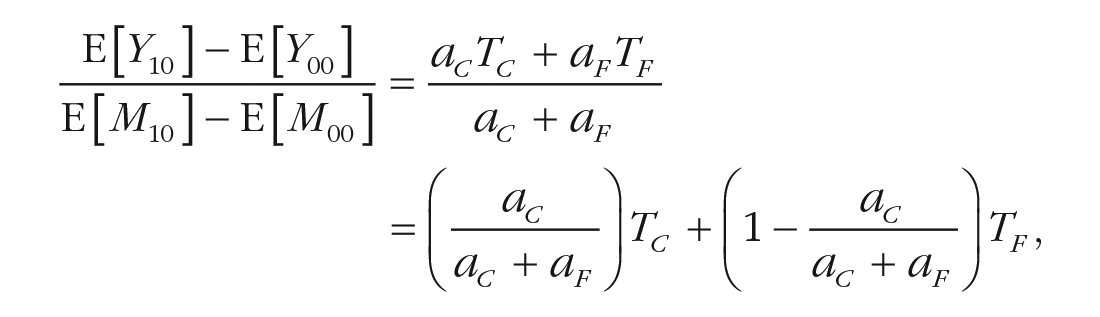
\begin{array}{l} \frac{E [Y_{10}] - E [Y_{00}]}{E [M_{10}] - E [M_{00}]} = \frac{a_{C} T_{C} + a_{F} T_{F}}{a_{C} + a_{F}} \\ = (\frac{a_{C}}{a_{C} + a_{F}}) T_{C} + (1 - \frac{a_{C}}{a_{C} + a_{F}}) T_{F}, \end{array}

and the corresponding result for the second encouragement is

\begin{array}{l} \frac{E [Y_{01}] - E [Y_{00}]}{E [M_{01}] - E [M_{00}]} = \frac{a_{C} T_{C} + a_{S} T_{S}}{a_{C} + a_{S}} \\ = (\frac{a_{C}}{a_{C} + a_{S}}) T_{C} + (1 - \frac{a_{C}}{a_{C} + a_{S}}) T_{S} . \end{array}

This formalization shows the conditions under which one will be able to detect heterogeneous effects of the mediator. For example, if a_F = 0, the shares of each group are identified, as are the effects of M on Y for full compliers (T_C) and second-instrument compliers (T_S). An analogous result holds if one instead stipulates a_S = 0, in which case, T_C and T_F can be identified.

What does this result imply for experimental design? Researchers seeking to estimate the effects of M on Y for different groups of compliers may wish to devise encouragements of varying intensity. A weak encouragement (X₁ = 1) may induce a psychological state M = 1 among subjects who are highly attentive and pliable (i.e., always-takers and full compliers); a stronger encouragement (X₂ = 1) may induce this psychological state as well among the less attentive and pliable, such that M = 1 among always-takers, full compliers, and second-instrument compliers. This design enables a researcher to estimate both T_C and T_S, which allows a direct assessment of effect heterogeneity among different groups of compliers. The precision with which these parameters are estimated will depend on the group sizes, a_C and a_S. Ideally, half the subject pool would be full compliers and half second-instrument compliers. In practice, a series of experiments may be necessary to develop encouragements that induce the mediating state among ever larger shares of subjects.

What if mounting experimental evidence suggests that treatment effect heterogeneity is limited? Two-stage least squares regression takes advantage of both instruments to produce an efficient estimate of M’s effect on Y (Angrist & Pischke, 2009, pp. 173–175). The 2SLS estimator renders a weighted average of the effects of M among different complier subgroups. The fact that two instruments are used to reveal a single causal effect means that there is excess information that can be used to test the statistical adequacy of the assumption of homogeneous effects (Angrist et al., 2000; Wooldridge, 2010, pp. 134–137).

To summarize, designs that employ multiple encouragements can be valuable for two reasons. First, they allow a researcher to examine indirect effects that are transmitted via multiple mediators (up to a limit of one mediator per encouragement). Second, they facilitate the investigation of treatment effect heterogeneity across different sets of compliers. A comprehensive research program would endeavor to do both, investigating each pathway using multiple encouragements.

Example: using multiple encouragements to estimate the effects of multiple mediators

To illustrate the scaling phase of implicit mediation when multiple instruments are used to investigate multiple mediators, we turn again to Gaesser et al. (2020). Recall that all subjects in their experiments are presented with a short passage of text that describes a stranger in need. In the control group, subjects are asked to critique the style of the passage; in the baseline treatment condition, they are instead asked to imagine helping the person, “creating a vivid and elaborate event where you strongly see the scenario in your mind’s eye” (Gaesser et al., 2020 online materials). The baseline treatment increases subjects’ actual willingness to help, and the authors posited that its effect is mediated by three factors: perspective-taking, helping-scene vividness, and person vividness (the self-reported vividness of the person whom one imagines). In Experiment 3 (p. 693), the authors introduced two new treatments to probe these possibilities. In the “imagine contact” treatment, subjects were asked to “imagine yourself meeting this stranger for the first time in a scenario before the one described below,” i.e., before the stranger is in need. And in the “person only” treatment, they are asked to “imagine the person in the scenario as if they were looking at them in a photo with a blank background.” In neither of these alternative conditions are subjects instructed to imagine helping the person or to visualize the scene. We thus have three potential mediators and three IVs.¹⁷

The exploratory phase of implicit mediation can teach us something about the extent to which each potential mediator is likely to be an actual mediator. Using OLS to regress each potential mediator on the three treatments will indicate the effects of the treatments on the mediators. And we can again use OLS to regress the outcome of interest, willingness to help, on the three treatments. The combination of results that we obtain from these two sets of regressions will be informative. (See Table 1.) To evaluate the extent to which these mediators affect Y, we turn to the scaling phase.

Table 1.

Possible Implicit-Mediation Findings

Result	Inference	Rationale
X affects M and Y	M may be a mediator.	X appears to influence M, and this effect seems to coincide with a change in Y, as would be expected if M were a mediator.
X affects M but not Y	M appears not to be a mediator.	Although X affects M, this effect seems not to have any consequences for Y.
X affects Y but not M	Some variable other than M may be a mediator.	X appears to have no effect on M, which means that X’s apparent effect on Y is not due to changes in M.
X affects neither M nor Y	There seem to be no indirect pathways from X to Y through M or other mediators.	X seems not to set in motion any causal effects.

Note: In all cases, X is manipulated by adding features that trigger or block mediation pathways. M is the proposed mediator, and Y is the outcome of interest. When we say that one variable does not affect another (e.g., “X affects M but not Y”), we are speaking of average effects. It remains possible that the first variable affects the second in different ways for different people and that these effects cancel out—hence the importance of confirming the apparent lack of effect by examining treatment-effect heterogeneity of X on M and X on Y.

Assume that in the exploratory phase, we find that each of the treatments affects Y and some combination of the mediators. We then begin the scaling phase by considering whether these treatments satisfy the exclusion restriction. Perhaps we are unwilling to assume that they do: Perhaps we believe that they affect Y partly through some fourth, unmeasured mediator. In this case, the implicit-mediation analysis halts until we obtain a measure of this fugitive mediator and craft a fourth encouragement. But suppose instead that we are willing to make the exclusion restriction in each case: We assume that these treatments affect willingness to help exclusively through some combination of the three mediators. In this case, we can proceed. Because the treatments are randomized, the independence assumption is satisfied by design. In the exploratory phase, our regression of M on the treatments showed that each treatment affected M; in other words, the first-stage condition is also satisfied. And if we grant that each of the treatments moves the mediators in only one direction (relative to a control condition), the monotonicity assumption is satisfied as well. The three treatments are thus assumed to be IVs, and we can estimate the effects of the three mediators among compliers.¹⁸

Table 2 depicts the results of this implicit-mediation analysis. The first three columns are part of the exploratory phase: They are first-stage regressions, indicating the effects of the three treatments on the potential mediators. We see from these regressions that the treatments affect each potential mediator, which bolsters the case that the treatments’ effects are transmitted through these variables. In addition, the results make theoretical sense. The baseline treatment, in which subjects are instructed to imagine helping the stranger in as much detail as possible, leads to much more helping-scene vividness than the other treatments. By contrast, telling subjects to focus on only a person, rather than on the totality of the narrative description (as in the control condition), decreases helping-scene vividness.¹⁹

Table 2.

Implicit Mediation Analysis in Gaesser et al. (2020), Experiment 3

	First-stage regressions						Reduced-form regression		Instrumental variables regression
	Helping-scene vividness		Person vividness		Perspective-taking		Willingness to help		Willingness to help
Intercept	−0.39	0.09	−0.93	0.09	−0.84	0.09	−0.32	0.07	0.00	0.03
Baseline treatment	1.63	0.10	1.21	0.11	1.45	0.10	0.98	0.09
Imagine-prior-contact treatment	0.40	0.13	1.23	0.11	0.93	0.12	0.41	0.10
Person-only treatment	−0.44	0.13	1.43	0.10	1.09	0.11	−0.09	0.10
Helping-scene vividness									0.63	0.12
Person vividness									0.41	0.31
Perspective-taking									−0.37	0.39
R²	.16		.15		.12		.06
F	182.17		69.72		68.33		68.34
Standard error of regression	3.27		1.94		2.39		3.00
N subjects	1,115		1,115		1,115		1,115		1,115
N observations	11,150		11,150		11,150		11,150		11,150

Note. Entries in the first four columns are OLS estimates and standard errors. Entries in the last column are IV estimates and standard errors. Each subject was assigned to a control condition or to one of the three treatments listed here. Helping-scene vividness, person vividness, and perspective-taking are the three potential mediators; see page 12 of this article. Each subject responded to 10 scenarios, and standard errors are clustered at the level of the subject.

The fourth column of Table 2 is also part of the exploratory phase. It is the regression of the outcome of interest, willingness to help, on the treatments. This regression yields estimates of the total effect of each treatment on the outcome (in IV parlance, these are “reduced-form” effects). The estimates indicate that the baseline treatment and the “imagine positive contact” treatment both increased willingness to help, while the person-only treatment did not. Furthermore, the baseline treatment, which has by far the strongest effect on helping-scene vividness, also has by far the strongest effect on willingness to help. Taken together, these exploratory phase results suggest that helping-scene vividness and perspective-taking may both be mediators and that helping-scene vividness may be especially important. The results are less consistent with person vividness being a mediator because the person-only treatment, which strongly predicts person vividness, has a weak total effect on the outcome, willingness to help. To sort out the multivariate relationships between the mediators and the outcome, we turn to the scaling phase.

The final column of Table 2 depicts the results of the scaling phase. Assuming that the treatments affect willingness to help exclusively through the three posited mediators, we find that helping-scene vividness has a powerful effect on willingness to help, at least among participants whose thinking about the scene can be made more vivid by the treatments. The role of person vividness is ambiguous given the standard errors. Perspective-taking seems not to increase willingness to help.

Implicit mediation is, in sum, an approach to the study of mediation that is feasible in a wide array of psychological studies. But, of course, it is not the only experimental approach to mediation analysis. (See Glynn, 2021, for a survey of recent advances in this area.) We turn now to distinguishing it from other experimental approaches, beginning with one that has attracted recent attention from statisticians: (e.g., Imai et al., 2013) the parallel-design approach.

Other Experimental Approaches

Parallel-design experiments (e.g., Imai et al., 2013) begin with the random assignment of subjects to Study A or Study B. In Study A, only X is randomly assigned (e.g., have some people write about the scene imagery while others complete a placebo task). In Study B, both X and M are randomly assigned. Study A thus furnishes an estimate of the total effect of X on Y, and Study B thus furnishes an estimate of the direct effect of X on Y: the effect of X on Y that is not transmitted through M. The difference between these two estimates can itself be taken as an estimate of the indirect effect.

In principle, parallel designs are simple. But in practice, they are much more difficult to implement than implicit-mediation approaches. To begin, Studies A and B must be conducted with the same sample at approximately the same time (i.e., “in parallel”). Second, one must also invoke the no-interaction assumption: The direct effect of X on Y for any subject cannot depend on the value of M (Imai et al., 2013, p. 13).²⁰

Third, and most forbidding, one must directly manipulate the mediator. And not any manipulation will suffice. Instead, one must devise a manipulation that sets each value of the mediator to a specific value such that every subject in the experiment is a complier. And as with encouragement designs, this manipulation must affect the mediator of interest without affecting any other possible mediators. Because most psychological mediators are intangible, they are hard to manipulate with precision, and the requirement thus seems a very tall order. The formidable demands of this approach may account for the paucity of direct manipulations of mediators in psychology experiments.²¹

Several other experimental designs have been suggested for the study of mediation, and it is useful to recognize how they, too, overlap with and depart from implicit-mediation analysis. Moderation-of-process designs (Spencer et al., 2005), also called experimental blockage or enhancement designs (Pirlott & MacKinnon, 2016, pp. 31–32) or testing-a-process-by-an-interaction designs (Jacoby & Sassenberg, 2011), are unlike implicit-mediation analysis in a fundamental way: They involve a manipulation of the mediator that is distinct from the manipulation of the treatment. In that sense, these designs are more akin to parallel designs.²²

The two-phase nature of implicit-mediation analysis makes it an experimental-causal-chain design (e.g., Spencer et al., 2005; Stone-Romero & Rosopa, 2008). But to our knowledge, it is distinct from other designs of this type that have been proposed. For example, other designs of this sort require that one “manipulate both the proposed independent variable and the proposed psychological process,” i.e., the potential mediator (Spencer et al., 2005, p. 846); the emphasis on direct manipulation of the mediator in most of these designs sets them apart from implicit-mediation analysis, which instead relies on encouragements. Implicit-mediation analysis also differs from other causal-chain designs in its use of IV estimation, and it therefore requires that there be no direct path between the encouragement and the outcome. By contrast, causal-chain designs rely on regression of Y on M to find the effect of M.²³

The designs most similar to the exploratory phase of implicit-mediation analysis are the dismantling and build-up (or constructive) designs advanced by West and Aiken (1997; see also West et al., 1993). They seem to be seldom used; for example, our content analysis indicates that no examples of these designs were published in JPSP in 2019. Like implicit-mediation analysis, these designs call for the creation of a set of treatments: a baseline treatment and alternative treatments from which components are added or removed. But unlike implicit-mediation designs, dismantling and build-up designs are analyzed via standard measurement-of-mediation statistical methods (e.g., West et al., 1993, pp. 591–597) to apportion the total effect of X on Y to direct and indirect effects. As we have argued, this framework is prone to bias. The exploratory phase of implicit-mediation analysis differs in that it advises scholars to refrain from regressing outcomes on confounded mediators. It calls on them to instead make inferences about mediation on the basis of the pattern of effects observed when X is manipulated in different ways. (See Table 1.) Scholars may then proceed to the scaling phase, in which they estimate the effects on Y of X-induced changes in M. If the exclusion restriction holds, these estimates will be estimates of the indirect effect of X on Y. There is no analog in dismantling and build-up designs to this second phase of implicit-mediation analysis.

To facilitate a head-to-head comparison of the experimental approaches discussed in this section, Table 3 summarizes the leading designs on three dimensions: whether they require manipulation of the mediator, whether the treatment and mediator are manipulated simultaneously (if the mediator is manipulated at all), and the statistical method that is to be used to analyze the experimental results. The upshot of Table 3 is that implicit mediation shares some features with other experimental approaches but is distinctive when the three criteria are considered jointly.

Table 3.

Experimental Designs for Mediation Analysis

Names	Manipulation of mediator (distinct from manipulation of treatment)?	Treatment and mediator manipulated simultaneously?	Method of inference about indirect effects
Blockage and enhancement; moderation of process; testing a process by an interaction	Yes	Yes	Examine the effect of the interaction of X and M on Y.
Parallel designs; double randomization	Yes	Yes, but only in one arm of these two-arm (hence “parallel”) designs	Difference of means; see Imai et al. (2013) for details.
Experimental causal chain	Yes	No	No direct statistical inference about indirect effects; instead, draw inferences from each manipulation of the treatment using ordinary least squares (in the exploratory phase) or instrumental variables regression (in the scaling phase).
Dismantling and build‑up; constructive designs	No	No	Measurement-of-mediation methods (e.g., Baron & Kenny, 1986).
Implicit mediation	No	No	No direct statistical inference about indirect effects; instead, draw inferences from each manipulation of the treatment using ordinary least squares or instrumental variables regression.

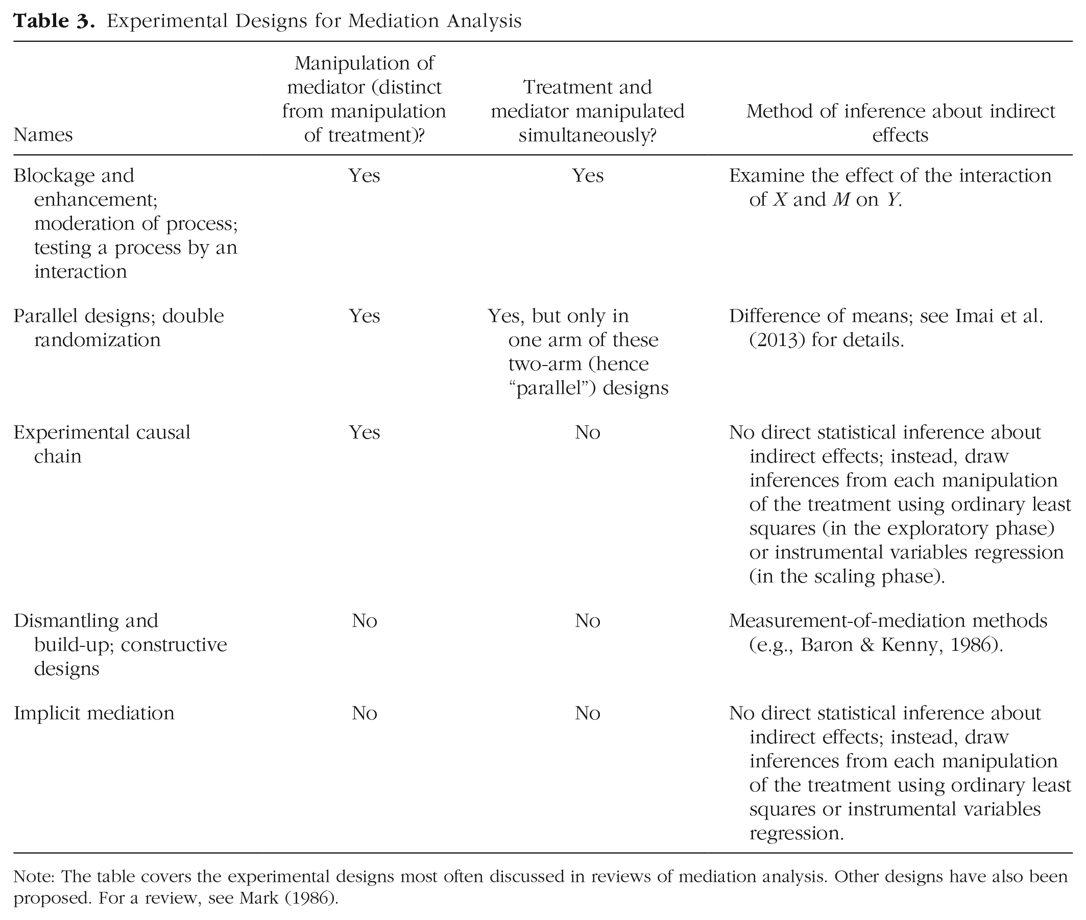
Note: The table covers the experimental designs most often discussed in reviews of mediation analysis. Other designs have also been proposed. For a review, see Mark (1986).

Conclusion

The challenge of conducting a convincing demonstration that M mediates the effect of X on Y is much more difficult than many scholars realize. Measurement-of-mediation analysis is ubiquitous, but as our content analysis has shown, authors only rarely discuss or defend the assumptions underlying this type of analysis. And ironically, when scholars do address mediation-focused methodological issues, the statistical methods they employ address only second-order concerns, such as obtaining more accurate standard errors through bootstrapping or hierarchical modeling. This is a bit like rearranging the deck chairs on the Titanic. If the estimates are systematically prone to bias, even the most sophisticated standard errors may badly understate the average estimation error.

Scholars seem to have lost sight of the fact that measurement-of-mediation analysis relies on dubious assumptions. Because M is not randomly assigned, the relationship between M and Y is not a reliable guide to M’s effect on Y. Measurement-of-mediation analysis exaggerates the effect of M on Y (and understates the direct effect of X on Y) when unobserved factors that affect the mediator are positively correlated with unobserved causes of the outcome. We are unaware of published articles in psychology in which authors argued persuasively that cov(e₁,e₃) is zero for their application.

To make matters worse, between-subjects variation in the effects of X on M and of M on Y upends the usual algebra by which total effects are partitioned into direct and indirect effects. It is easy to formulate scenarios by which measurement-of-mediation “demonstrates” that M mediates the effect of X on Y even though the data were generated in such a way that M plays no mediating role whatsoever for any subject.

We recommend a return to basics: experimental design. At the same time, we are quick to acknowledge the practical constraints under which experimental psychologists operate. Direct experimental manipulation of a given mediator is rarely a viable option. And the challenge of setting M to specific values is even more formidable when researchers must do so without inadvertently influencing other mediators.

A more cautious approach is implicit mediation. In a nutshell, implicit-mediation designs add or subtract ingredients from X in ways that illuminate the causal pathways that link X to Y. The most attractive feature of these designs is that they stay within the constraints of conventional experimental inference: Variants of X are randomly assigned, and their effects on possible mediators and outcomes are assessed. The exploratory phase of implicit mediation can help to rule out possible mediators by showing the lack of apparent effect of X on a specific M both on average and for particular subgroups. The scaling phase makes explicit the assumptions that allow a researcher to make causal claims about M’s effect on Y, at least for certain subgroups. Although these are strong assumptions, implicit mediation facilitates a cumulative and comparatively agnostic research program in which researchers propose and test variants of X that switch on or off mediating pathways in an effort to discern which pathways, when activated, reliably change Y. Given the shortcomings of measurement-of-mediation approaches and the practical difficulties of directly manipulating mediators, implicit-mediation designs merit more attention than they have received.

Supplemental Material

sj-pdf-1-amp-10.1177_25152459211047227 – Supplemental material for The Failings of Conventional Mediation Analysis and a Design-Based Alternative

Supplemental material, sj-pdf-1-amp-10.1177_25152459211047227 for The Failings of Conventional Mediation Analysis and a Design-Based Alternative by John G. Bullock and Donald P. Green in Advances in Methods and Practices in Psychological Science

Footnotes

Acknowledgements

We thank Jennifer Lin for research assistance and Mina Cikara, Brendan Gaesser, Robin Gomila, Macartan Humphreys, Roni Porat, and Teppei Yamamoto for helpful comments and discussions.

Transparency

Action Editor: Mijke Rhemtulla

Editor: Daniel J. Simons

Author Contributions

J.G. Bullock and D.P. Green jointly generated the idea for this article, wrote the code for the simulations, analyzed the data, and verified the accuracy of the analyses. They jointly wrote the first draft of the manuscript and edited it. Both authors approved the final submitted version of the manuscript.

ORCID iD

John G. Bullock

Supplemental Material

Additional supporting information can be found at

Notes

References

Angrist

J. D.

Graddy

Imbens

G. W.

(2000). The interpretation of instrumental variables estimators in simultaneous equations models with an application to the demand for fish. The Review of Economic Studies, 67(3), 499–527.

Angrist

J. D.

Imbens

G. W.

(1995). Two-stage least squares estimation of average causal effects. Journal of the American Statistical Association, 90(430), 431–442.

Angrist

J. D.

Imbens

G. W.

Rubin

D. B.

(1996). Identification of causal effects using instrumental variables. Journal of the American Statistical Association, 91(434), 444–455.

Angrist

J. D.

Pischke

J.-S.

(2009). Mostly harmless econometrics. Princeton University Press.

Baron

R. M.

Kenny

D. A.

(1986). The moderator-mediator variable distinction in social psychological research: Conceptual, strategic, and statistical considerations. Journal of Personality and Social Psychology, 51(6), 1173–1182.

Bitterly

T. B.

Schweitzer

M. E.

(2020). The economic and interpersonal consequences of deflecting direct questions. Journal of Personality and Social Psychology, 118(5), 945–990.

Brainerd

Chang

Bialer

(2020). From association to gist. Journal of Experimental Psychology: Learning, Memory, and Cognition, 46(11), 2106–2127. https://doi.org/10.1037/xlm0000938

Bullock

J. G.

Green

D. P.

S. E.

(2010). Yes, but what’s the mechanism? (Don’t expect an easy answer). Journal of Personality and Social Psychology, 98(4), 550–558.

Cikara

Bruneau

E. G.

Saxe

R. R.

(2011). Us and them: Intergroup failures of empathy. Current Directions in Psychological Science, 20(3), 149–153.

10.

Gaesser

Dodds

Schacter

D. L.

(2017). Effects of aging on the relation between episodic simulation and prosocial intentions. Memory, 25(9), 1272–1278.

11.

Gaesser

Shimura

Cikara

(2020). Episodic simulation reduces intergroup bias in prosocial intentions and behavior. Journal of Personality and Social Psychology, 118(4), 683–705.

12.

Gerber

A. S.

Green

D. P.

(2012). Field experiments: Design, analysis, and interpretation. W.W. Norton.

13.

Glynn

A. N.

(2012). The product and difference fallacies for indirect effects. American Journal of Political Science, 56(1), 257–269.

14.

Glynn

A. N.

(2021). Advances in experimental mediation analysis. In Druckman

Green

(Eds.), Advances in experimental political science (pp. 257–270). Cambridge University Press. https://doi.org/10.1017/9781108777919.019

15.

Guo

Sun

Cai

Zhang

Song

(2019). Why are smarter individuals more prosocial? A study on the mediating roles of empathy and moral identity. Intelligence, 75, 1–8.

16.

Harmon-Jones

Hinton

Tien

Summerell

Bastian

(2019). Pain offset reduces rumination in response to evoked anger and sadness. Journal of Personality and Social Psychology, 117(6), 1189–1202.

17.

Herlitz

Yonker

J. E.

(2002). Sex differences in episodic memory: The influence of intelligence. Journal of Clinical and Experimental Neuropsychology, 24(1), 107–114.

18.

Imai

Tingley

Yamamoto

(2013). Experimental designs for identifying causal mechanisms. Journal of the Royal Statistical Society: Series A (Statistics in Society), 176(1), 5–51.

19.

Jacoby

Sassenberg

(2011). Interactions do not only tell us when, but can also tell us how: Testing process hypotheses by interaction. European Journal of Social Psychology, 41(2), 180–190.

20.

Judd

C. M.

Kenny

D. A.

(1981). Process analysis: Estimating mediation in treatment evaluations. Evaluation Review, 5(5), 602–619.

21.

MacKinnon

D. P.

(2008). Introduction to statistical mediation analysis. Erlbaum.

22.

MacKinnon

D. P.

Lockwood

C. M.

Hoffman

J. M.

West

S. G.

Sheets

(2002). A comparison of methods to test mediation and other intervening variable effects. Psychological Methods, 7(1), 83–104.

23.

Mark

M. M.

(1986). Validity typologies and the logic and practice of quasi-experimentation. New Directions for Program Evaluation, 1986(31), 47–66.

24.

Pirlott

A. G.

MacKinnon

D. P.

(2016). Design approaches to mediation analysis. Journal of Experimental Social Psychology, 66, 29–38.

25.

Robins

J. M.

Greenland

(1992). Identifiability and exchangeability for direct and indirect effects. Epidemiology, 143–155.

26.

Rosenbaum

P. R.

(1984). The consequences of adjustment for a concomitant variable that has been affected by the treatment. Journal of the Royal Statistical Society A, 147(5), 656–666. https://doi.org/10.2307/2981697

27.

Rubin

D. C.

Umanath

(2015). Event memory: A theory of memory for laboratory, autobiographical, and fictional events. Psychological Review, 122(1), 1–23. https://doi.org/10.1037/a0037907

28.

Schochet

P. Z.

(2020). The complier average causal effect parameter for multiarmed RCTs. Evaluation Review, 44(5–6), 410–436.

29.

Sobel

M. E.

(2008). Identification of causal parameters in randomized studies with mediating variables. Journal of Educational and Behavioral Statistics, 33(2), 230–251.

30.

Spencer

S. J.

Zanna

M. P.

Fong

G. T.

(2005). Establishing a causal chain: Why experiments are often more effective than mediational analyses in examining psychological processes. Journal of Personality and Social Psychology, 89(6), 845–851.

31.

Stone-Romero

E. F.

Rosopa

P. J.

(2008). The relative validity of inferences about mediation as a function of research design characteristics. Organizational Research Methods, 11(2), 326–352.

32.

T.-T.

Superchi

Boutron

Vansteelandt

(2020). The conduct and reporting of mediation analysis in recently published randomized controlled trials: Results from a methodological systematic review. Journal of Clinical Epidemiology, 117, 78–88.

33.

West

S. G.

Aiken

L. S.

(1997). Toward understanding individual effects in multicomponent prevention programs: Design and analysis strategies. In Bryant

K. J.

Windle

West

S. G.

(Eds.), The science of prevention: Methodological advances from alcohol and substance abuse research (pp. 167–209). American Psychological Association. https://doi.org/10.1037/10222-006

34.

West

S. G.

Aiken

L. S.

Todd

(1993). Probing the effects of individual components in multiple component prevention programs. American Journal of Community Psychology, 21(5), 571–605.

35.

Wooldridge

J. M.

(2010). Econometric analysis of cross section and panel data (2nd ed.). MIT Press.

36.

Zanna

M. P.

Cooper

(1974). Dissonance and the pill: An attribution approach to studying the arousal properties of dissonance. Journal of Personality and Social Psychology, 29(5), 703–709.

Supplementary Material

Please find the following supplemental material available below.

For Open Access articles published under a Creative Commons License, all supplemental material carries the same license as the article it is associated with.

For non-Open Access articles published, all supplemental material carries a non-exclusive license, and permission requests for re-use of supplemental material or any part of supplemental material shall be sent directly to the copyright owner as specified in the copyright notice associated with the article.

0.00 MB

0.42 MB