
Abstract
Methodological innovations have allowed researchers to consider increasingly sophisticated statistical models that are better in line with the complexities of real-world behavioral data. However, despite these powerful new analytic approaches, sample sizes may not always be sufficiently large to deal with the increase in model complexity. This difficult modeling scenario entails large models with a limited number of observations given the number of parameters. Here, we describe a particular strategy to overcome this challenge: regularization, a method of penalizing model complexity during estimation. Regularization has proven to be a viable option for estimating parameters in this small-sample, many-predictors setting, but so far it has been used mostly in linear regression models. We show how to integrate regularization within structural equation models, a popular analytic approach in psychology. We first describe the rationale behind regularization in regression contexts and how it can be extended to regularized structural equation modeling. We then evaluate our approach using a simulation study, showing that regularized structural equation modeling outperforms traditional structural equation modeling in situations with a large number of predictors and a small sample size. Next, we illustrate the power of this approach in two empirical examples: modeling the neural determinants of visual short-term memory and identifying demographic correlates of stress, anxiety, and depression.
The empirical sciences have seen a rapid increase in data collection, both in the number of studies conducted and in the richness of data within each study. With large numbers of variables available, researchers often want to go beyond what their hypothesis-driven models tested and explore which variables are most informative in explaining observed variability in the outcome of interest. Typical questions asked are “What is the importance of my variables for predicting the outcome of interest?” and, ultimately, “What subset of variables is most predictive of (or most relevant for) that outcome?”
How to select a subset of variables for modeling purposes (variable selection) is a pervasive challenge in applied statistics. In the field of statistical learning (also known as machine learning or data mining), a large amount of attention has been dedicated to the topic of how predictors can be optimally selected when there is little or no prior knowledge. Statistical approaches to variable selection range from the notorious stepwise variable-selection procedures (cf. Thompson, 1995) to more complex and comprehensive approaches, such as support vector machines and random forests. One particularly fruitful approach is regularized regression, a method that solves the variable-selection problem by adding a penalty term that penalizes solutions, effectively producing sparse solutions in which only few predictors are allowed to be “active.” Regularization approaches vary in their precise specifications and include methods such as ridge (Hoerl & Kennard, 1970), lasso (least-absolute-shrinkage-and-selection operator; Tibshirani, 1996), and elastic-net (Zou & Hastie, 2005) regression.
Despite their strengths, these regularization approaches are generally developed in a context of models that include only observed indicators and consequently do not allow for modeling measurement error. However, incorporation of measurement error is central to many approaches in psychology. The most dominant approach to incorporating measurement error in psychology and related fields is the use of structural equation modeling (SEM). SEM offers a general framework in which hypotheses can be formulated at the construct (latent) level and explicit measurement models link the observed variables to the latent constructs. Latent-variable models account for measurement error, assess reliability and validity, and often have greater generalizability and statistical power than methods based on observed variables (e.g., Brandmaier, Wenger, Raz, & Lindenberger, 2018; Little, Lindenberger, & Nesselroade, 1999). Here we describe a novel approach called regularized SEM, which incorporates the strengths of regularization into the SEM framework, allowing researchers to estimate sparse model solutions and implicitly solve large-scale variable selection in SEM by introducing a penalized likelihood function. We use simulations and two empirical data sets to illustrate the performance of regularized SEM and discuss practical aspects of using the method for modeling empirical data. First, though, we outline the general principles of regularization and discuss how to extend these principles to SEM.
Regularization Overview
Regularization in the context of regression
To set the stage for discussing the use of regularization (e.g., shrinkage or penalized estimation) in structural equation models, we give a brief overview in the context of regression. (For more detail, interested readers may consult McNeish, 2015, or Helwig, 2017.) We use ordinary least squares (OLS) estimation as a basis for our discussion. Given N continuous observations of P predictors in matrix X and associated continuous outcome Y, one can estimate the regression coefficients by minimizing the residual sum of squares (RSS) as follows:

For coefficients, one estimates an intercept β0 along with β j coefficients (one for each of the P predictors). However, there may be instances when a simpler model—that is, one that includes fewer predictors—is preferred. To select the variables for this simpler model, one can use the lasso (Tibshirani, 1996). Lasso regularization builds upon Equation 1, incorporating a penalty for each parameter (larger parameter values incur a larger penalty):

The lasso penalty includes the traditional RSS as in Equation 1, but introduces two new components. First and foremost, it introduces a new penalty term that reflects the sum of all beta coefficients (the right-hand term in Equation 2). In this manner, much as how a traditional regression attempts to minimize the squared residuals, the lasso penalty tries to drive parameters to zero, thus implicitly performing variable selection. Second, as can be seen in Equation 2, the sum of the absolute values of the β j coefficients is multiplied by a hyperparameter, λ. This term quantifies the influence of the lasso penalty on the overall model fit and thus weights the importance of the least squares fit versus the importance of the lasso penalty: As λ increases, a stronger penalty is incurred for each parameter, which results in greater shrinkage of the coefficient sizes. The λ term is called a hyperparameter because it cannot be estimated jointly with the β j coefficients (this is not the case in Bayesian regularization, which we return to shortly). As there is no generally optimal value for λ, it is common to test a range of λ values, combined with cross-validation, to examine what the most appropriate degree of regularization is for a given data set.
Another type of regularization is ridge regularization (Hoerl & Kennard, 1970). In contrast to the lasso, the ridge sums the squared coefficients. Whereas the lasso penalty will push the betas all the way to zero (as any nonzero beta will contribute to the penalty term), the ridge penalty will instead shrink the betas, but not necessarily all the way to 0 (as the squaring operation means that small betas incur negligible penalties). One benefit of ridge regularization is that it better handles multicollinearity among predictors.
In an effort to combine the variable-selection aspects of the lasso with the ridge regularization’s ability to handle collinearity, Zou and Hastie (2005) proposed the elastic net. Through the use of a mixing parameter, α, the elastic net combines ridge and lasso regularization:

Much as different values of λ, combined with cross-validation, can be tested to choose a final model, different values of α can be tested. Generally, the values tested range from zero (equivalent to the ridge penalty) to 1 (equivalent to the lasso penalty).
Extensions
Originating from the application of ridge regression as a way to improve the results of OLS when predictors are correlated (Hoerl & Kennard, 1970), a large number of alternative forms of regularization have been proposed. In the case of high-dimensional research scenarios, sparser versions of the lasso have been proposed. These include the adaptive lasso (Zou, 2006), the smoothly clipped absolute deviation penalty (Fan & Li, 2001), and the minimax concave penalty (Zhang, 2010), to name a few. Methods such as these have been shown to produce more optimal results than the lasso when only a small number of predictors among thousands of candidates or more are desired to have nonzero coefficients. In general, there is no optimal type of regularization, as each type is optimal under different assumptions.
An additional way that regularization methods have been extended is with Bayesian estimation. In Bayesian regression, prior distributions are placed on all the coefficients in the model. When these priors are diffuse (large variances), the observed data have a large influence on the posterior distribution of each parameter. Regularization as applied to Bayesian estimation entails placing different types of prior distributions on those parameters of interest and constraining the width of these priors to shrink the coefficients toward zero. Thus, prior knowledge, as applied through strong priors, carries greater weight in determining the posterior distribution for each parameter when regularization is applied. Placing normal-distribution priors has been shown to be equivalent to ridge regression (Kyung, Gill, Ghosh, & Casella, 2010; T. Park & Casella, 2008; Tibshirani, 1996), whereas the lasso corresponds to Laplace distribution priors (T. Park & Casella, 2008; Tibshirani, 1996). Particularly when variable selection is desired, a number of more advanced forms of Bayesian regularization have been found to perform better than the Bayesian version of the lasso (see van Erp, Oberski, & Mulder, 2018, for an overview).
The Rationale for Regularization
Traditionally, a test statistic (and associated p value) is used to determine the significance of a parameter. In regression with regularization, one instead tests a sequence of penalties, compares models to choose a best-fitting model, and examines whether the parameter estimates in this best model are nonzero. Nonzero coefficients can be thought of as important (e.g., see Laurin, Boomsma, & Lubke, 2016). This approach stands in stark contrast to the use of p values, as using regularization to label parameters as important does not rely on any asymptotic foundations (there are no statements with regard to a population). In particular, because the regularized estimates move away from the point of maximum likelihood, asymptotic distributions of parameter estimates do not hold any more. Commonly paired with cross-validation, regularization attempts to identify which parameters are likely to be nonzero not only in the current sample, but also in a hold-out sample.
Sparsity is an implicit conceptual assumption of regularization methods, such as the lasso, that set parameters to zero (e.g., Hastie, Tibshirani, & Wainwright, 2015). In other words, this approach reflects the hypothesis that the true underlying model has few nonzero parameters. However, in psychological research, this is unlikely to be true. Instead, most variables in a data set likely have small correlations among themselves (e.g., the “crud” factor—Meehl, 1990). As a result, the use of regularization in psychological research will impart some degree of bias into the results; as with all procedures, there is no such thing as a “free lunch” (Wolpert & Macready, 1997). Although this may at first seem to be an undesirable side effect, we argue that there are common situations in which the benefits of reduced variance outweigh the drawbacks of nonzero degrees of bias. First, we provide a brief overview of the bias-variance trade-off.
Bias-variance trade-off
Although regularization is often used when variable selection is desired to achieve a parsimonious level of description, or when the number of predictors is larger than the sample size, one of the fundamental motivations behind regularization concerns the bias-variance trade-off. Bias refers to whether estimates or predictions are, on average (across many random draws from the population), equal to the true values in the population. Variance, on the other hand, refers to the variability, or precision, of these estimates (see Yarkoni & Westfall, 2017, for further discussion). Practically speaking, researchers want bias to be absent and variance to be low (e.g., the Gauss-Markov theorem guarantees that least squares estimation yields unbiased estimates with the lowest variance among all unbiased linear estimators); however, it can be difficult to achieve both goals in practice. Regularization plays a role when one wishes to allow for some bias in order to achieve a larger decrease in variance. When the sample size may be insufficient to adequately test the number of predictors the researcher desires to include in the model, regularization will systematically bias the regression coefficients toward zero, as the variance of the estimator will be high because of the low sample size. Such an approach will prove particularly beneficial when the true model is sparse (i.e., only few predictors are important).
To provide a simple example, we simulated 30 observations with 10 predictors of a normally distributed outcome variable. This 3-to-1 (30-to-10) ratio is far below recommended guidelines for regression models. Across 1,000 repetitions, the first predictor was simulated to have the strongest regression coefficient (.5), the second predictor was simulated to be half as strong (.25), and the third predictor was simulated to be half as strong as the second (.125). The other 7 predictors had simulated coefficients of zero. The resultant coefficients from both OLS and ridge regression models are displayed in Figure 1.
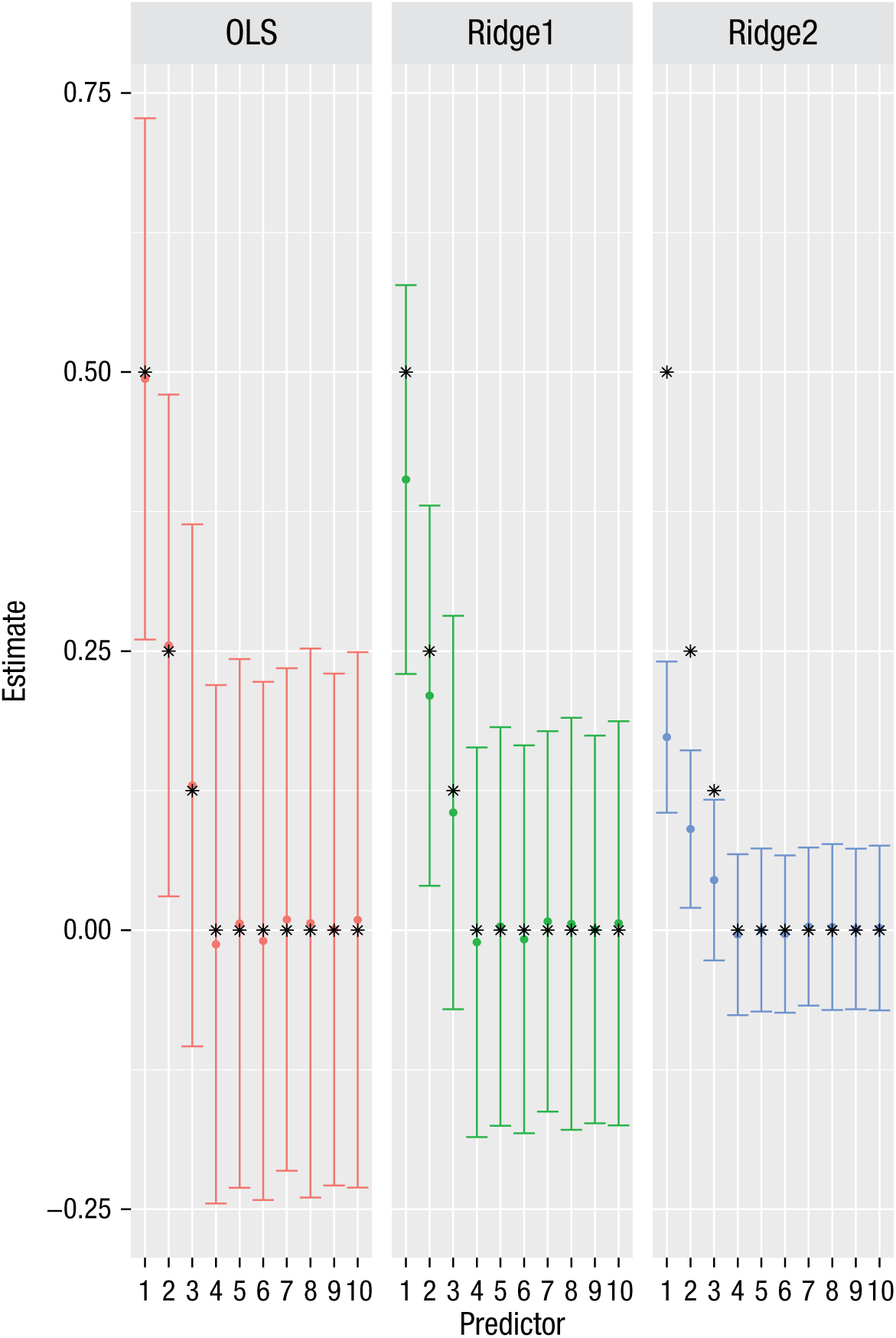
Illustration of the bias-variance trade-off: parameter estimates from models fit to simulated data. The simulation involved 1,000 repetitions of 30 observations with 10 predictors of a normally distributed outcome variable. Results from an ordinary least squares (OLS) model and two ridge regressions (a weaker penalty of 5 for Ridge1 and a stronger penalty of 50 for Ridge2) are shown. The error bars show ±1 SD of the estimate for each parameter. Asterisks denote the simulated parameter estimates.
The figure shows that the estimates from the OLS model are unbiased (i.e., the mean parameter estimates correspond with the simulated parameter estimates). However, the absence of bias comes at the expense of variance, as the OLS coefficients have a large degree of variability. This is to be expected given the results of methodological work on sample sizes in linear regression (Green, 1991). However, instead of restricting the number of predictors entered into the model in order to address a small fixed sample size (e.g., testing only 2 predictors when testing all 10 is desired), researchers can use regularization to impart bias as a mechanism to decrease the variance of the estimates. In contrast to the OLS results, the ridge parameter estimates are biased toward zero (i.e., they are lower than the means in the data-generating mechanism), and this bias is greater when the penalty is larger. Higher regularization imparts more bias toward zero, while also reducing the variance of the parameter estimates. Particularly when the sample size is small or the number of variables is large (compared with the sample size), this is a desirable property of regularization.
Rationale for accepting bias to reduce variance
Even though there may be a confluence of small effects in a data set, researchers may not value including every nonzero parameter into the model, as it complicates estimation and renders interpretation difficult. In such cases, researchers care more about what could be termed functional sparsity. They specifically want to develop a parsimonious model that facilitates interpretation and generalization of the most important parameters.
One of the main motivations for developing regularization methods is for use with data sets that have more variables than observations. In such cases, OLS regression cannot be used. Although settings in which the number of parameters exceeds N may still be uncommon, the benefits generalize to settings in which the ratio of observations to predictors is small, which can be said to pose a sample-size challenge (e.g., Bakker, Van Dijk, & Wicherts, 2012). Adequate power to detect a given parameter requires a suitably large sample size (depending on the magnitude of the effect), and when multiple effects are considered, either separately or in the context of a multivariate model, the required sample size can increase rapidly. If a sample size is small for practical or principled reasons, one strategy for testing a complex model is to reduce the dimensionality of the model. Most commonly this means using some method, such as stepwise regression, to reduce the number of coefficients in a regression model, which can be highly problematic (e.g., Harrell, 2015).
Regularization in Structural Equation Modeling
In psychological research, it is common to have more than one outcome of interest, each specified as a latent variable. Usually, researchers want to model not only latent variables, but also predictors of these factors. One strategy is to estimate factor scores in a confirmatory factor analysis (CFA), extract the factor estimates, and treat those as outcomes in a traditional OLS regression. However, this can be problematic (e.g., Devlieger & Rosseel, 2017; Grice, 2001), inducing issues such as biased estimates of the regression parameters and factor-score indeterminacy. In contrast, one can stay within the latent-variable framework and include predictors of all outcomes of interest in a single analysis. This allows for richer analysis; for example, one can test the equality of relationships across time, assess fit (through various fit indices), and test for directed relationships between latent variables. Pairing regularization with a multivariate model of this type requires a generalization of the types of univariate regularization methods we discussed earlier.
Regularization has been extended in a number of directions beyond linear regression. These extensions have been applied to, for example, generalized linear models (e.g., M. Y. Park & Hastie, 2007), network-based models (e.g., Epskamp, Rhemtulla, & Borsboom, 2017), item-response-theory models (Chen, Li, Liu, & Ying, 2018; Sun, Chen, Liu, Ying, & Xin, 2016), differential item functioning (Magis, Tuerlinckx, & De Boeck, 2015; Tutz & Schauberger, 2015), educational assessment (Culpepper & Park, 2017), and factor analysis (e.g., Hirose & Yamamoto, 2015), to name just a few. Specific to our purposes is what we refer to as regularized SEM, or RegSEM (Jacobucci, Grimm, & McArdle, 2016; see also Huang, Chen, & Weng, 2017).
RegSEM directly builds different types of regularization into the estimation of structural equation models, by expanding the traditional maximum likelihood estimation (MLE) to include a penalty term, as follows:
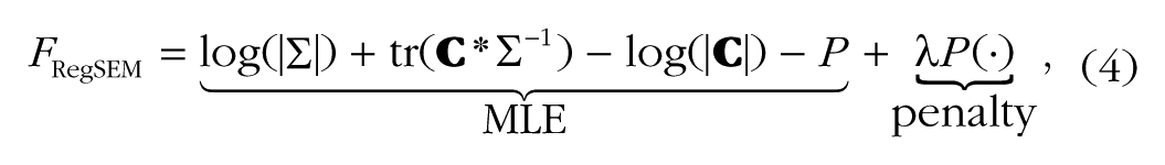
where
When the type of regularization is either the lasso or the elastic net (or another sparse penalty), the number of effective degrees of freedom can change as the penalty increases. Most notably, as the penalty increases, each parameter that is set to zero increases the degrees of freedom (see Jacobucci et al., 2016, for additional information). Thus, increasing the penalty often results in an improvement in fit as assessed by those fit indices that include the number of parameters in the equation (e.g., root mean square error of approximation, or RMSEA; comparative-fit index, or CFI; and information criteria). Note, however, that some fit indices are derived under the assumption that the point estimate is maximum likelihood; thus, it may be preferable to evaluate prediction error in a test set rather than to use classic in-sample test statistics (see Yarkoni & Westfall, 2017).
RegSEM combines confirmatory aspects of SEM with an exploratory search for important predictors. The confirmatory and exploratory aspects can take place in either the measurement or the structural parts of a structural equation model. In many situations, researchers may have some a priori idea of how some variables relate to each other. For instance, imagine that a group of researchers have constructed an initial CFA model with five indicators of a single latent variable, such as fluid intelligence. This confirmatory formulation may be based on previous research support for a single latent dimension underlying the covariance among the five indicators. Figure 2 displays the addition of three predictors (say, volumetric measures of different brain regions; cf. Kievit et al., 2014) to the initial CFA model. The resulting model is called a multiple-indicators (factor loadings), multiple-causes (regression parameters directed to the latent variable) model (MIMIC model; Jöreskog & Goldberger, 1975). Once the model is run, traditional techniques, such as the Wald test (and associated test statistics), can be used to determine which predictors have nonzero population values.
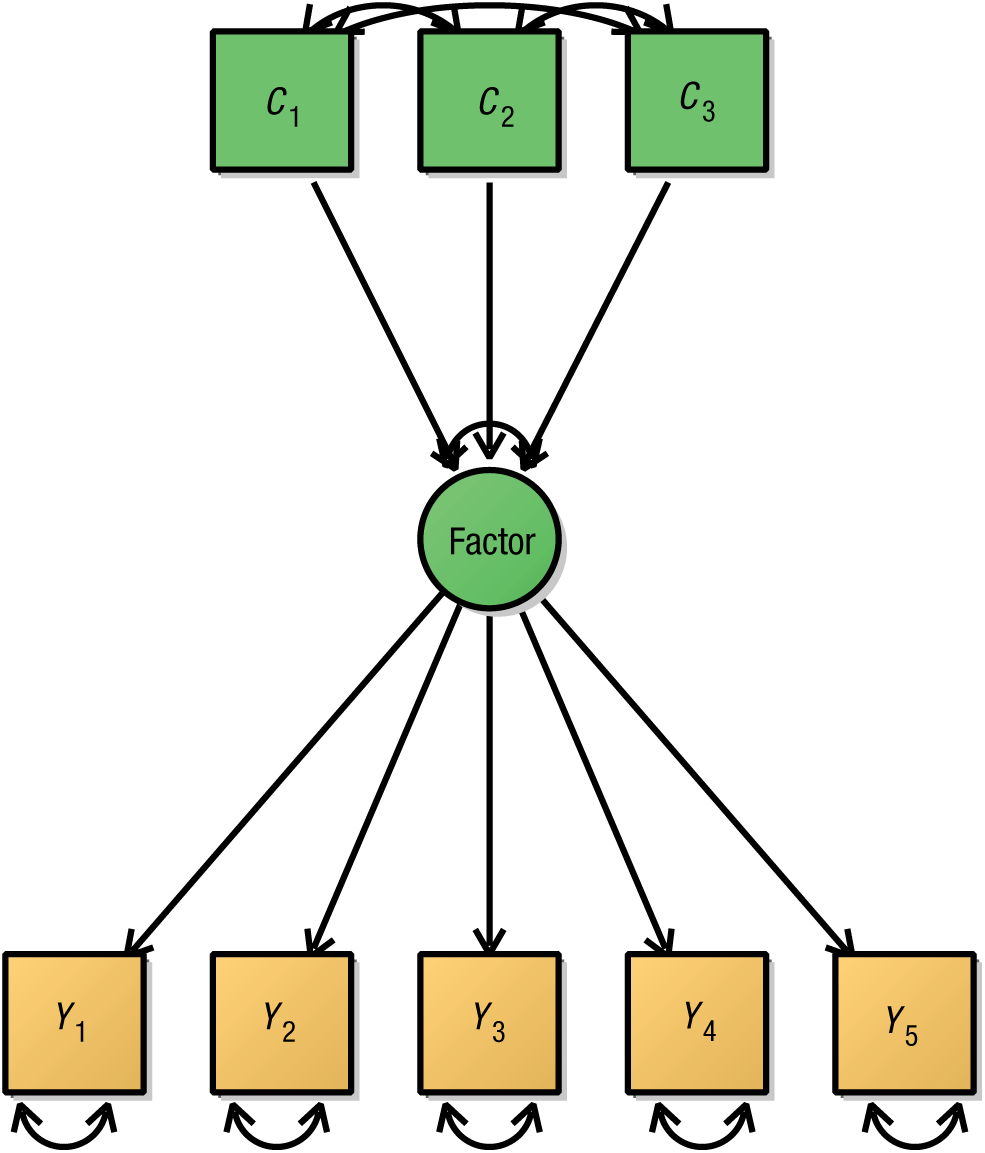
A simple multiple-indicators, multiple causes (MIMIC) model with five indicators (yellow boxes) and three predictors (green boxes) of a latent factor. Note that the variances of C1, C2, and C3 have been omitted.
This kind of model is commonly used to simultaneously estimate the joint influence of a set of presumed causal influences on one or more latent variables. However, given the constraints of traditional SEM approaches, the predictors are usually selected a priori on the basis of theoretical or empirical considerations (cf. Kievit et al., 2014). Now imagine an alternative scenario in which the researchers have a much larger number of predictors they wish to test (e.g., gray-matter volume in all regions identified in an atlas). None of these additional relationships may be based on previous hypotheses. The researchers may be relatively uncertain about which covariates in their data set are important predictors of the fluid-intelligence latent factor, either because they do not have strong a priori expectations or because there are a large number of candidates (e.g., genetic markers, brain variables). In this case, an exploratory search would be conducted. Traditional tools are no longer as suitable in such a scenario, as the model may not converge, or estimates may be imprecise, because of problems using MLE with large numbers of variables when the sample size is limited (e.g., see Hastie et al., 2015). Although previous research has examined the influence of large models on test statistics (Yuan, Yang, & Jiang, 2017), less attention has been paid to strategies that produce more accurate parameter estimates in large models. Here, in an effort to reduce this gap in the literature, we propose and evaluate the use of regularization.
In many applied fields such as genetics, cognitive neuroscience, and epidemiology, the ratio of predictors to the available sample size may be large. Indeed, one could argue that the absence of regularization methods may help explain why fields such as cognitive neuroscience rely on mass univariate approaches (i.e., a relationship between an outcome and neural data is tested thousands of times, separately for each brain region or voxel). However, multivariate approaches generally paint a richer, more realistic picture of the true data structure, and also allow the researcher to investigate which effects are redundant, and which may be partially independent and complementary. To examine the possible benefits of regularization in the SEM context, we conducted three studies. In Study 1, we examined the effectiveness of both MLE and regularization in the context of complex structural equation models. In Studies 2 and 3, we applied regularized SEM to large existing data sets.
Disclosures
The scripts for the simulation and applied analyses in this article are available online at https://osf.io/z2dtq/.
Study 1: Simulation
Method
To evaluate the effectiveness of the RegSEM lasso, we designed simulation conditions that researchers may commonly face when evaluating a large number of predictors (e.g., a property such as cortical thickness measured across many brain regions). We varied our simulations across two dimensions: sample size and predictor collinearity. The template model for our simulation is depicted in Figure 3. The model included six indicators (Y1–Y6) of the latent variable, f. The factor loadings of these indicators differed in their simulated population values (see Fig. 3). As predictors of f, there were 70 uninformative (noise) variables (Cn1–Cn70), with simulated population coefficients of zero. Additionally, there were three sets of 10 predictors each; a set of predictors with small effect sizes (0.20, Cs1–Cs10), a set of predictors with medium effect sizes (0.50; Cm1–Cm10), and a set of predictors with large effect sizes (0.80; Cl1–Cl10). Taken together, there were 100 potential predictors of f, each treated as a fixed effect. The variance of the latent variable was fixed to 1 for identification purposes, so that each factor loading could be freely estimated (we did not estimate a mean structure).
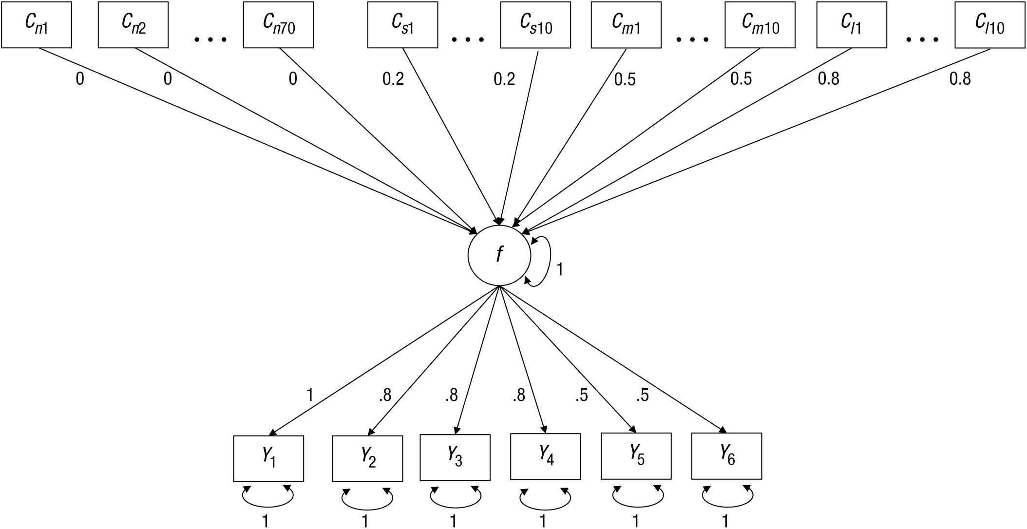
Template model for the simulation in Study 1. This multiple-indicators, multiple-causes (MIMIC) model included a single latent factor f, six indicators (Y1–Y6) with factor loadings from .5 to 1 and unique error variances, and 100 potential predictors. Some predictors were uninformative (Cn1–Cn70), and others had a small effect (Cs1–Cs10), a moderate effect (Cm1–Cm10), or a strong effect (Cl1–Cl10).
After creating simulated data according to the model in Figure 3, we tested a model that included 112 free parameters: 100 regression coefficients, 6 factor loadings, and 6 residual variances. Although rules of thumb are inherently limited, common guidelines suggest a ratio of 10:1 between sample size and the number of free parameters (e.g., Kline, 2015) to obtain stable estimates. In this case, that would mean a minimum N of 1,200. Given that many researchers may wish to test models of this size, but may not have the requisite sample size, we wanted to test a variety of sample sizes to examine when the performance of MLE degrades and when the use of regularization is beneficial. Therefore, we tested sample sizes 2 of 150, 250, 350, 500, 800, and 2,000.
In most psychological studies that examine the influence of a variety of predictors, these predictors have correlations among themselves. This complicates the interpretation of the results. For instance, it becomes challenging to determine the relative contribution of individual predictors (Grömping, 2009). Moreover, high degrees of collinearity can result in problematic estimation. Therefore, we also investigated the effect of predictor collinearity in our simulation by simulating data with correlations of 0, .20, .50, .80, and .95 among all predictors. We expected that bias in both MLE and regularized estimation would increase as the correlation among predictors increased. Because lasso regularization is problematic with high degrees of collinearity, we also tested the elastic-net estimator. Finally, we examined the prevalence of Type I errors (wrongly including a noise predictor in the final model) and Type II errors (wrongly excluding a true predictor) across the sample sizes and effect sizes.
To test each form of estimation, we used a different package in the R statistical environment (R Core Team, 2018). For MLE, we used the lavaan package (Version 0.5-23.1097; Rosseel, 2012). For RegSEM, we used the regsem package (Version 1.0.6; Jacobucci, Grimm, Brandmaier, & Serang, 2017). Both lasso and elastic-net regularization are implemented in regsem, along with a host of additional penalties (Jacobucci, 2017). We varied λ (see Equation 4) across 30 values, ranging from 0 to 0.29 in equal increments. In initial preruns, higher penalty values were included, but they always resulted in worse fit. To choose a final model among the 30 models run, we used the Bayesian information criterion (BIC; Schwarz, 1978). Each cell in the simulation’s design was replicated 200 times.
Results
Instead of giving a detailed analysis of the simulation’s results, we provide a high-level overview. We compare the performance of the RegSEM lasso with the performance of MLE using three metrics: root mean square error (RMSE; averaged across each set of parameters), relative bias (averaged across each set after taking the absolute value of each parameter), and error rate (for Type I and Type II errors, respectively). For each performance metric, we discuss how results varied across sample sizes and predictor collinearities. We do not present the results for RegSEM elastic-net estimation, as those results were almost identical to the results for the RegSEM lasso.
Parameter estimates
First we discuss the precision of parameter recovery, quantified as RMSE (Fig. 4) and relative bias (Fig. 5). At high sample sizes, the results for RMSE showed that MLE performed similarly to the lasso, and MLE’s performance was better than the lasso’s when performance was measured by relative bias. This difference in results for the two metrics was expected, because, as we discussed earlier, the lasso imparts bias to reduce variance. RMSE measures both bias and variance, whereas relative bias measures only bias; thus, with the lasso, the increase in bias is somewhat offset by a decrease in variance. At small sample sizes, and particularly a sample size of 150, the lasso performed better than MLE with regard to both RMSE and relative bias. In conditions with only 150 observations, MLE was highly unstable in its estimation of parameters; that is, parameter estimates were drastically larger than their simulated values.
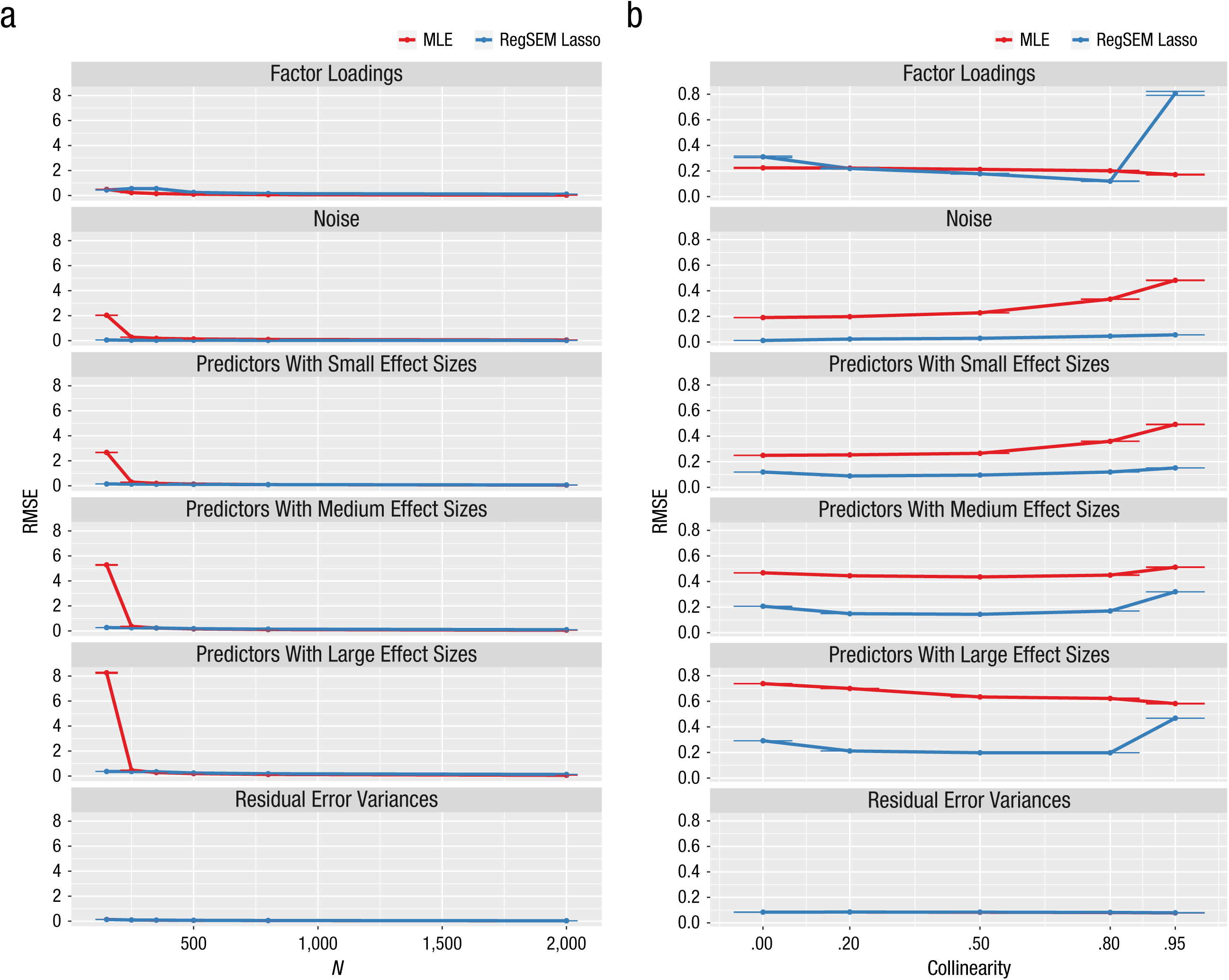
Results from Study 1: root mean square error (RMSE) as a function of (a) sample size and (b) predictor collinearity. Results are shown separately for maximum likelihood estimation (MLE) and the RegSEM lasso. From top to bottom, the graphs show results for the factor loadings, the uninformative predictors (noise), the informative predictors of different effect sizes (small, medium, and large), and the residual error variances. Error bars represent ±1 Monte Carlo standard error. Note that some of the error bars are barely visible because of very small values.
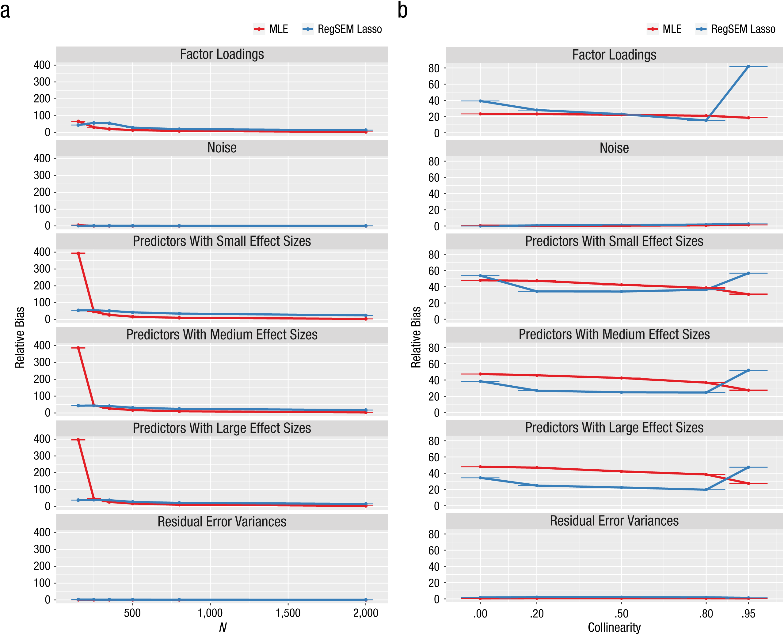
Results from Study 1: relative bias as a function of (a) sample size and (b) predictor collinearity. Results are shown separately for maximum likelihood estimation (MLE) and the RegSEM lasso. From top to bottom, the graphs show results for the factor loadings, the uninformative predictors (noise), the informative predictors of different effect sizes (small, medium, and large), and the residual error variances. Error bars represent ±1 Monte Carlo standard error. Note that some of the error bars are barely visible because of very small values.
The lasso produced better RMSE results than MLE in most conditions, particularly with sample sizes of 150 and 250. When the correlation among all predictors was extremely high (.95), the lasso produced a large amount of RMSE in the factor loadings. This condition is probably the reason why the RMSE values for the estimates of the factor loadings were higher for the lasso than for MLE across sample sizes. This poor performance can most likely be explained by covariance expectations and by the fact that correlations among predictors create a complicated web of relationships (see the appendix for further details). Fortunately, collinearity of predictors in the range of .95 is unlikely to be observed in real data sets.
The results for relative bias were more mixed. The lasso produced less relative bias than MLE for the sample size of 150, but MLE produced less relative bias with larger samples. An extreme degree of collinearity resulted in a large increase in relative bias for the lasso, much as extreme collinearity increased RMSE for the lasso. This secondary effect of collinearity was much less evident with MLE. Collinearity had a U-shaped effect on relative bias of the regression coefficients when the lasso was used: Both small (.00) and extreme (.95) correlations among predictors resulted in the highest relative bias. In contrast, this relationship did not hold for MLE. Together, our simulations show that regularized SEM outperforms traditional MLE in accuracy of parameter estimation when sample sizes are small and the number of predictors is large.
Type I and Type II errors
An alpha criterion of .05 was used to determine parameter significance in the MLE models. Thus, a Type I error occurred when the coefficient for a noise variable had a p value less than .05. Results for the frequency of Type I errors (see Fig. 6) showed that sample size had a larger effect than did collinearity in the MLE models. For a sample size of 150, there was a 17% chance for a noise variable to be incorrectly identified as a significant parameter. Although the Type I error rates were higher than .05 across the range of collinearities tested, this can mostly be attributed to the influence of sample size. A Type II error occurred when the coefficient for a predictor with a small, medium, or large simulated effect size had a p value greater than .05. Results for Type II errors (see Fig. 6) were alarming in that they indicated there was low power to detect the effects of the parameters with small and medium simulated effect sizes. As collinearity increased, so did the Type II error rates for these parameters (i.e., power decreased); the inverse relationship held for sample size. Even for the parameters with a simulated effect size of 0.8, larger-than-expected numbers of Type II errors were committed when sample sizes were small and when collinearity was high.
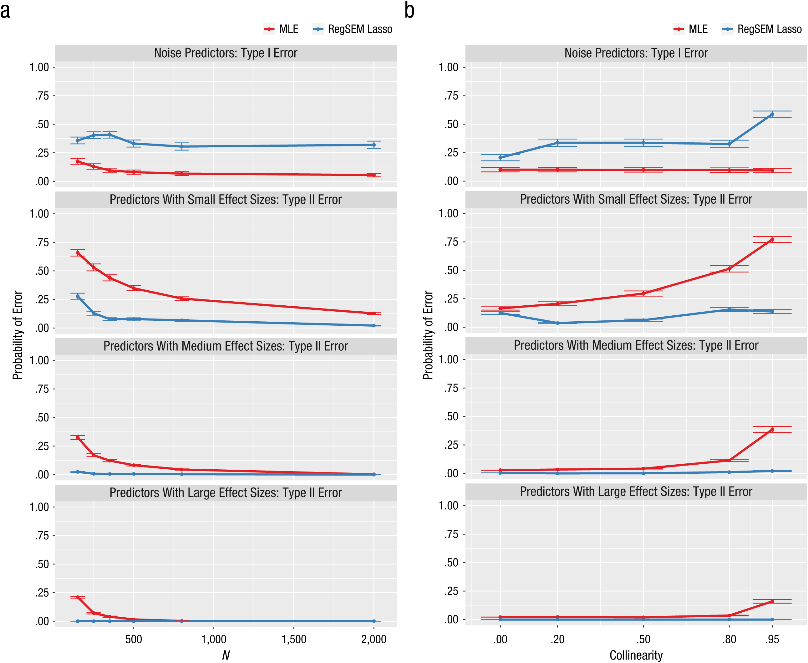
Results from Study 1: probability of committing Type I and Type II errors as a function of (a) sample size and (b) predictor collinearity. Results are shown separately for maximum likelihood estimation (MLE) and the RegSEM lasso. From top to bottom, the graphs show results for noise predictors and predictors with small, medium, and large effect sizes. Error bars represent ±1 Monte Carlo standard error. Note that some of the error bars are barely visible because of very small values.
Overall, the lasso models committed far more Type I errors than the MLE models, but also had much lower Type II error rates (i.e., they rarely omitted a truly predictive variable).
Summary
Across our simulations, the MLE models estimated parameters more accurately than the lasso models when sample sizes were large, and the lasso models were more accurate than the MLE models when sample sizes were small. Overall, the MLE models had less relative bias (as expected), but the lasso models improved upon the MLE models with respect to the RMSE. The RegSEM lasso committed more Type I errors then MLE did, but achieved much higher rates of power (lower Type II error rates) across conditions. These results are in line with previous findings, such as those of Serang, Jacobucci, Brimhall, and Grimm (2017), who found a similar trade-off between regularization and other forms of estimation in the context of mediation models. The optimal method for a given research context depends on the relative importance of decreasing parameter bias and decreasing parameter variance. Within a given sample, an MLE model may produce more accurate results than a model using regularization, but the MLE model may not generalize as well. We note that the contrast between these forms of estimation may not apply beyond the small selection of models we discuss here.
Study 2: White-Matter Determinants of Visual Short-Term Memory
Many features of brain structure and function may have complementary cognitive effects. Thus, a challenge in cognitive neuroscience is how to reconcile the dimensionality constraints of covariance-based methodologies such as SEM with the richness of the imaging metrics (which may include hundreds of measures per individual). Here, we describe an illustrative example in which we used regularized SEM to model visual short-term memory (VSTM) as a function of white-matter microstructure. The data came from the Cambridge Study of Cognition, Aging and Neuroscience (Cam-CAN, www.cam-can.org; Shafto et al., 2014), a study of a large, population-derived cohort of healthy individuals
The Sample
The data for this empirical illustration are from 627 adults (320 female; age range from 18 to 88, M = 54.18, SD = 18.42) who participated in a large battery of cognitive tests, demographic and life-style measurements, and MRI scans (for more details on the cohort and sampling methodology, see Taylor et al., 2017). We focus on participants who had complete data for a specific cognitive task (the VSTM task) and a common index of white-matter microstructure (fractional anisotropy). Analyses of subsets of these MRI data (but not the data for this cognitive task) have previously been reported (e.g., Henson et al., 2016; Kievit et al., 2016; Kievit et al., 2014).
The VSTM task
The VSTM task in the Cam-CAN battery was developed to quantify the capacity and precision of VSTM. The task consists of three phases: an encoding phase, during which participants view one to four colored circles (targets); a brief blank screen (900 ms); and a cue in the same spatial location as one of the target circles (see Fig. 7). Participants are asked to use a color wheel to pick the color of the circle that previously appeared at the cued location, as well as to rate their confidence in their judgment. They performed a total of 224 trials across two blocks; position of the targets, set size, and cue (i.e., which target was cued) were counterbalanced across blocks. We focus here on the effects of set size for set sizes 2 through 4 (to avoid the ceiling effects associated with the simplest version of the task). Each participant’s mean performance for each of these three set sizes was scored; the scores for each set size ranged between 0 and the maximum number of circles for that set size.
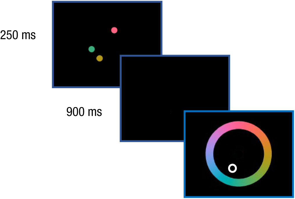
The visual short-term memory task in the Cambridge Study of Cognition, Aging and Neuroscience (Shafto et al., 2014). On each trial, participants viewed from one to four target circles for 250 ms and then a 900-ms blank screen. Finally, a cue for one of the previous targets was presented, and participants were asked to use a color wheel to indicate which hue most closely matched that of the cued target.
White-matter predictors
For the neural indicators, we used a common metric of white-matter organization called fractional anisotropy. This metric quantifies the dispersion of water molecules and the extent to which this dispersion is constrained by the organization of white-matter structures. Fractional anisotropy is a complex and indirect measure with various limitations, and its relationship to white-matter health is not yet fully understood (Bender, Prindle, Brandmaier, & Raz, 2016; Jones, Knösche, & Turner, 2013). Nonetheless, fractional anisotropy is widely used, as it has been shown to be associated with individual differences in a range of cognitive domains, especially in old age (Madden et al., 2009). We focused on mean fractional anisotropy for each tract in the ICBM-DTI-81 atlas (Mori et al., 2008), which parcellates the human white-matter skeleton into 48 tracts. Although our previous work used white-matter atlases of lower dimensionality (e.g., Kievit et al., 2016, and de Mooij, Henson, Waldorp, & Kievit, 2018), we intentionally used a more high-dimensional white-matter atlas for this example to illustrate the benefit of regularization. (For more details regarding the analysis pipeline, see Kievit et al., 2016.)
The MIMIC model
To examine the neural determinants of VSTM, we fit a MIMIC model (Jöreskog & Goldberger, 1975). Our model captured the hypothesis that VSTM (the latent variable), which was measured by scores on the VSTM task (the multiple indicators), was in turn affected by the fractional anisotropy of various white-matter tracts (the multiple causes; see Kievit et al., 2012, for a comparison of the MIMIC model with competing representations). First, we specified a measurement model in which the latent VSTM variable was measured by memory scores at each of the three set sizes (2, 3 and 4). Next, we simultaneously regressed this latent variable on the fractional anisotropy for all 48 white-matter tracts. This model tested the joint prediction of the latent variable by all 48 white-matter tracts, which allowed us to determine whether one or more tracts helped predict individual differences in VSTM.
Model estimation and results
We estimated the regularized model across a range of λ values and used the BIC (also known as the Schwarz criterion) to compare the fit of these models (see Jacobucci, Grimm, & McArdle, 2016, for details on alternative strategies for selecting a final model). The BIC balances the increased parsimony achieved by regularizing parameters to zero with the concurrent decrease in explanatory power. As we had a strong a priori hypothesis about the measurement model, we regularized the structural parameters (i.e., the joint prediction of the latent variable by the 48 tracts), but not the factor loadings or residual variances. As Figure 8 shows, the best solution was obtained with a λ value of 0.18. This model yielded an acceptable RMSEA of 0.0321. Figure 9 shows the beta estimates across a range of λ values, as well as the location of the 6 tracts with nonzero beta estimates in the final model.
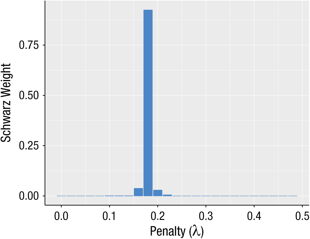
Results from Study 2: Schwarz weights (cf. Wagenmakers & Farrell, 2004) of the models as a function of the penalty (λ) value. Higher weights correspond to lower values of the Bayesian information criterion and thus indicate a better-fitting model.
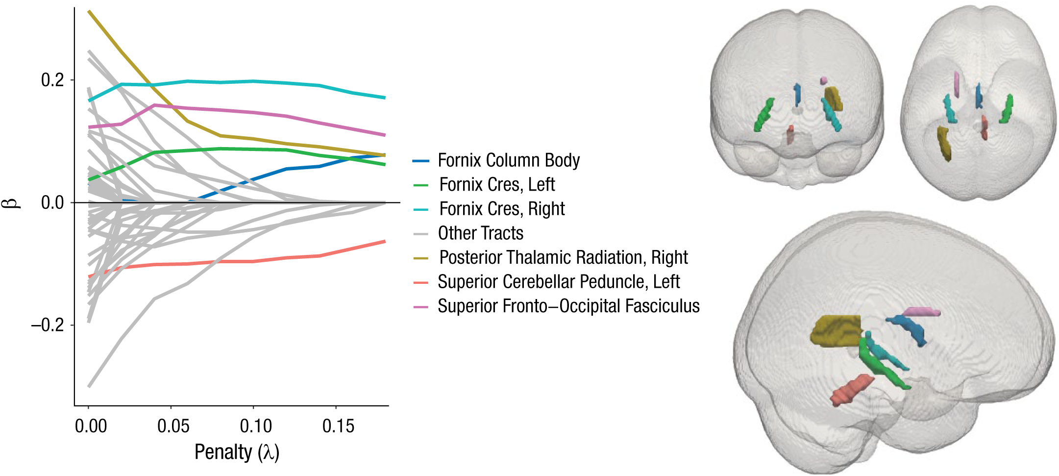
Results from Study 2: beta estimates for the white-matter tracts as a function of the penalty (λ) value and brain maps showing the location of the six tracts with nonzero estimates in the final model. Note that the tracts with effects regularized to zero are shown in gray.
As Figure 9 shows, the beta estimates for six tracts remained nonzero in the regularized MIMIC model. Strikingly, three of these tracts are subdivisions of the fornix (the column body, as well as the cres), and all showed positive effects (i.e., greater white-matter microstructure was associated with better VSTM performance). The fornix, which connects the hippocampus to other brain regions, has long been associated with various aspects of memory, usually autobiographic memory (e.g., Hodgetts et al., 2017) but also, in the Cam-CAN cohort, subdomains such as recollection, familiarity, and priming (Henson et al., 2016). Notably, there have been some Phase I trials suggesting that deep-brain stimulation to the fornix may alleviate memory complaints in patients with early Alzheimer’s disease (Laxton et al., 2010). The posterior thalamic radiations (see Fig. 9) have been posited as crucial for focusing and allocating attention in demanding tasks (Menegaux et al., 2017). Evidence from infants suggests an association between greater white-matter organization in the posterior thalamic radiations and better performance on the VSTM task (Menegaux et al., 2017). Finally, we observed a positive association between VSTM performance and white-matter microstructure of the superior fronto-occipital fasciculus, which was positively associated with children’s spatial working memory in previous research (Vestergaard et al., 2011).
Although the results for these five tracts align well with previous literature, we also observed a single (surprising) negative effect: Greater white-matter integrity of the superior cerebellar peduncle was associated with poorer VSTM performance. However, closer inspection suggested that this pattern was likely an artifact of image registration, as the integrity of this tract, unlike others, increases (bilaterally) with age. A likely explanation is that the relatively deep location of this tract within the brain makes it vulnerable to registration challenges, such as partial volume effects (Alexander, Hasan, Lazar, Tsuruda, & Parker, 2001). We suggest that this negative pattern is more likely due to an imaging artifact than to a true association.
It should be noted that the regularized model solution does not imply that the white-matter microstructure of all the other tracts is uncorrelated to VSTM. When predictors are collinear, the predictors that emerge in a regularized solution are likely to be the most representative of broader sets of correlated predictors (in the present case, a single tract may capture most or all of the predictive power across a network of tracts). In the case of collinear predictors, regularizing groups of predictors with the group lasso (Friedman, Hastie, & Tibshirani, 2010) may be more appropriate than regularizing individual predictors; however, this approach has not yet been generalized to SEM.
To summarize, a regularized structural equation/MIMIC model was able to model the relation between cognitive performance and imaging metrics, taking a high-dimensional set of predictors and reducing this set to create a relatively parsimonious representation of key tracts previously implicated in VSTM performance. These results demonstrate the viability of this methodology in cognitive neuroscience in general and in research with aging and developmental cohorts in particular.
Study 3: Modeling the Determinants of Depression, Anxiety, and Stress
The Sample
Previous work has suggested that there are many distinct predictors of individual differences in depression, anxiety, and stress (e.g., Sümer, Poyrazli, & Grahame, 2008), but the extent to which these determinants of mental health are separable or collinear (nonunique) is unclear. For our second empirical example, we attempted to answer this question using a large (N = 27,835) publicly available data set containing answers to the Depression Anxiety Stress Scales (DASS; Lovibond & Lovibond, 1995). This data set was collected from an online sample and is freely available at https://openpsychometrics.org/_rawdata/. The 42-item DASS captures latent variables of depression, anxiety, and stress (each with 14 indicators), and the data set also includes a set of personality and demographic covariates, which we subjected to regularization. These covariates include responses on the Ten-Item Personality inventory (TIPI; Gosling, Rentfrow, & Swann, 2003), which uses 7-point Likert scales (from disagree strongly to agree strongly). Other covariates are highest level of education (ranging from 1, less than high school, to 4, graduate degree), gender (1 = male, 2 = female), age (in years), handedness (1 = right, 2 = left), voter record (1 = I have voted in the last year, 2 = I have not voted in the last year), and family size (“Including you, how many children did your mother have”; participants filled in the correct number). These covariates are included for illustrative, rather than conceptual, reasons.
Results
First, we fit a three-factor measurement model to all the DASS data. This model fit the data well, χ2(816) = 64,490.79, p < .001; RMSEA = 0.053, 90% confidence interval = [0.053, 0.053]; CFI = 0.897; standardized root mean square residual = .040, and all factor loadings were moderate to strong (range = .50–.84, M = .70). Despite considerable covariance among the latent variables (all correlations > .7), a three-factor model fit considerably better than a competing unidimensional account (in which all items were taken to measure a single latent variable), Δχ2 = 29,414, Δdf = 3, p < .001. Next, we fit a MIMIC model in which the three latent factors were simultaneously regressed on the 16 predictors. Results reported here are based on a random subsample (N = 1,000) of the full cohort. Model fit was good, χ2(1440) = 4,348.61, p < .001; RMSEA = 0.045, 90% confidence interval = [0.044, 0.046]; CFI = 0.884; standardized root mean square residual = .038, and the joint covariates predicted a large amount of variance (depression: 40.7%; anxiety: 41.9%; stress: 52.3%). In this same subsample, MLE yielded 4 predictors that were nominally significant for stress, 7 that were significant for anxiety, and 6 that were significant for depression (see Fig. 10).
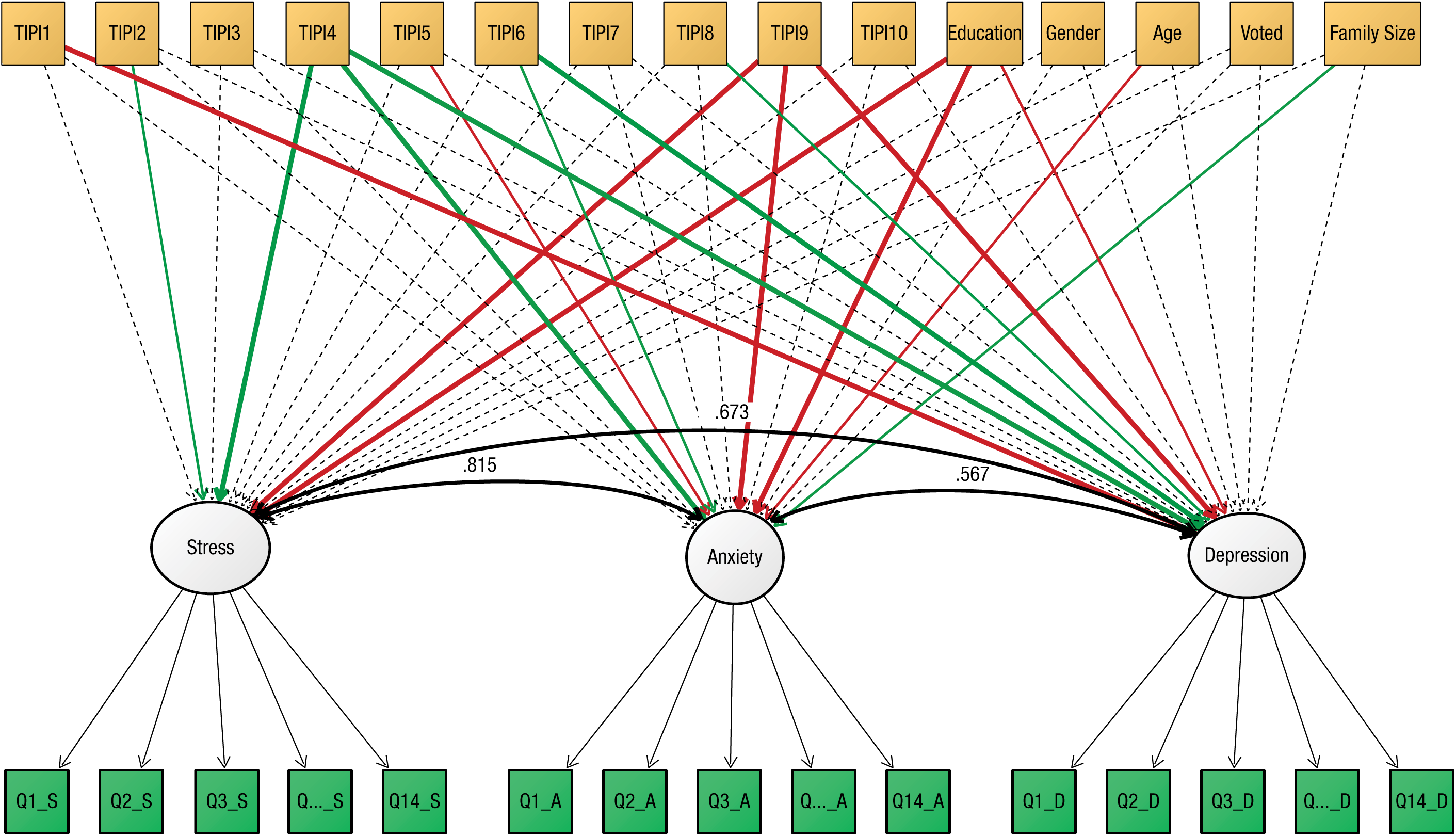
Results from Study 3: multiple-indicators, multiple-causes (MIMIC) model of stress, anxiety, and depression. Dashed lines indicate nonsignificant paths, and solid lines indicate significant paths (α < .05) in the maximum likelihood model. The color of the solid lines indicates whether effects are positive (green) or negative (red), and the lines’ thickness indicates the strength of the effects (thick = z > 3, thin = z < 3). TIPI1 through TIPI10 refer to the items on the Ten-Item Personality inventory (Gosling, Rentfrow, & Swann, 2003). Q1_S through Q14_D (in the green boxes) refer to the items on the Depression Anxiety Stress Scales (Lovibond & Lovibond, 1995). For purposes of clarity, results for the handedness predictor are not shown. Variances are omitted from this figure.
Next, we refit the model using the RegSEM lasso. Forty penalty values were tested, and Figure 11 summarizes the results. The optimal BIC solution was observed with a λ value of 0.15. This penalty regularized the paths of 27 of the 48 structural parameters to zero, yielding the most parsimonious model representation. Table 1 shows the fully standardized parameter estimates for the MLE model as well as the regularized model. Across all three factors, two TIPI items—4 (“easily upset, anxious”) and 9 (“calm, emotionally stable”)—had strong associations (r = ~.3) with the three mental-health outcomes. Note that the strong associations between the latent factor anxiety and TIPI Item 4 is unsurprising given their partial content overlap. However, both the MLE and the lasso estimates demonstrate that a considerable number of additional predictors, including education and “reserved, quiet” (TIPI Item 6) personality, explained unique variance in individual differences in mental health. Moreover, the DASS and TIPI purportedly capture distinct domains (mental health and personality), and this model is meant for illustrative purposes only. We present these parameters for readers to interpret accordingly.
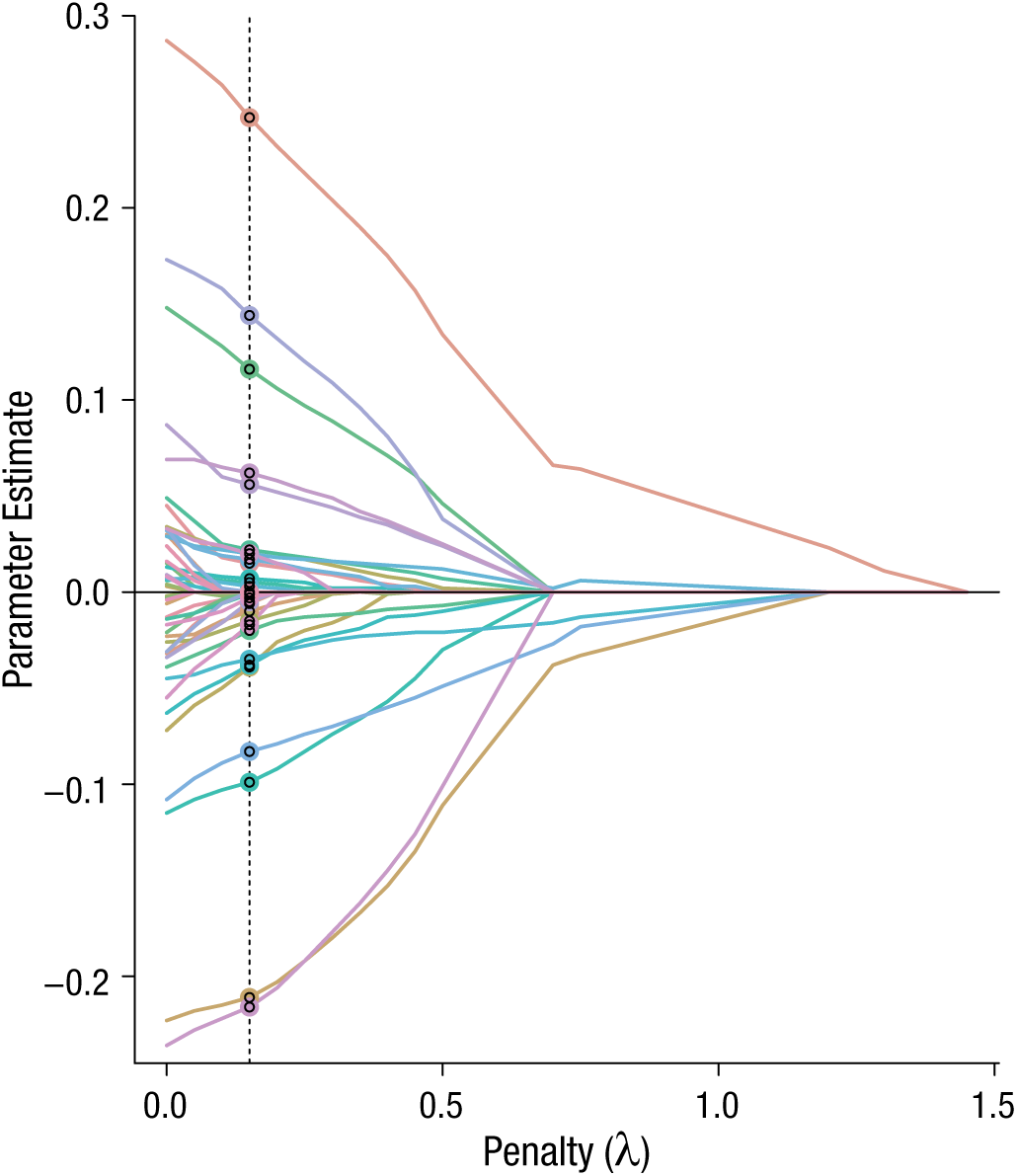
Parameter trajectory plot from Study 3. The graph shows the values of the 48 regression coefficients as a function of the penalty value. The dashed vertical line highlights the penalty value yielding the model with the best fit (i.e., the lowest Bayesian information criterion).
Results From Study 3: Fully Standardized Regression Parameters From the Maximum Likelihood and Lasso Models
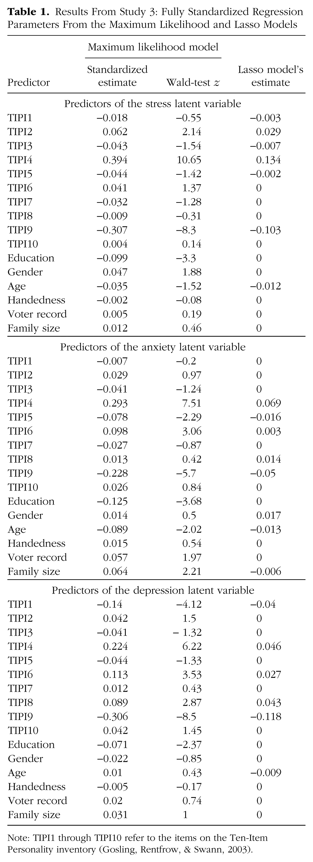
Note: TIPI1 through TIPI10 refer to the items on the Ten-Item Personality inventory (Gosling, Rentfrow, & Swann, 2003).
Note that the predictors with the largest Wald-test z values in Table 1 do not consistently correspond to the predictors selected as having nonzero coefficients in the lasso model. One thing to keep in mind when interpreting lasso parameter estimates is that they are biased toward zero because of the shrinkage (Tibshirani, 1996). To address this bias, one can refit the model without any penalty in a second stage that includes only the chosen subset of predictors. This procedure, which is referred to as the relaxed lasso (Meinshausen, 2007), has been shown to perform favorably compared with best-subset selection, forward stepwise selection, and the lasso without the second stage (Hastie, Tibshirani, & Tibshirani, 2017; Serang et al., 2017). Because we did not follow this two-stage approach, the regularized coefficients are best interpreted only as zero or nonzero.
Discussion
We have argued that regularized SEM is a powerful and underutilized method for researchers who want to examine a (relatively) large number of predictors, or who have a relatively modest sample size combined with a model of moderate complexity. We have described regularization as applied to both regression and SEM, and have evaluated its use in high-dimensional MIMIC models. In our simulation study, models with lasso penalties incurred less error than MLE models when sample sizes were small and demonstrated higher power to detect effects of small and medium magnitude. Our results illustrate how sample size and the correlation among regressors influence the accuracy of parameter estimates and how variable selection is performed in an extremely complex model. Regularized SEM was applied to modeling VSTM as a function of white-matter microstructure in a large existing data set. Starting with a complex model of 48 distinct white-matter tracts, the regularized model identified 6 tracts as determinants of VSTM. Finally, in our last example, we used a regularized model to identify a broad set of variables that explain individual differences in stress, anxiety, and depression.
Our simulation study showed that regularized SEM may be a viable option for researchers looking to identify relatively low-dimensional sets of predictors in fields with broad sets of candidate variables, such as cognitive neuroscience and behavior genetics. Notably, this technique goes beyond traditional methods used to correct for multiple comparisons in neuroimaging studies. Methods that correct for multiple comparisons, such as those based on the false discovery rate and Gaussian random-field theory (for an accessible introduction, see Brett, Penny, & Kiebel, 2003), are generally still implemented to correct (mass) univariate tests, rather than joint simultaneous prediction across voxels (regions of interest). It may be possible to combine regularized SEM with methods of joint comparisons, such as principal component regression, to estimate the joint predictive value of multiple components across many voxels even in cases with modest sample sizes (e.g., Wager, Atlas, Leotti, & Rilling, 2011).
Limitations and challenges
Although we have illustrated several benefits of regularization in regression and SEM when sample sizes are small, we did not include any conditions with sample sizes below 100 in our simulation study. This was mostly due to the complexity of our model, as we were unable to achieve stable estimates at a sample size of 120 or below. In regularized regression, it is possible to test models in which there are more predictors than observations; however, to our knowledge, methods of testing models with more predictors than observations have not been extended to SEM, and we were unsuccessful in our attempt to apply regularized SEM to such cases in our simulation study. A possible solution is to use Bayesian SEM, in which strongly informative priors or hierarchal models with sparsity-inducing priors can achieve stable estimation even in such extreme cases (see Jacobucci & Grimm, 2018). Given that Bayesian estimation is increasingly being used in cases of small numbers of observations (McNeish, 2016), and that pairing of Bayesian SEM and regularization has been more widely applied than pairing of frequentist SEM and regularization (see Brandt, Cambria, & Kelava, 2018; Feng, Wu, & Song, 2017; Lu, Chow, & Loken, 2016), we expect to see more research in this area in the future. Other avenues for future work include investigating bias when regularization is used in factor-score regression (Devlieger & Rosseel, 2017), a method that may help overcome the current limitation of needing more observations than predictors. Additionally, bias induced by high degrees of collinearity may be reduced by first creating factor scores, and thus fixing the factor loadings.
Frequentist software for regularized SEM currently requires complete cases. As it is rare for psychological data to have no missing values, this requirement is currently a considerable weakness of regularized SEM. One strategy for modeling data with missing values is multiple imputation. The main issue with using this strategy with regularized SEM concerns how to combine the results. In traditional multiple imputation for SEM, parameter estimates can be aggregated across 10 to 20 data sets (or more) by averaging the parameter estimates and correcting the standard errors for the lack of randomness in the process. However, regularization is most often used to perform variable selection, and this necessitates a way to aggregate a set of 0 to 1 decisions across imputed data sets. Although some research has addressed how to aggregate results in regression (Liu, Wang, Feng, & Wall, 2016), this work has not been generalized to SEM.
Lockhart, Taylor, Tibshirani, and Tibshirani (2014) have derived sampling distributions to calculate p values that take into account the adaptive nature of the lasso regression model, but this work has not been extended to SEM with the lasso. When parameter estimates are not accompanied by p values or confidence intervals, researchers may feel uncertain in making inferences. Consequently, inference can be more challenging with regularized structural equation models than with regularized regression models, particularly given the inherent bias in estimation. One proposed method for overcoming this challenge is the relaxed lasso (Meinshausen, 2007), which has been shown to produce unbiased parameter estimates when applied to mediation models (Serang et al., 2017).
It may be difficult to change the mind-set of relying on p values and instead to characterize nonzero paths as important. To overcome this difficulty, we recommend thinking in terms of generalizing to an alternative sample. Although researchers may incur bias when using regularization, the more important aim is generalization, which is achieved by reducing variance and preferring models of a complexity that is afforded by the observed data. This holds true particularly for exploratory studies, which are less concerned with within-sample inference and more concerned with informing future research.
In our simulation, we found a trade-off between MLE and the RegSEM lasso with respect to Type I and Type II errors: The RegSEM lasso kept more variables in the model (more Type I and fewer Type II errors), whereas MLE was more restrictive with respect to which variables were deemed significant (fewer Type I and more Type II errors). In exploratory studies, we generally recommend a liberal stance; that is, more emphasis should be given to the inclusion of potentially important variables, and the possibility of including variables that do not have either predictive or inferential value should be of less concern. In an ideal setting, researchers would apply regularized SEM to data from a pilot or initial study in the hopes of being maximally efficient in identifying what variables should be included in a future, possibly larger study. Our simulation study supports the idea that applying MLE when the sample is small and the number of variables is large will result in the exclusion of potentially relevant variables. Note, however, that our conclusions depended not only on the method of regularization applied but also on the specific heuristic for choosing the penalty (i.e., relying on fit indices rather than domain expertise). The penalty values that align with the goals of researchers who want to be relatively inclusive in variable selection (i.e., who can tolerate more Type I errors) may be different from the penalty values that align with the goals of researchers who want to be more exclusive (i.e., who can tolerate more Type II errors; (see also Lakens et al., 2018).
Related approaches
Regularized SEM is only one of the new methods developed for SEM with large data sets. Particularly in the area of variable selection, SEM trees (Brandmaier, von Oertzen, McArdle, & Lindenberger, 2013) and forests (Brandmaier, Prindle, McArdle, & Lindenberger, 2016) are alternative methods. SEM trees directly use the observed covariates to partition observations, and in the process, only a subset of covariates are used to create the model. This allows researchers to uncover nonlinearities and interactions. Additional methods include the use of heuristic search algorithms (e.g., Marcoulides & Ing, 2012), various methods for identifying group differences (Frick, Strobl, & Zeileis, 2015; Kim & von Oertzen, 2018; Tutz & Schauberger, 2015), and the use of graphical models for identifying latent variables (e.g., Epskamp et al., 2017). Given the increasing amounts of data sharing, facilitated by various new tools for data storage and sharing, such as the Open Science Framework (https://osf.io/) and OpenfMRI (https://openfmri.org/), we can envision the utility of testing models much larger than our template simulation model. One of the biggest challenges to such work is software implementation. In this regard, we expect Bayesian estimation (see Jacobucci & Grimm, 2018), discussed earlier, to be a particularly fruitful alternative to our frequentist approach, especially in the creation of new sampling methods such as those in the Stan software package (Carpenter et al., 2016). Interfaces for specifying models (see Merkle & Rosseel, 2015) are sure to be more widely used among psychological researchers as they become easier to use.
Concluding thoughts
We encourage researchers to think of regularization as an approach that can combine confirmatory and exploratory modeling. Regularization gives researchers more flexibility to make both their uncertainty and their knowledge concrete. It is particularly suitable when researchers hope to use a principled approach to go beyond the limitations of their theory to identify potentially fruitful avenues for future study. In both our simulation and our empirical examples, we conducted exploratory searches for important predictors in relation to a confirmatory latent-variable model. This is only one example of how these types of modeling can be fused, and we look forward to seeing new areas of application. We hope that this article sheds light on a new family of statistical methods that have much utility for psychological research.
Supplemental Material
JacobucciOpenPracticesDisclosure – Supplemental material for A Practical Guide to Variable Selection in Structural Equation Modeling by Using Regularized Multiple-Indicators, Multiple-Causes Models
Supplemental material, JacobucciOpenPracticesDisclosure for A Practical Guide to Variable Selection in Structural Equation Modeling by Using Regularized Multiple-Indicators, Multiple-Causes Models by Ross Jacobucci, Andreas M. Brandmaier and Rogier A. Kievit in Advances in Methods and Practices in Psychological Science
Footnotes
Appendix: Dependency Among Parameters in MIMIC Models
With two predictors (y1 and y2), and just one indicator (x1) of a single latent variable, the covariance between x1 and y1 (covx1,y1) is
where λx1 is the factor loading for x1, βy1 is the regression coefficient for y1, σy1 is the variance of y1, and σy1,y2 is the covariance between y1 and y2.
This equation means that when predictor covariance is high, the estimation of the second regression coefficient plays a large role. Thus, whenever parameters are overpenalized (either because the sample is not large enough to estimate them or because sparsity is desired), this bias not only is incurred in the regression, but also trickles down to the factor loadings. This is always a problem, as the model will try to “make up for” the downward bias of βy1 in the value assigned to λx1, but it can be exacerbated to a large extent when there is covariance among predictors. Adding in a large numbers of predictors makes the problem much worse.
Action Editor
Jennifer L. Tackett served as action editor for this article.
Author Contributions
R. Jacobucci, A. M. Brandmaier, and R. A. Kievit generated the idea for the studies and developed the simulation specification. R. Jacobucci ran the analyses. All three authors analyzed the results, generated the figures, and wrote the manuscript. All the authors approved the final submitted version of the manuscript.
Declaration of Conflicting Interests
The author(s) declared that there were no conflicts of interest with respect to the authorship or the publication of this article.
Funding
R. A. Kievit is supported by the Sir Henry Wellcome Trust (Grant 107392/Z/15/Z) and by an MRC Programme Grant (SUAG/014/RG91365). This project has also received funding from the European Union’s Horizon 2020 Research and Innovation program (Grant 732592).
Open Practices
All materials have been made publicly available via the Open Science Framework and can be accessed at https://osf.io/z2dtq/. The complete Open Practices Disclosure for this article can be found at http://journals.sagepub.com/doi/suppl/10.1177/2515245919826527. This article has received the badge for Open Materials. More information about the Open Practices badges can be found at ![]() .
.
Notes
References
Supplementary Material
Please find the following supplemental material available below.
For Open Access articles published under a Creative Commons License, all supplemental material carries the same license as the article it is associated with.
For non-Open Access articles published, all supplemental material carries a non-exclusive license, and permission requests for re-use of supplemental material or any part of supplemental material shall be sent directly to the copyright owner as specified in the copyright notice associated with the article.