On the Interpretation of Parameters in Multivariate Multilevel Models Across Different Combinations of Model Specification and Estimation

Abstract

The increasing availability of software with which to estimate multivariate multilevel models (also called multilevel structural equation models) makes it easier than ever before to leverage these powerful techniques to answer research questions at multiple levels of analysis simultaneously. However, interpretation can be tricky given that different choices for centering model predictors can lead to different versions of what appear to be the same parameters; this is especially the case when the predictors are latent variables created through model-estimated variance components. A further complication is a recent change to Mplus (Version 8.1), a popular software program for estimating multivariate multilevel models, in which the selection of Bayesian estimation instead of maximum likelihood results in different lower-level predictors when random slopes are requested. This article provides a detailed explication of how the parameters of multilevel models differ as a function of the analyst’s decisions regarding centering and the form of lower-level predictors (i.e., observed or latent), the method of estimation, and the variant of program syntax used. After explaining how different methods of centering lower-level observed predictor variables result in different higher-level effects within univariate multilevel models, this article uses simulated data to demonstrate how these same concepts apply in specifying multivariate multilevel models with latent lower-level predictor variables. Complete data, input, and output files for all of the example models have been made available online to further aid readers in accurately translating these central tenets of multivariate multilevel modeling into practice.

Multilevel models (MLMs)—also known as hierarchical linear models or linear mixed-effects models—are a mainstay of many areas of research. Their defining feature is their capacity to quantify and predict the sources of random variance that arise from sampling over multiple dimensions, such as across occasions, persons, or groups. For example, in a longitudinal design, one might examine how outcomes at different occasions (at Level 1) that are nested in different persons (at Level 2) can be predicted by time-varying or time-invariant characteristics (measured per occasion or per person, respectively). Likewise, in a clustered design, one might examine how outcomes for different persons (at Level 1) who are nested in different groups (at Level 2) can be predicted by person or group characteristics. Outcomes from even more complex designs can be analyzed by introducing additional random variances to reflect other sources of nested or crossed sampling. For ease of exposition (but without loss of generality), the focus in this article is limited to two-level models for nested samples.

The oldest (and still popular) MLM software packages estimate univariate multilevel models: They partition variance across levels of sampling for Level 1 outcomes. Examples of such software include the MIXED routines in SAS (SAS Institute, 2017), SPSS (IBM Corp., 2017), and Stata (StataCorp, 2017); the dedicated programs HLM (Raudenbush, Bryk, Cheong, & Congdon, 2011) and MLwiN (Charlton, Rasbash, Browne, Healy, & Cameron, 2019); and the R packages lme4 (Bates, Mächler, Bolker, & Walker, 2015) and nlme (Pinheiro, Bates, DebRoy, Sarkar, & R Core Team, 2019). As I elaborate later, the drawback of univariate MLMs is that an analogous model-based variance partitioning is not possible for Level 1 predictors (i.e., variables that relate to Level 1 outcomes via fixed effects instead of covariances). Instead, variance partitioning for a Level 1 predictor requires creating a new observed variable (i.e., a Level 2 mean over Level 1 units) to distinguish the unique effects of its Level 1 source of variance from its Level 2 sources of variance.

Fortunately, recent software advances have made it easier than ever before to estimate multivariate MLMs, in which variance is partitioned in both Level 1 predictors and Level 1 outcomes. Multivariate MLMs are estimable as multilevel structural equation models (SEMs) in Mplus (Muthén & Muthén, 2018), in gsem within Stata, and in the R package xxM (Mehta, 2013). To a more limited extent, multivariate MLMs can also be estimated as single-level SEMs, such as in LISREL (Jöreskog, Olsson, & Wallentin, 2016), Amos (Arbuckle, 2014), EQS (Bentler, 2008), sem within Stata, and lavaan (Rosseel, 2012) within R. However, their advantages in flexibility may come at the cost of more frequent user misunderstandings, given that the data transformations analysts use to create observed predictor variables in univariate MLMs may or may not be done behind the scenes through model-based variance partitioning (i.e., latent centering), depending on the multivariate MLM specification. Posing an additional challenge, the 2018 releases of Mplus (8.1 in June, 8.2 in November; Muthén & Muthén, 2018) have altered how the same multivariate MLM syntax gets implemented in multilevel SEMs—and thus how the results should be interpreted—when Bayesian estimation is selected instead of maximum likelihood (ML). As a result, analysts now have new considerations to address—and new sources of accidental error to avoid—in tackling the increasingly challenging intersection of research questions, models, and software.

My goal in this article is to help analysts avoid some common mistakes that can impede a meaningful multilevel analysis. First, I reinforce the importance of distinguishing the effects of predictors at different levels of analysis when specifying MLMs. To that end, I next use text, equations, and diagrams to review the terminology involved in creating and interpreting level-specific effects of observed predictor variables in univariate MLMs. Fortunately, this first section is applicable to univariate MLMs estimated using any software package; I have provided corresponding univariate MLM examples using Mplus in the Supplemental Material available online, but analogous examples can be found in many online sources (e.g., Hoffman, 2018; UCLA Institute for Digital Research & Education, 2019).

Second, I demonstrate how to interpret parameters from multivariate MLMs specifically, for which understanding the (ever-changing) ties between model specification and software implementation is even more critical. I provide examples of multivariate MLM results obtained through two different software frameworks: (a) multilevel structural equation modeling in Mplus specifically and (b) single-level structural equation modeling (as implemented in any SEM software that allows random slopes, including Mplus). Using simulated data, equations, and figures, I show how the concepts presented for univariate MLMs still apply to specifying and estimating multivariate MLMs. To aid readers in translating these examples into analyses of real data, I have made available online all of the necessary Mplus files for following along and replicating these simulation results. I encourage readers who prefer other packages for estimating multivariate MLMs to replicate these analyses and share their results with me and other interested readers as well.

Table 1 summarizes the model specifications I address in this article, including the model framework (univariate MLM, multivariate MLM via a multilevel or single-level SEM) and estimator (ML, Bayesian estimation), the type of predictor variable (observed, latent), the type of Level 1 effect (fixed, random), and the method of specifying Level 1 effects in multilevel MLM syntax in Mplus. With respect to the latter, Level 1 direct refers to syntax in which the fixed effects are requested directly in the Level 1 %WITHIN% model (e.g., y ON x;); this method does not allow corresponding random effects or cross-level interactions. For those additions, the Level 1 placeholder syntax (e.g., s | y ON x;) must instead appear in the Level 1 model. When this placeholder syntax is used, the name given (e.g., s) is treated as a Level 2 latent variable. Its fixed and random effects are then requested in the Level 2 %BETWEEN% model—as the latent variable’s mean and variance, respectively (e.g., [s], s;)—along with any cross-level interactions (e.g., s ON w;). The last terms in the “Syntax” column, residual direct and structured residual, are relevant to SEM software specifically, as I explain in greater detail later. The final column in Table 1 lists the type of Level 2 effect that results from each model specification. Note that the information presented in Table 1 will likely need to be updated as new versions of Mplus (and other programs for estimating MLMs) become available.

Table 1.

Summary of Modeling Choices and Level 2 Results

Level 1 source of variance and type of effects	Mplus syntax for the Level 1 effect	Resulting Level 2 effect
Univariate MLM with ML or Bayesian estimation
Variable-centered observed variable
Fixed effects only	Level 1 direct	Between a
Fixed effects only	Level 1 placeholder	Between a
Fixed and random effects	Level 1 placeholder	Between a
Constant-centered observed variable
Fixed effects only	Level 1 direct	Contextual a
Fixed effects only	Level 1 placeholder	Contextual a
Fixed and random effects	Level 1 placeholder	Contextual a
Multivariate MLM using Mplus multilevel structural equation modeling with ML estimation
Within-level latent variable
Fixed effects only	Level 1 direct	Between b
Uncentered observed variable
Fixed effects only	Level 1 placeholder	Contextual b
Fixed and random effects	Level 1 placeholder	Contextual b
Multivariate MLM using Mplus 8.1+ multilevel structural equation modeling with Bayesian estimation
Within-level latent variable
Fixed effects only	Level 1 direct	Between b
Fixed effects only	Level 1 placeholder	Between b
Fixed and random effects	Level 1 placeholder	Between b
Multivariate MLM using general structural equation modeling with ML or Bayesian estimation
Latent residual of observed variable
Fixed effects only	Residual direct	Contextual b
Fixed effects only	Structured residual	Between b
Fixed and random effects	Residual direct through placeholder	Contextual b
Fixed and random effects	Structured residual through placeholder	NA

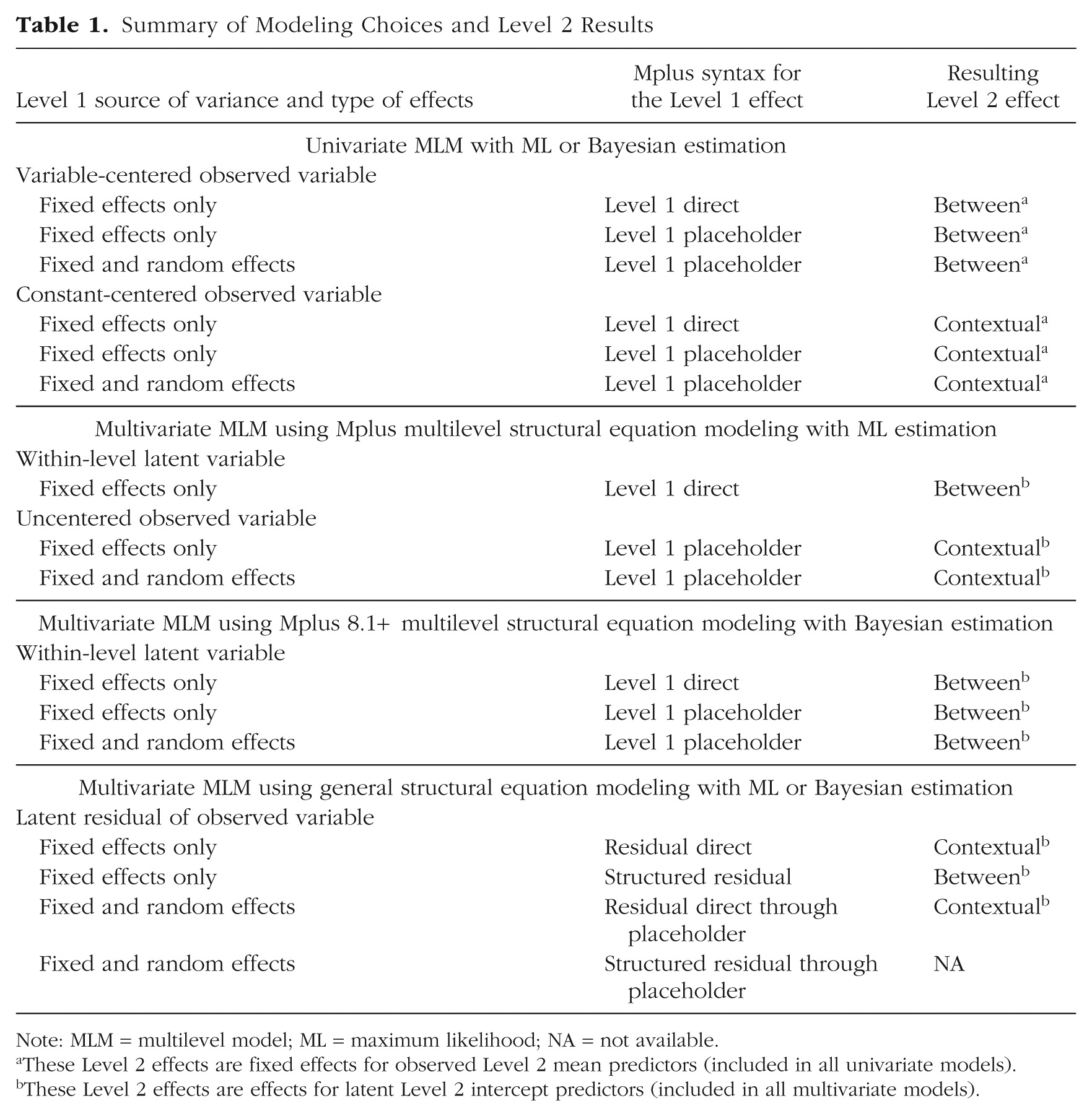
Note: MLM = multilevel model; ML = maximum likelihood; NA = not available.

a

These Level 2 effects are fixed effects for observed Level 2 mean predictors (included in all univariate models).

b

These Level 2 effects are effects for latent Level 2 intercept predictors (included in all multivariate models).

Disclosures

The Supplemental Material for this article (http://journals.sagepub.com/doi/suppl/10.1177/2515245919842770; also available at https://osf.io/mk73j/) includes three types of Mplus files. First, I have included all data, input, and output from the reported simulation. Second, I have included input and output for one replication using the univariate MLMs presented next. Third, I have included input and output for the same replication using the multivariate MLMs, including both multilevel SEM and single-level SEM variants, presented subsequently. For each model, separate files are provided for Bayesian and ML estimation. All materials were initially created in Mplus 8.1 but were subsequently verified to be identical in Mplus 8.2, as expected.

Univariate Multilevel Models

Variance partitioning

Univariate multilevel analyses typically begin with an empty-means (i.e., unconditional-means) model, whose purpose is to quantify how much outcome variance is attributable to each dimension (level) of sampling before predictors are included, as shown in Equation 1:

$$\begin{array}{l}\mathrm{Level}1:y_{wb}={\mathrm{\beta }}_{0b}+e_{wb}\\ \mathrm{Level}2:{\mathrm{\beta }}_{0b}={\mathrm{\gamma }}_{00}+U_{0b}\end{array}$$

(1)

In this equation, y_wb is the outcome for Level 1 within unit w and Level 2 between unit b. At Level 1, the term β_0b is the intercept for Level 2 unit b; β_0b is created by two terms in its Level 2 model. First is the fixed intercept, γ₀₀, which is the grand mean of the Level 2 unit means. Second is U_0b, which is a random intercept that captures the deviation of the mean for Level 2 unit b from the grand mean. The model summarizes the variability across Level 2 units in their U_0b values as Level 2 random intercept variance, denoted as ${\mathrm{\tau }}_{U0}^2$ , which captures variability between Level 2 units due to mean differences. At Level 1, e_wb is a residual for the remaining deviation of the observed y_wb from the model-predicted y_wb. Finally, the model summarizes the variability of the e_wb values across the entire sample as the Level 1 residual variance, denoted as ${\sigma }_e^2$ , which captures the remaining variability within Level 2 units.

These two variance estimates are often used to calculate a useful descriptive statistic, the intraclass correlation, or ICC, which is calculated as follows: ICC = ${\mathrm{\tau }}_{U0}^2$ /( ${\mathrm{\tau }}_{U0}^2$ + ${\sigma }_e^2$ ). The ICC is the proportion of total variance due to intercept (mean) differences between Level 2 units; thus 1 – ICC is the proportion of variance within Level 2 units. For instance, in longitudinal data, the ICC quantifies the variance due to mean differences between persons (at Level 2) relative to the time-specific variance within persons (at Level 1). Likewise, in clustered data, the ICC quantifies the variance due to mean differences between groups (at Level 2) relative to the person-specific variance within groups (at Level 1).

Fixed effects of predictors (i.e., fixed slopes) are then added to the model to explain the outcome variance at their corresponding level of measurement. The term fixed indicates that the slope coefficient will be held constant across Level 2 units (as opposed to random, which indicates that the slope coefficient will be allowed to vary across Level 2 units instead). In two-level models, Level 2 predictors can have only fixed effects. Further, because they have only one source of variance (between Level 2 units), their main effects or interactions can be included directly via their observed variables. To create a meaningful reference point for the intercept and for any simple main effects of interacting predictors, it is customary to center Level 2 predictors, that is, to rescale them so that zero is a meaningful value. Notably, when centering is accomplished by adding or subtracting the same constant in all cases, the fit and predictions of the model will not vary with the centering constant used. Thus, there is no centering constant that would be the wrong choice; different choices will just result in model fixed effects that are more or less useful for directly answering the researchers’ questions.

This is not the case for Level 1 predictors, whose centering can be tricky. This is because Level 1 predictors usually contain both Level 1 and Level 2 sources of variation, just as Level 1 outcomes do (and the extent of each source of Level 1 predictor variance can be quantified by an ICC from an empty-means model, just as the extent of each source of Level 1 outcome variance can be). But when one uses univariate MLM software—and thus the model estimates variance components only for Level 1 outcomes—an analogous variance partitioning for Level 1 predictors requires creating new observed predictor variables through different kinds of centering. As a result, the topic of how to properly specify and interpret the effects of Level 1 observed predictors has received much (needed) attention. The two main options for centering Level 1 predictors are usually referred to as grand-mean centering and group-mean (or person-mean) centering. But given that the centering point is a constant in the former, whereas it is a Level 2 variable in the latter, these options can be thought of more generally as constant centering and variable centering, respectively. Because the results obtained using variable centering in univariate MLMs readily map onto the multivariate MLMs I describe later, I discuss the variable-centering approach for Level 1 predictors first.

Variable centering of Level 1 predictors

Equation 2 provides an example in which variable centering is used to create two new predictors with which to specify the overall main effect of a Level 1 variable, x_wb:

$$\begin{array}{l}\mathrm{Level}1:y_{wb}={\mathrm{\beta }}_{0b}+{\mathrm{\beta }}_{1b}(x_{wb}-{\overline{x}}_b)+e_{wb}\\ \mathrm{Level}2:{\mathrm{\beta }}_{0b}={\mathrm{\gamma }}_{00}+{\mathrm{\gamma }}_{01}({\overline{x}}_b-{\mathrm{C}}_2)+U_{0b}\\ {\mathrm{\beta }}_{1b}={\mathrm{\gamma }}_{10}+U_{1b}\end{array}$$

(2)

Two fixed slopes, γ₀₁ and γ₁₀, and a random slope, U_1b, have been added to Equation 1. First, a new variable, $\overline{x}$ _b , has been created to capture mean differences across Level 2 units; this variable is then centered at the constant C₂ to create a meaningful zero. The fixed slope γ₀₁ of this new Level 2 mean predictor, ( $\overline{x}$ _b – C₂), carries the Level 2 between effect: the impact of having more of x_wb on average than other Level 2 units. For instance, in longitudinal data, the between effect will be due to having more of $\overline{x}$ _b than other people; in clustered data, the between effect will be due to having more of $\overline{x}$ _b than other groups.

Next, the slope β_1b (for Level 2 unit b) in the Level 1 model is defined in its Level 2 model by a fixed slope, γ₁₀, and a random slope, U_1b. It is important to note that β_1b multiplies a new Level 1 observed predictor, which was created by variable-centering the original Level 1 variable at the Level 2 mean, $\overline{x}$ _b . Thus, in the new Level 1 predictor, (x_wb − $\overline{x}$ _b ), a zero value refers to Level 1 units that are at the mean of their Level 2 unit. This variable-centering process removes all mean differences between Level 2 units and leaves only the Level 1 variability within Level 2 units. Consequently, the fixed slope γ₁₀ for the variable-centered predictor (x_wb − $\overline{x}$ _b ) carries the Level 1 within effect: It reflects the impact of having more of x_wb than other Level 1 units within the same Level 2 unit. For example, in longitudinal data, the within effect will be due to a time-varying predictor at a given occasion being greater than the individual’s own mean over time; in clustered data, the within effect will be due to having more of a person-level predictor than others in the group do. In addition, the Level 1 within effect of (x_wb − $\overline{x}$ _b ) is allowed to vary across Level 2 units via U_1b, a random slope that captures the deviation of the Level 1 within slope for Level 2 unit b from the grand-mean within slope across Level 2 units (the fixed Level 1 within slope γ₁₀). This means that each Level 2 unit gets its own Level 1 within slope for (x_wb − $\overline{x}$ _b ). The estimated variance of U_1b, the Level 2 random slope variance, denoted as ${\mathrm{\tau }}_{U1}^2$ , describes the amount of variability between Level 2 units in the Level 1 within slope for (x_wb − $\overline{x}$ _b ).

This model specification (variable-centered Level 1 predictors; see Table 1) can be used in any univariate MLM software (and also applies to multilevel SEMs in Mplus). It is illustrated in Figure 1a. Note that the two observed predictors for x_wb in Figure 1a have been created to capture the same types of level-specific variability that were created by the model for the y_wb outcome. That is, the Level 2 mean predictor ( $\overline{x}$ _b – C₂) is intended to mimic the Level 2 outcome random intercept U_0b, and the Level 1 deviation predictor (x_wb − $\overline{x}$ _b ) is intended to mimic the Level 1 outcome residual e_wb. Because these new predictors contain only level-specific variability (and are thus uncorrelated), each of their fixed effects has a single possible interpretation and purpose: The between effect γ₀₁ of the Level 2 mean predictor ( $\overline{x}$ _b – C₂) will reduce the Level 2 random intercept variance ( ${\mathrm{\tau }}_{U0}^2$ ), and the within effect γ₁₀ of the Level 1 deviation predictor (x_wb − $\overline{x}$ _b ) will reduce the Level 1 residual variance ( ${\sigma }_e^2$ ). The model also includes a covariance between the Level 2 random intercept and slope, ( ${\mathrm{\tau }}_{U01}$ ), although this is not explicitly included in Equation 2.

Fig. 1.

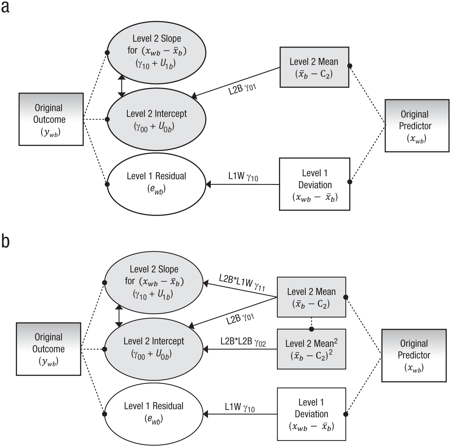
Depiction of univariate multilevel models with a variable-centered Level 1 predictor: (a) the model in Equation 2 and (b) the model in Equation 3. Rectangles indicate observed variables, ovals indicate estimated variables, single-headed arrows indicate fixed effects, two-headed arrows indicate covariances, and dotted lines link model variables to their original sources. Gray fill is used for Level 2 terms, and white fill is used for Level 1 terms (and thus a gradient of gray and white is used for the original predictor and outcome variables). L1W = Level 1 within effect; L2B = Level 2 between effect.

Figure 1a suggests another role that the Level 2 mean predictor ( $\overline{x}$ _b – C₂) could play: Just as it explains the Level 2 random intercept variance ( ${\mathrm{\tau }}_{U0}^2$ ), it might also explain the Level 2 random slope variance ( ${\mathrm{\tau }}_{U1}^2$ ) in the Level 1 within effect, as shown in Equation 3:

$$\begin{array}{l}\mathrm{Level}1:y_{wb}={\mathrm{\beta }}_{0b}+{\mathrm{\beta }}_{1b}(x_{wb}-{\overline{x}}_b)+e_{wb}\\ \mathrm{Level}2:{\mathrm{\beta }}_{0b}={\mathrm{\gamma }}_{00}+{\mathrm{\gamma }}_{01}({\overline{x}}_b-{\mathrm{C}}_2)+\\ \underset{\_}{{\mathrm{\gamma }}_{02}({\overline{x}}_b-{\mathrm{C}}_2\mathrm{)}({\overline{x}}_b-{\mathrm{C}}_2)}+U_{0b}\\ {\mathrm{\beta }}_{1b}={\mathrm{\gamma }}_{10}+\underset{\_}{{\mathrm{\gamma }}_{11}({\overline{x}}_b-{\mathrm{C}}_2)}+U_{1b}\end{array}$$

(3)

Two new fixed effects (underlined for emphasis) have been added. One is γ₁₁, the fixed slope for the Level 2 mean predictor ( $\overline{x}$ _b – C₂), which has been added to the Level 2 model for β_1b. This creates a cross-level interaction between the Level 2 and Level 1 predictors: γ₁₁ is the moderation of the Level 1 within effect by the Level 2 mean predictor. For instance, in longitudinal data, the within effect of having more x_wb than usual (x_wb − $\overline{x}$ _b ) may depend on how much x_wb a person has on average ( $\overline{x}$ _b – C₂); in clustered data, the within effect of having more x_wb than other people in the group (x_wb − $\overline{x}$ _b ) may depend on how much x_wb the group has on average ( $\overline{x}$ _b – C₂).

The other new term—γ₀₂, the fixed effect of ( $\overline{x}$ _b – C₂)( $\overline{x}$ _b – C₂) predicting the Level 2 intercept—may seem odd at first glance, but it serves to keep the model moderation symmetric across levels (see Hoffman, 2015, for an elaboration of the present case, or Hofmann & Gavin, 1998, for a parallel example of dual-level moderation by a pure Level 2 predictor). This is because any Level 2 predictor could moderate both the Level 1 within and the Level 2 between effects of x_wb. In the present case, if the Level 2 mean predictor ( $\overline{x}$ _b – C₂) moderates the Level 1 within effect (through the cross-level interaction γ₁₁), then it could also moderate the Level 2 between effect. Equation 3 captures the latter effect by adding the Level 2 interaction γ₀₂ for the squared effect of ( $\overline{x}$ _b – C₂). The model from Equation 3 is depicted in Figure 1b, in which γ₀₂, the effect of the squared Level 2 ( $\overline{x}$ _b – C₂), reduces the Level 2 random intercept variance ( ${\mathrm{\tau }}_{U0}^2$ ), and γ₁₁, the cross-level interaction of (x_wb − $\overline{x}$ _b ) and ( $\overline{x}$ _b – C₂), reduces the Level 2 random slope variance ( ${\mathrm{\tau }}_{U1}^2$ ).

The use of variable centering (as just demonstrated) arguably provides for the most direct interpretation of the model effects: Because the Level 1 predictor has been partitioned a priori into two level-specific observed predictor variables, each clearly pertains to a Level 2 between effect or a Level 1 within effect. And as in other linear models, omitting any fixed main effects or interaction effects of these level-specific predictors implies that the missing effects would be zero. This is not the case when Level 1 predictors are centered using a constant instead, as I describe next.

Constant centering of Level 1 predictors

Rather than center the Level 1 predictor using the Level 2 mean $\overline{x}$ _b , one might instead choose to center it at a constant: x_wb – C₁. With this choice, it may be less obvious why the Level 2 mean predictor ( $\overline{x}$ _b – C₂) from the previous models is still necessary. To understand why it is indeed still needed, consider the impact of its omission, as in Equation 4:

$$\begin{array}{l}\mathrm{Level}1:y_{wb}={\mathrm{\beta }}_{0b}+{\mathrm{\beta }}_{1b}(x_{wb}-{\mathrm{C}}_1)+e_{wb}\\ \mathrm{Level}2:{\mathrm{\beta }}_{0b}={\mathrm{\gamma }}_{00}+U_{0b}\\ {\mathrm{\beta }}_{1b}={\mathrm{\gamma }}_{10}+U_{1b}\end{array}$$

(4)

In this equation, one fixed effect, instead of two, is used to capture the overall effect of the Level 1 predictor. Although the use of the centering constant C₁ does create a meaningful intercept, it does not solve a bigger, more critical problem: To the extent that the Level 1 predictor x_wb varies over both Level 1 and Level 2 units, it needs to be represented by two distinct model predictors, not one (just as the presence of two sources of variability in the y_wb outcome signals the need for a multilevel model in the first place). Otherwise, both sources of predictor variability—Level 1 within and Level 2 between—are constrained to have the same fixed effect. This single effect is given in Equation 4 by γ_10, a likely useless estimate known more formally as a conflated effect (Preacher, Zhang, & Zyphur, 2011), or less formally as a smushed effect (Hoffman, 2015).

Whether one fixed effect can do the work of two fixed effects is an empirical question, answerable by including the main effect of the Level 2 mean predictor, as in Equation 5:

$$\begin{array}{l}\mathrm{Level}1:y_{wb}={\mathrm{\beta }}_{0b}+{\mathrm{\beta }}_{1b}(x_{wb}-{\mathrm{C}}_1)+e_{wb}\\ \mathrm{Level}2:{\mathrm{\beta }}_{0b}={\mathrm{\gamma }}_{00}+{\mathrm{\gamma }}_{01}({\overline{x}}_b-{\mathrm{C}}_2)+U_{0b}\\ {\mathrm{\beta }}_{1b}={\mathrm{\gamma }}_{10}+U_{1b}\end{array}$$

(5)

The Level 2 mean predictor (x– $\overline{x}$ _b − C₂) now has a separate fixed main effect of γ₀₁. This model specification (a constant-centered Level 1 predictor in a univariate MLM; see Table 1) is depicted in Figure 2a, which shows how the two fixed effects work together to create a different effect at Level 2 than at Level 1. As background for how this happens, consider how a bivariate correlation differs from a regression slope in a multiple-predictor regression model: The correlation reflects an unconditional association, whereas the regression slope reflects each predictor’s unique effect, controlling for the other predictors in the model. Here, the Level 1 predictor (x_wb – C₁) still contains both Level 1 and Level 2 variability, whereas the Level 2 mean predictor ( $\overline{x}$ _b − C₂) contains only Level 2 variability. Consequently, the unique fixed effect of the Level 1 predictor (given by γ₁₀) is now the Level 1 within effect, just as it should be.

Fig. 2.

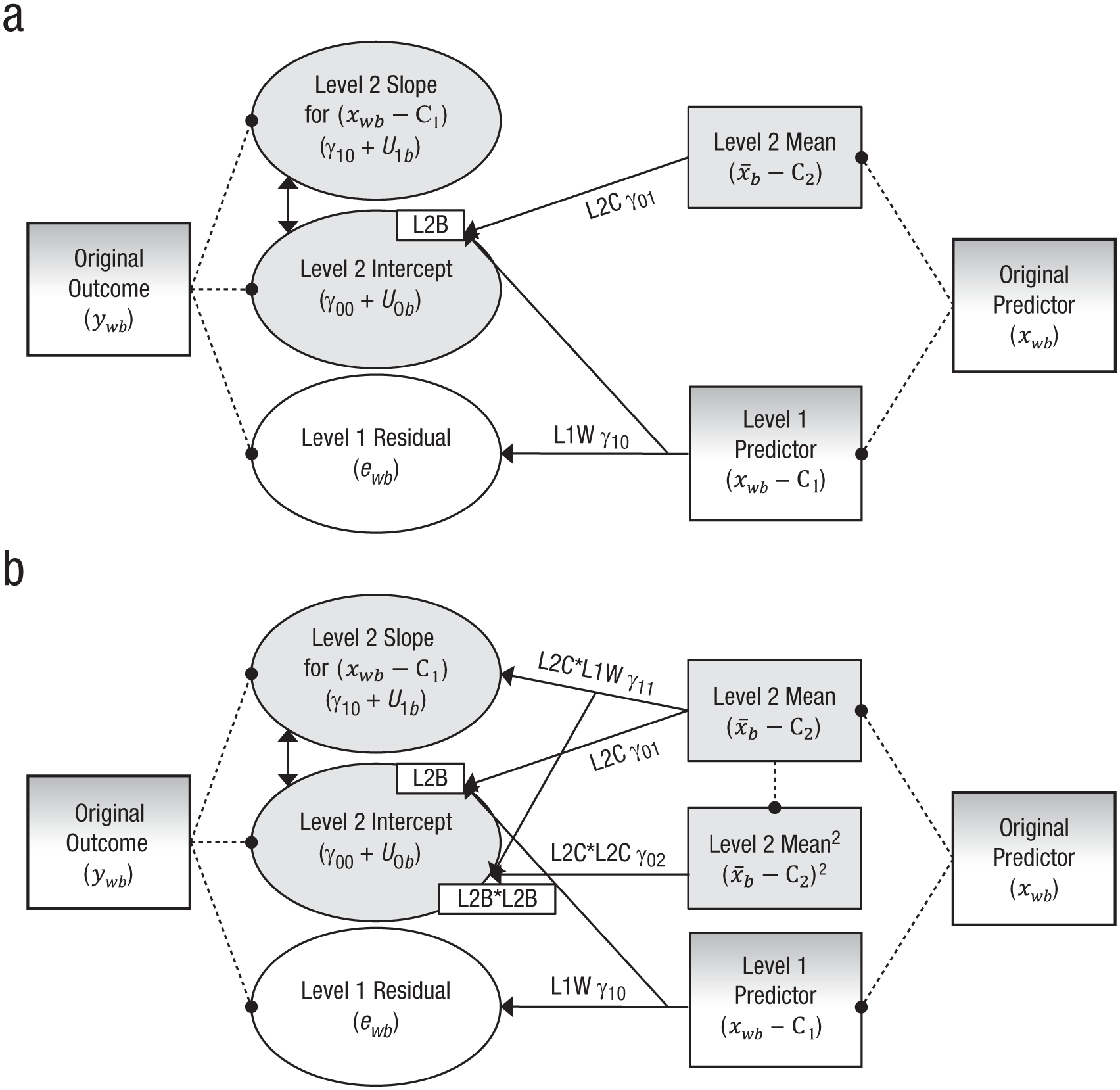
Depiction of univariate multilevel models with a constant-centered Level 1 predictor: (a) the model in Equation 5 and (b) the model in Equation 7. Rectangles indicate observed variables, ovals indicate estimated variables, two-headed arrows indicate covariances, and dotted lines link model variables to their original sources. Single-headed arrows indicate fixed effects; arrows originating from another arrow indicate that the Level 1 fixed effect is needed to get to the full between-level effect indicated by the box labeled “L2B” or “L2B*L2B” at the “Level 2 Intercept” oval. Gray fill is used for Level 2 terms, and white fill is used for Level 1 terms (and thus a gradient of gray and white is used for the original predictor and outcome variables, as well as the Level 1 predictor). L2C = Level 2 contextual effect; L1W = Level 1 within effect; L2B = Level 2 between effect.

Correctly interpreting the fixed effect of the Level 2 mean predictor in this model can be tricky. Because some of the outcome’s Level 2 random intercept variance has already been explained by the Level 2 variability still contained in the constant-centered Level 1 predictor, the unique fixed effect of the Level 2 mean predictor becomes the Level 2 contextual effect, which can be understood from two complementary perspectives. First, from a statistical point of view, the Level 2 contextual effect is how the Level 2 between effect differs from the Level 1 within effect: contextual effect = between effect – within effect. Thus, whether a single fixed effect for a Level 1 predictor is sufficient is tested formally as the significance of the Level 2 contextual effect. Second, from a conceptual point of view, the Level 2 contextual effect is the incremental effect of the Level 2 mean predictor after controlling for the original Level 1 predictor. If a given Level 1 unit has a high x_wb value, one might infer that its Level 2 unit also has a high mean ( $\overline{x}$ _b ). The Level 2 contextual effect captures the additional effect of the Level 2 unit not inferable from the current Level 1 unit. A little later, I provide examples of when a Level 2 contextual effect might be more useful than a Level 2 between effect and vice versa.

Although the need for multilevel models to include contextual main effects is frequently recognized, the role of contextual effects in interactions has received less attention. Consider what happens when a cross-level interaction is added to the previous model, as in Equation 6:

$$\begin{array}{l}\mathrm{Level}1:y_{wb}={\mathrm{\beta }}_{0b}+{\mathrm{\beta }}_{1b}(x_{wb}-{\mathrm{C}}_1)+e_{wb}\\ \mathrm{Level}2:{\mathrm{\beta }}_{0b}={\mathrm{\gamma }}_{00}+{\mathrm{\gamma }}_{01}({\overline{x}}_b-{\mathrm{C}}_2)+U_{0b}\\ {\mathrm{\beta }}_{1b}={\mathrm{\gamma }}_{10}+{\mathrm{\gamma }}_{11}({\overline{x}}_b-{\mathrm{C}}_2)+U_{1b}\end{array}$$

(6)

As before, γ₁₁ is the fixed slope for the cross-level interaction between the Level 1 predictor (x_wb – C₁) and the Level 2 mean predictor ( $\overline{x}$ _b − C₂). But because the Level 1 predictor still contains both Level 1 and Level 2 variability, the moderation by the Level 2 mean predictor ( $\overline{x}$ _b – C₂) is forced to be the same at within Level 1 and between Level 2. That is, γ₁₁ is actually a conflated, or smushed, interaction (for elaboration, see Hoffman, 2015; Hofmann & Gavin, 1998; or Preacher, Zhang, & Zyphur, 2016).

This problem can be solved analogously to the way it was solved for the main effect of Level 1 x_wb: by adding a second interaction term that allows separate moderation by ( $\overline{x}$ _b – C₂) at each level, as shown in Figure 2b and in Equation 7:

$$\begin{array}{l}\mathrm{Level}1:y_{wb}={\mathrm{\beta }}_{0b}+{\mathrm{\beta }}_{1b}(x_{wb}-{\mathrm{C}}_1)+e_{wb}\\ \mathrm{Level}2:{\mathrm{\beta }}_{0b}={\mathrm{\gamma }}_{00}+{\mathrm{\gamma }}_{01}({\overline{x}}_b-{\mathrm{C}}_2)+\\ {\mathrm{\gamma }}_{02}({\overline{x}}_b-{\mathrm{C}}_2)({\overline{x}}_b-{\mathrm{C}}_2)+U_{0b}\\ {\mathrm{\beta }}_{1b}={\mathrm{\gamma }}_{10}+{\mathrm{\gamma }}_{11}({\overline{x}}_b-{\mathrm{C}}_2)+U_{1b}\end{array}$$

(7)

In this model, γ₀₂, the new fixed effect for ( $\overline{x}$ _b – C₂)( $\overline{x}$ _b – C₂), allows for a difference in moderation across levels. As a result, γ₁₁ is now a unique effect for how the Level 1 within effect of x_wb is moderated by ( $\overline{x}$ _b – C₂), and the new fixed effect γ₀₂ is a Level 2 contextual interaction. It can be understood statistically as how the within-level moderation by the Level 2 mean predictor ( $\overline{x}$ _b – C₂) differs from the between-level moderation by the Level 2 mean predictor ( $\overline{x}$ _b – C₂), or conceptually as the Level 2 incremental moderation by the Level 2 mean predictor ( $\overline{x}$ _b – C₂) after controlling for within-level moderation by the Level 2 mean predictor ( $\overline{x}$ _b – C₂).

Regardless of the ease of their interpretation or theoretical interest, contextual effects are very likely to be present in multilevel data and cannot be ignored, no matter what one’s research hypotheses or interests might be. This is because, in addition to theoretical reasons for distinct types of variation at each level of sampling, contextual effects are expected simply because fixed effects are unstandardized coefficients: Their values depend on the level-specific standard deviations of the predictor and outcome. So even if all variables are standardized to the same scale, their fixed effects will differ across levels whenever the predictors and outcomes have different ICCs (and thus different absolute amounts of variance they can share at each level).

Given that Level 1 samples are larger than Level 2 samples (and often much larger), Level 1 within effects will be estimated with more precision than Level 2 between effects. Consequently, conflated (or smushed) effects will more strongly resemble Level 1 within effects than Level 2 between effects, which causes a misspecified Level 2 model in which contextual effects are falsely assumed to be zero (Raudenbush & Bryk, 2002). Further, even if a Level 2 contextual effect were initially nonsignificant, this might not be the case after the addition of other predictors, as the unique contributions of a predictor may differ across levels (and thus require a contextual effect in subsequent models). Thus, the safest course of action is to always address the possibility of distinct fixed effects at every level at which a predictor has variability: at Level 2 only for Level 2 predictors, but at both levels for Level 1 predictors.

Equivalence across methods of centering

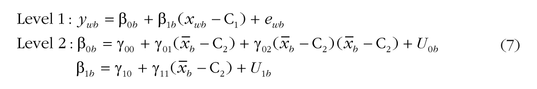
As first derived for main effects by Kreft, de Leeuw, and Aiken (1995), the mapping of the fixed effects of the variable-centered (VC) model in Equation 3 to those of the constant-centered (CC) model in Equation 7 is given in Table 2 (which extends the derivation beyond main effects to include cross-level interactions). In general, once a parallel effect of the Level 2 mean predictor ( $\overline{x}$ _b – C₂) has been included for every Level 1 main effect or interaction, the Level 1 fixed effects become within effects as desired in both models, even though they apply to different Level 1 predictor variables: (x_wb − $\overline{x}$ _b ) in the VC Level 1 model and (x_wb – C₁) in the CC Level 1 model. Meanwhile, even though the same Level 2 mean predictor variable ( $\overline{x}$ _b – C₂) is used in both models, its Level 2 fixed effects switch from between (total Level 2) effects in the VC model to contextual (incremental Level 2) effects in the CC model. That is, the effect of the exact same Level 2 predictor is interpreted differently depending on which type of the Level 1 predictor it is paired with—tricky!

Table 2.

Relationship Between Model Fixed Effects Obtained With the Two Level 1 Centering Methods

Fixed effect	Variable-centered Level 1 model in Equation 3	Constant-centered Level 1 model in Equation 7
Intercept	γ00	γ00
Level 1 within main effect	γ10	γ10
Level 2 contextual main effect	γ01 – γ10	γ01
Level 2 between main effect	γ01	γ01 + γ10
Level 1 Within Effect × Level 2 Between Effect or Level 1 Within Effect × Level 2 Contextual Effect	γ11	γ11
Level 2 Contextual Effect × Level 2 Contextual Effect	γ02 – γ11	γ02
Level 2 Between Effect × Level 2 Between Effect	γ02	γ02 + γ11

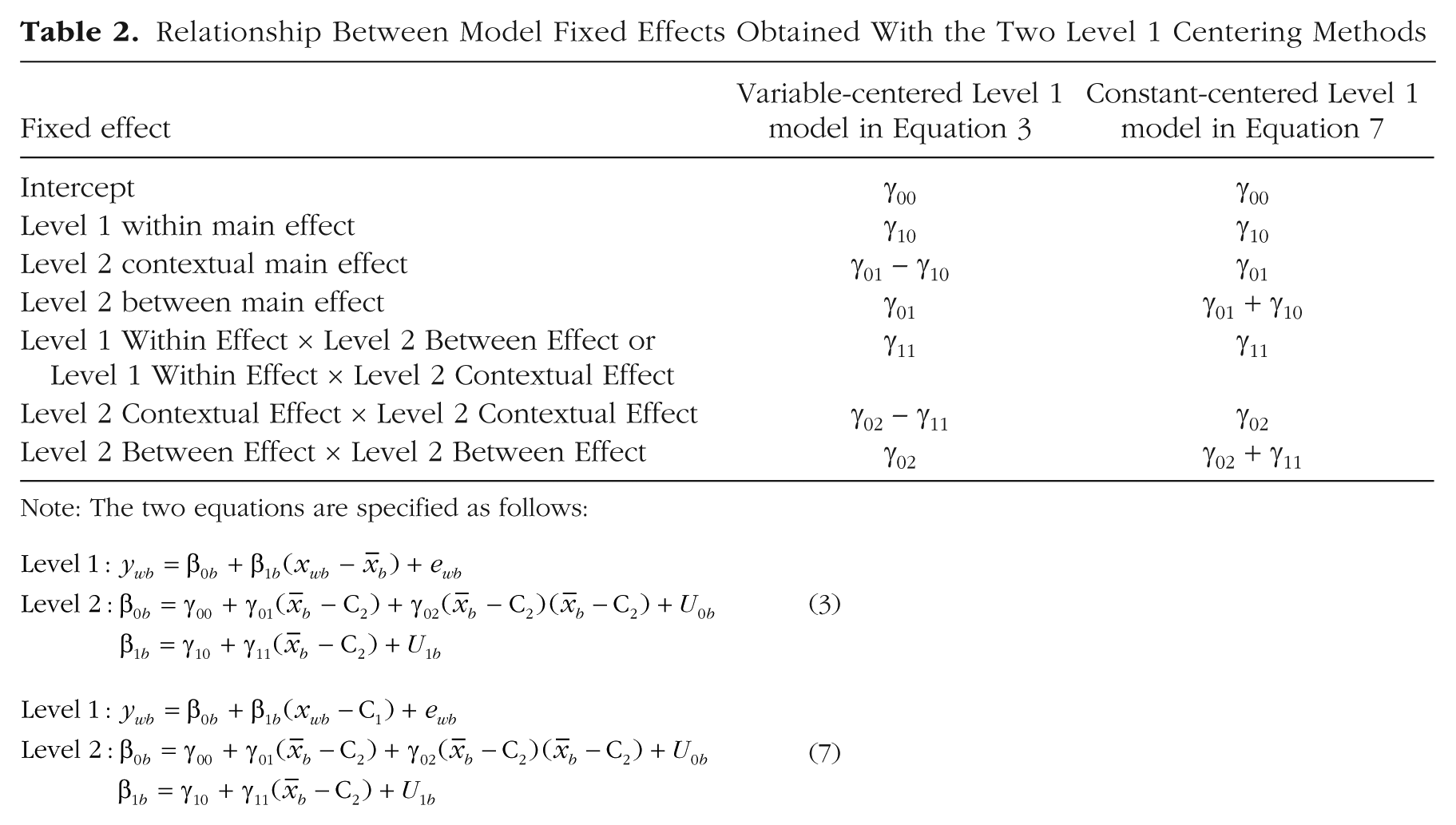
Note: The two equations are specified as follows:

$\begin{array}{l}\mathrm{Level}1:y_{wb}={\mathrm{\beta }}_{0b}+{\mathrm{\beta }}_{1b}(x_{wb}-{\overline{x}}_b)+e_{wb}\\ \mathrm{Level}2:{\mathrm{\beta }}_{0b}={\mathrm{\gamma }}_{00}+{\mathrm{\gamma }}_{01}({\overline{x}}_b-{\mathrm{C}}_2)+{\mathrm{\gamma }}_{02}({\overline{x}}_b-{\mathrm{C}}_2)({\overline{x}}_b-{\mathrm{C}}_2)+U_{0b}\\ {\mathrm{\beta }}_{1b}={\mathrm{\gamma }}_{10}+{\mathrm{\gamma }}_{11}({\overline{x}}_b-{\mathrm{C}}_2)+U_{1b}\end{array}$    (3)

$\begin{array}{l}\mathrm{Level}1:y_{wb}={\mathrm{\beta }}_{0b}+{\mathrm{\beta }}_{1b}(x_{wb}-{\mathrm{C}}_1)+e_{wb}\\ \mathrm{Level}2:{\mathrm{\beta }}_{0b}={\mathrm{\gamma }}_{00}+{\mathrm{\gamma }}_{01}({\overline{x}}_b-{\mathrm{C}}_2)+{\mathrm{\gamma }}_{02}({\overline{x}}_b-{\mathrm{C}}_2)({\overline{x}}_b-{\mathrm{C}}_2)+U_{0b}\\ {\mathrm{\beta }}_{1b}={\mathrm{\gamma }}_{10}+{\mathrm{\gamma }}_{11}({\overline{x}}_b-{\mathrm{C}}_2)+U_{1b}\end{array}$    (7)

So when is each type of Level 2 effect—between or contextual—likely to be more useful? Level 2 contextual effects are often of interest in clustered designs, in which they provide the unique effect of Level 2 group characteristics above and beyond Level 1 person characteristics (see Hofmann & Gavin, 1998). For this case, constant centering Level 1 predictors will ensure that all corresponding Level 2 effects directly represent the contextual effects of interest. For example, consider free-lunch status (0 = no, 1 = yes) as a predictor of the achievement of Level 1 students nested in Level 2 schools. A binary Level 1 predictor representing students’ free-lunch status can be included directly in the model (which would be akin to constant centering this predictor at 0). But to the extent that schools differ in their free-lunch rates, and these school-level differences in turn matter for schools’ mean achievement, the Level 1 effect of students’ free-lunch status will be the smushed (and therefore meaningless) effect without a corresponding school-level free-lunch predictor: the percentage of students who receive free lunch at each school (i.e., the mean across students in the sample or the percentage for each school as obtained from better sources). Once both predictors have been included, as in the main-effects model in Equation 5, the student-level predictor carries the Level 1 within effect: γ₁₀ is the gap in achievement between students at the same school who do and do not get free lunch. The school-level free-lunch predictor carries the Level 2 contextual effect: γ₀₁ is the incremental difference in school-level achievement per unit difference in this predictor (i.e., going from 0% to 100% free-lunch rate) after controlling for student-level free-lunch status; it conveys the extent to which schools with higher rates of poverty might see lower achievement in all of their students, even those who do not get free lunch. The Level 2 between effect would be given by γ₁₀ + γ₀₁, which would instead convey the total school-level free-lunch effect not controlling for students’ free-lunch status.

In contrast, contextual effects may be less useful in longitudinal designs, in which the Level 1 occasions are not unique entities (the way that Level 1 students are). For this case, it can be more helpful to variable-center Level 1 predictors so that all Level 2 effects will directly represent between effects (Hoffman & Stawski, 2009). For example, consider stress and health measured at multiple Level 1 occasions nested in Level 2 persons. In a main-effects model as in Equation 2, the variable-centered Level 1 predictor (x_wb − $\overline{x}$ _b ) carries the Level 1 within effect: γ₁₀ is the change in health at a given occasion associated with a 1-unit change in stress within the same person at that occasion. The Level 2 predictor (created from the person’s mean stress across occasions, $\overline{x}$ _b ) carries the Level 2 between effect: γ₀₁ is the difference in average health per unit difference in person-level stress, not controlling for stress at that occasion. Said more simply, the Level 1 within effect is the effect of more stress than usual, whereas the Level 2 between effect is the effect of more stress than other people. The Level 2 contextual effect, γ₀₁ – γ₁₀, instead conveys the incremental effect of the person’s mean stress after controlling for stress at that occasion.

Although Table 2 indicates how to find the model-implied Level 2 effects not directly provided by the estimated fixed effects, these conversions will hold exactly only if the Level 1 effect does not have a random slope (see Kreft et al., 1995, for a derivation). Otherwise, they will only be approximate, as in the case of the example models here that have included a random slope for the Level 1 predictor. This is because the random slope will apply to a different Level 1 predictor depending on the model: to (x_wb − $\overline{x}$ _b ) in the VC Level 1 model and to (x_wb – C₁) in the CC Level 1 model. So, given that the variance in the Level 2 mean $\overline{x}$ _b has been removed from the predictor in the VC Level 1 model, the estimated Level 2 random slope variances will differ between the VC and CC models. In addition, given that the model intercept is defined as the expected outcome when all predictors are zero, the variance of the Level 2 random intercept will differ between these models because they differ in when each Level 1 predictor has a zero value: when x_wb equals $\overline{x}$ _b in the VC model, but when x_wb equals C₁ in the CC model.

These differences in the definition of the random intercept variance can result in differences in the covariance between the random intercept and the random slope, as well as differences in the random slope variance, as described by Raudenbush and Bryk (2002). Whereas every Level 2 unit is likely to have Level 1 values at or near the Level 2 mean $\overline{x}$ _b , every Level 2 unit may not have Level 1 values observed near the constant C₁, and this becomes even more likely as the ICC for the Level 1 predictor increases. As a result, the greater the extrapolation required for the predicted random intercepts to get to where x_wb equals C₁ in the CC Level 1 model, the more shrinkage those random intercepts may have: They will be biased toward the fixed intercept. This shrinkage can then propagate to the random slopes, which may then be flattened by the less extreme intercepts. As a result, the random slope variance may be downwardly biased (too small) in the CC Level 1 model relative to the VC Level 1 model. For this reason, Raudenbush and Bryk recommended the VC Level 1 model over the CC Level 1 model for estimating random slopes. As I show later, the same pattern of discrepancy arises in multivariate MLMs with model-estimated predictor variables.

Multivariate Multilevel Models

Although Figures 1 and 2 were designed to illustrate differences between models using different centering methods for Level 1 predictors, they also highlight an odd asymmetry in how variables with level-specific variability are addressed in univariate MLMs. That is, why is it that level-specific latent variables (variance components) for Level 1 outcomes are estimated by the model, but an analogous variance partitioning for Level 1 predictors must instead be accomplished using observed variables? Why not treat Level 1 predictors and Level 1 outcomes similarly instead? This is the rationale for multivariate MLMs, which provide model-based variance partitioning for all Level 1 variables—predictors and outcomes. How univariate and multivariate MLMs differ can be illustrated by visualizing new versions of Figures 1 and 2 in which the rectangles for the observed predictor variables (in univariate MLM) are replaced with ovals for model-estimated latent predictor variables (i.e., Level 2 intercepts and Level 1 residuals in multivariate MLM).

Why use multivariate MLMs instead of univariate MLMs?

Because of the recent availability of software for estimating multivariate MLMs, comparisons between approaches have become increasingly of interest. In their seminal work, Lüdtke et al. (2008) examined differences between univariate and multivariate MLMs (using ML estimation) as a function of sample size and predictor ICC. They found that Level 2 contextual fixed effects were downwardly biased in univariate relative to multivariate MLMs, and to a greater extent with smaller Level 1 samples and smaller predictor ICCs. But they also found greater variability in the multivariate MLM results when less information was available for estimating the Level 2 random intercept variance for the predictor (i.e., when Level 2 samples were smaller and ICCs were lower). Preacher et al. (2011) replicated these findings and extended them to a mediation framework.

In addition to the benefits found in those studies, multivariate MLMs have a critical advantage whenever both a Level 1 predictor and a Level 1 outcome contain Level 2 variability in the random slope of another predictor. Consider a longitudinal example of Level 1 occasions nested in Level 2 persons, in which a time-varying Level 1 predictor and a time-varying Level 1 outcome both contain Level 2 random variability in change over time (i.e., the extent of change over time differs across persons in both Level 1 variables). In this case, univariate MLMs are even less preferred: Whereas an observed Level 2 mean predictor can mimic its model-estimated random intercept variability to some extent, no analogous observed variable can adequately capture the variability in the predictor’s random time slope. So a multivariate MLM is needed to distinguish the effects of two kinds of Level 2 predictor variability: variability in the predictor’s intercept and in its time slope. Otherwise, if the predictor’s Level 2 random time slope cannot be included (as in univariate MLMs), the predictor’s Level 1 within fixed effect will be biased toward the missing Level 2 random slope effect (Hoffman, 2015).

Challenges in specifying and interpreting multivariate MLMs

To summarize, relative to univariate MLMs, multivariate MLMs offer greater flexibility for examining complex relationships across multiple sources of sampling simultaneously, in some instances with less bias, but with greater complexity of estimation. Yet it is important to keep in mind that properly specifying multivariate MLMs still requires careful attention to levels of analysis: It is essential to distinguish Level 2 between effects and Level 1 within effects via Level 2 contextual effects. But which centering method has been used for Level 1 predictors is often far less transparent in multivariate MLMs than in univariate MLMs, and thus it can be unclear exactly which type of Level 2 effect—between or contextual—the multivariate MLM output is providing. As I noted earlier, multivariate MLMs can currently be estimated in two primary frameworks: as multilevel SEMs or as single-level SEMs. Although many different software packages are commonly used for single-level SEMs, multilevel SEMs are most frequently estimated using Mplus. Accordingly, I have based the examples that follow on Mplus, but the multivariate MLM concepts I discuss should readily apply to other software programs.

Mplus (up to Version 8.2 as of this writing) is a flexible and comprehensive program for estimating latent-variable models, including MLMs, SEMs, and their intersections. Mplus first began with ML estimation, and more recently has expanded its offerings to Bayesian estimation as well. Despite this software’s popularity, what is not often recognized is how different variants of its syntax for specifying multivariate MLMs will result in different Level 2 model effects. The consequences of these syntax variants, when each kind of estimation is used, are summarized in Table 1 and elaborated in the next section.

First, let us consider what happens when a Level 1 fixed effect (e.g., slope of Level 1 x predicting Level 1 y) is requested directly in the Level 1 %WITHIN% model (e.g., y ON x;). In this case, the same model specification is used in ML and Bayesian estimation. The Level 1 x predictor is partitioned—via a process Asparouhov and Muthén (2019) called latent centering—into two level-specific unobserved (latent) variables: a Level 2 intercept formed from fixed and random effects, and a Level 1 residual; this is the same process that already occurs for any Level 1 y outcome. So the Level 1 fixed effect refers to the regression of the Level 1 residual for y on the Level 1 residual for x, and this slope must be the Level 1 within effect, because neither Level 1 latent variable contains Level 2 mean variability. That is, the Level 1 fixed effect of a latent-centered Level 1 predictor is the model-based analogue of the Level 1 fixed effect provided by a variable-centered Level 1 observed predictor (x_wb − $\overline{x}$ _b ). As a result, the corresponding Level 2 fixed effect in the %BETWEEN% model (y ON x;)—the regression slope of the Level 2 intercept for y on the Level 2 intercept for x—must be the Level 2 between effect. That is, the Level 2 fixed effect of a latent-centered Level 1 predictor is the model-based analogue of the Level 2 fixed effect obtained from the Level 2 observed mean predictor ( $\overline{x}$ _b ) when paired with a variable-centered Level 1 observed predictor (x_wb − $\overline{x}$ _b ). Fortunately, because a latent-centered Level 1 predictor contains only Level 1 variability, its Level 1 fixed effect is the within effect regardless of whether the corresponding Level 2 between effect has been included.

Less transparent is what happens when a Level 1 fixed effect is instead requested via latent-variable placeholder syntax in the Level 1 %WITHIN% model (e.g., s | y ON x;). When this syntax variant is used, the Level 1 fixed effect appears in the Level 2 model output as the mean or intercept of the s latent variable ([s];); its random-effect variance is the latent variable’s variance or residual variance (s;). Notably, although this latent-variable placeholder syntax is required to estimate random effects or cross-level interactions involving the x predictor, the consequences of using it (which I describe next) are the same even when these additional parameters are not estimated.

Critically, beginning in Mplus 8.1, which model specification is invoked by the latent-variable placeholder syntax depends on the choice of estimator. So the onus is on the user to realize that even if the exact same syntax is used, a difference in which estimator is used will result in a difference in the interpretation of parameters as a result of concomitant differences in model specification. The more straightforward case is when Bayesian estimation is used, as the placeholder syntax in combination with Bayesian estimation invokes latent centering for the Level 1 predictor, as just described for the Level 1 direct syntax (e.g., y ON x;). So even though the Level 1 effect defined by the placeholder syntax is reported in the output for Level 2 instead of Level 1, it is still the Level 1 within effect, regardless of whether a corresponding Level 2 between fixed effect has been estimated.

In contrast, coupling the latent-variable placeholder syntax with ML estimation invokes the hybrid method of model specification: A new Level 2 latent predictor variable is created through model-based variance partitioning, but the original Level 1 predictor is used in estimating its fixed and random effects (Asparouhov & Muthén, 2019). Thus, the hybrid method’s Level 1 fixed effect refers to the regression of the Level 1 residual for y on the Level 1 observed x predictor, which still contains its Level 2 variability. As a result, if the corresponding Level 2 fixed effect is not included in the %BETWEEN% model, the Level 1 fixed effect will not be the within effect. Instead, it will be the useless smushed effect, because the hybrid method provides the same Level 1 fixed effect as a constant-centered Level 1 observed predictor variable.

As we saw before for univariate MLMs, converting the smushed effect into the Level 1 within effect requires estimating the corresponding Level 2 fixed effect in the %BETWEEN% model. Given the hybrid method’s creation of a latent Level 2 x predictor (in parallel with a latent Level 2 y outcome), the Level 2 fixed effect refers to the regression of the Level 2 intercept for y on the Level 2 intercept for x. But given its pairing with an observed Level 1 x predictor, this Level 2 regression will not provide the Level 2 between effect. Instead, it will provide the Level 2 contextual effect: the incremental effect of the Level 2 x variable after controlling for the effect of the observed Level 1 x variable. That is, the Level 2 fixed effect of a latent Level 2 predictor provided by the hybrid method is the model-based analogue of the Level 2 fixed effect created when an observed Level 2 mean predictor $\overline{x}$ _b is paired with a constant-centered Level 1 observed predictor (x_wb).

So of the two possible model specifications—latent centering and the hybrid method—which should be preferred? To “demonstrate the advantages of latent centering,” Asparouhov and Muthén (2019, p. 132) reported a simulation comparing the results of multivariate MLMs using Bayesian estimation (and latent centering) with the results of multivariate MLMs using ML estimation (and the hybrid method). On the basis of the simulation data they reported in their Table 1, they concluded that the “hybrid method does not perform well” but also that “a complex model transformation is needed to obtain the [ML] results in the original latent centered metric” (p. 126). Readers might infer from their presentation that multivariate MLMs estimated using ML are somehow inferior to those obtained using Bayesian estimation because of differences in estimation, when in fact the differences in these results are expected consequences of the different Level 1 predictors used in the two model specifications.

To better illustrate these differences and their consequences for model interpretation, I next describe the results of a brief simulation study designed as a partial replication of the data in Table 1 of Asparouhov and Muthén (2019). Note that in providing these example models, my goal is not to advocate for one method of estimation over another. Instead, given their choice of estimation method, I want to help analysts (a) ensure that they correctly differentiate their effects at multiple levels of analysis and (b) understand the meaning of their resulting multivariate MLM parameters.

Demonstration via Simulation

Method

Following Asparouhov and Muthén (2019), who used large samples to limit the effect of sampling error, for the current simulation I also generated 1,000 Level 2 samples of 15 Level 1 units each (for a total sample size of 15,000 in each of the 100 replications). The simulation was conducted via the Mplus MONTECARLO routine, which takes user input in the form of variable names and their model parameters, and then generates data consistent with the model specified.

The population model was a multivariate MLM specified as a multilevel SEM. The model’s parameter values are shown in the top panel of Table 3. The Level 1 model related x_wb to y_wb using a fixed effect, and so the matrix for their Level 1 residuals (denoted as R) included a separate variance for each variable, with no covariance between them. Instead of using fixed effects, the model specified the Level 2 relationships (among the Level 2 random slope for Level 1 x_wb and the Level 2 random intercepts for Level 1 x_wb and Level 1 y_wb) in the matrix for the Level 2 random-effect variances and covariances (denoted as G). My reason for doing so was to replicate the population model from Asparouhov and Muthén (2019), but it appears that their motivation may in part have been to speed their Bayesian estimation. That is, whereas their population model could be estimated using their more efficient PX1 Gibbs sampler, multivariate MLMs that instead specify the Level 2 relations using fixed effects and covariances in the same model require their more intensive random-walk (RW) Gibbs sampler.

Table 3.

Population and Analysis Models Used in the Simulation

Population model: all Level 2 covariances
Level 1:xwb = ${\mathrm{\beta }}_{0b}^x$ + $e_{wb}^x$ ywb = ${\mathrm{\beta }}_{0b}^y$ + ${\mathrm{\beta }}_{1b}^y(e_{wb}^x)$ + $e_{wb}^y$ Level 2: ${\mathrm{\beta }}_{0b}^x$ = ${\mathrm{\gamma }}_{00}^x$ + $U_{0b}^x$   ${\mathrm{\gamma }}_{00}^x$ = 0 ${\mathrm{\beta }}_{0b}^y$ = ${\mathrm{\gamma }}_{00}^y$ + $U_{0b}^y$   ${\mathrm{\gamma }}_{00}^y$ = 0 ${\mathrm{\beta }}_{1b}^y$ = ${\mathrm{\gamma }}_{10}^y$ + $U_{1b}^y$    ${\mathrm{\gamma }}_{10}^y$ = −1	$\mathbf{R}=\left(\begin{array}{cc}{\sigma }_{ex}^2& {\sigma }_{ex,ey}\\ {\sigma }_{ex,ey}& {\sigma }_{ey}^2\end{array}\right)=\left(\begin{array}{cc}1& 0\\ 0& 1\end{array}\right)$ $\mathbf{G}=\left(\begin{array}{ccc}{\mathrm{\tau }}_{U0x}^2& {\mathrm{\tau }}_{U0x,U0y}& {\mathrm{\tau }}_{U0x,U1y}\\ {\mathrm{\tau }}_{U0x,U0y}& {\mathrm{\tau }}_{U0y}^2& {\mathrm{\tau }}_{U0y,U1y}\\ {\mathrm{\tau }}_{U0x,U1y}& {\mathrm{\tau }}_{U0y,U1y}& {\mathrm{\tau }}_{U1y}^2\end{array}\right)=\left(\begin{array}{ccc}1& 0.5& 0.3\\ 0.5& 1& 0.2\\ 0.3& 0.2& 1\end{array}\right)$
Analysis model: Level 2 main-effect model*
Level 2: ${\mathrm{\beta }}_{0b}^x$ = ${\mathrm{\gamma }}_{00}^x$ + $U_{0b}^x$ ${\mathrm{\beta }}_{0b}^y$ = ${\mathrm{\gamma }}_{00}^y$ + ${\mathrm{\gamma }}_{01}^y({\mathrm{\beta }}_{0b}^x)$ + $U_{0b}^y$ ${\mathrm{\beta }}_{1b}^y$ = ${\mathrm{\gamma }}_{10}^y$ + $U_{1b}^y$		$\mathbf{G}=\left(\begin{array}{ccc}{\mathrm{\tau }}_{U0x}^2& –& {\mathrm{\tau }}_{U0x,U1y}\\ –& {\mathrm{\tau }}_{U0y}^2& {\mathrm{\tau }}_{U0y,U1y}\\ {\mathrm{\tau }}_{U0x,U1y}& {\mathrm{\tau }}_{U0y,U1y}& {\mathrm{\tau }}_{U1y}^2\end{array}\right)$
Analysis model: cross-level interaction model
Level 2: ${\mathrm{\beta }}_{0b}^x$ = ${\mathrm{\gamma }}_{00}^x$ + $U_{0b}^x$ ${\mathrm{\beta }}_{0b}^y$ = ${\mathrm{\gamma }}_{00}^y$ + ${\mathrm{\gamma }}_{01}^y({\mathrm{\beta }}_{0b}^x)$ + $U_{0b}^y$ ${\mathrm{\beta }}_{1b}^y$ = ${\mathrm{\gamma }}_{10}^y$ + ${\mathrm{\gamma }}_{11}^y({\mathrm{\beta }}_{0b}^x)$ γ + $U_{1b}^y$	$\mathbf{G}=\left(\begin{array}{ccc}{\mathrm{\tau }}_{U0x}^2& –& –\\ –& {\mathrm{\tau }}_{U0y}^2& {\mathrm{\tau }}_{U0y,U1y}\\ –& {\mathrm{\tau }}_{U0y,U1y}& {\mathrm{\tau }}_{U1y}^2\end{array}\right)$
Analysis model: Level 2 interaction model*
Level 1:xwb = ${\mathrm{\beta }}_{0b}^x$ + $e_{wb}^x$ xxwb = ${\mathrm{\beta }}_{0b}^{xx}$ + $e_{wb}^{xx}$ ywb = ${\mathrm{\beta }}_{0b}^y$ + ${\mathrm{\beta }}_{1b}^y(e_{wb}^x)$ + $e_{wb}^y$ Level 2: ${\mathrm{\beta }}_{0b}^x$ = ${\mathrm{\gamma }}_{00}^x$ + $U_{0b}^x$ ${\mathrm{\beta }}_{0b}^{xx}$ = ${\mathrm{\gamma }}_{00}^{xx}$ + $U_{0b}^{xx}$ ${\mathrm{\beta }}_{0b}^y$ = ${\mathrm{\gamma }}_{00}^y$ + ${\mathrm{\gamma }}_{01}^y({\mathrm{\beta }}_{0b}^x)$ + ${\mathrm{\gamma }}_{02}^y({\mathrm{\beta }}_{0b}^{xx})$ + $U_{0b}^y$ ${\mathrm{\beta }}_{1b}^y$ = ${\mathrm{\gamma }}_{10}^y$ + ${\mathrm{\gamma }}_{11}^y({\mathrm{\beta }}_{0b}^x)$ + $U_{1b}^y$	$\mathbf{R}=\left(\begin{array}{ccc}{\sigma }_{ex}^2& {\sigma }_{ex,exx}& -\\ {\sigma }_{ex,exx}& {\sigma }_{ex}^2& {\sigma }_{exx,ey}\\ -& {\sigma }_{exx,ey}& {\sigma }_{ey}^2\end{array}\right)$ $\mathbf{G}=\left(\begin{array}{c}{\mathrm{\tau }}_{U0x}^2\\ {\mathrm{\tau }}_{U0x,U0xx}\\ -\\ -\end{array}\begin{array}{c}{\mathrm{\tau }}_{U0x,U0xx}\\ {\mathrm{\tau }}_{U0xx}^2\\ -\\ {\mathrm{\tau }}_{U0xx,U1y}\end{array}\begin{array}{c}-\\ -\\ {\mathrm{\tau }}_{U0y}^2\\ {\mathrm{\tau }}_{U0y,U1y}\end{array}{\begin{array}{c}-\\ {\mathrm{\tau }}_{U0xx,U1y}\\ {\mathrm{\tau }}_{U0y,U1y}\\ {\mathrm{\tau }}_{U1y}^2\end{array}}^{}\right)$

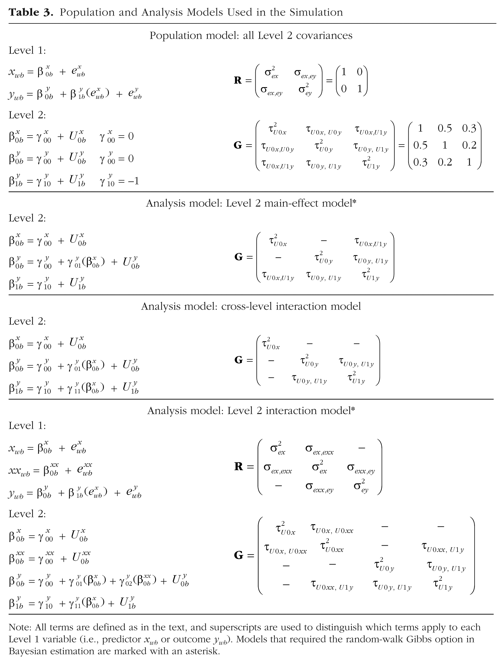
Note: All terms are defined as in the text, and superscripts are used to distinguish which terms apply to each Level 1 variable (i.e., predictor x_wb or outcome y_wb). Models that required the random-walk Gibbs option in Bayesian estimation are marked with an asterisk.

Because the Level 1 effect of x_wb in predicting y_wb in the population model also included a Level 2 random slope, that Level 1 effect had to be specified using latent-variable placeholder syntax in the Level 1 %WITHIN% model (s | y ON x;). The population model that generated the data used Bayesian estimation, and thus the Level 1 predictor was latent centered. Although the population model had the same parameters as used by Asparouhov and Muthén (2019), I changed their parameter values to make my results easier to follow. In my simulations, both Level 1 variables had means of 0, their Level 1 and Level 2 relations were made opposite in sign, and the Level 2 random-effect covariances were varied in size (but all remained positive).

The second through fourth panels of Table 3 provide the three analysis models used. To illustrate changes in parameter interpretation, they mimic the sequence of the univariate MLMs I presented earlier, such that one of the three Level 2 covariances is replaced with a fixed effect in each successive model. Using the population values as start values, I estimated each model twice, once using ML estimation and once using Bayesian estimation, to show how the results from their different model specifications can be made equivalent to the greatest extent possible. For Bayesian estimation, I retained all program defaults for convergence and noninformative prior distributions, such that the only reason for a difference in the results obtained with the two kinds of estimation should be model specification, and not the kind of estimation. The Mplus default PX1 Gibbs sampler could be used only for the cross-level interaction models; the other analysis models required RW Gibbs sampling instead and are marked with an asterisk in Table 3.

Results

Population model

Results from fitting the population model are given in Table 4. As expected, all population values were recovered in the Bayesian solution, which used the same method of latent centering by which the data were generated. In contrast, discrepancies arose for several parameters in the ML solution because this model was not actually equivalent given its use of the hybrid method instead.

Table 4.

Simulation Results for the Population Model

Parameter (Level 2 between model specification)		Level 2 between effect (latent centering with Bayesian estimation)			Level 2 contextual effect (hybrid method with maximum likelihood estimation)
	True value	Mean (estimate)	SD (estimate)	Mean SE	Mean (estimate)	SD (estimate)	Mean SE
Fixed effects
${\mathrm{\gamma }}_{00}^x$    x-intercept	0	0.00	0.03	0.03	0.00	0.03	0.03
${\mathrm{\gamma }}_{00}^y$    y-intercept	0	0.00	0.03	0.03	−0.28	0.06	0.06
${\mathrm{\gamma }}_{10}^y$    Level 1 within effect x → y	−1	−1.00	0.03	0.03	−1.00	0.03	0.03
Variances of Level 2 random effects
${\mathrm{\tau }}_{U0x}^2$    x-intercept	1	1.01	0.05	0.05	1.00	0.05	0.05
${\mathrm{\tau }}_{U0y}^2$   y-intercept	1	1.02	0.05	0.06	3.81	0.22	0.18
${\mathrm{\tau }}_{U1y}^2$   Level 1 within effect x → y	1	1.00	0.05	0.05	0.91	0.05	0.04
Covariances of Level 2 random effects
${\mathrm{\tau }}_{U0x,U0y}$  x-intercept, y-intercept	0.50	0.50	0.04	0.04	1.50	0.08	0.08
${\mathrm{\tau }}_{U0x,U1y}$  x-intercept, Level 1 within effect x → y	0.30	0.31	0.04	0.03	0.28	0.03	0.03
${\mathrm{\tau }}_{U0y,U1y}$  y-intercept, Level 1 within effect x → y	0.20	0.21	0.04	0.04	0.48	0.08	0.07
Correlations of Level 2 random effects
$r_{U0x,U0y}$  x-intercept, y-intercept	0.50	0.49	0.03	0.03	0.77	0.02	0.02
$r_{U0x,U1y}$  x-intercept, Level 1 within effect x → y	0.30	0.30	0.03	0.03	0.29	0.03	0.03
$r_{U0y,U1y}$  y-intercept, Level 1 within effect x → y	0.20	0.21	0.03	0.04	0.25	0.04	0.03
Level 1 residual variances
${\sigma }_{ex}^2$     x	1	1.00	0.01	0.01	1.00	0.01	0.01
${\sigma }_{ey}^2$     y	1	1.00	0.01	0.01	1.01	0.01	0.01

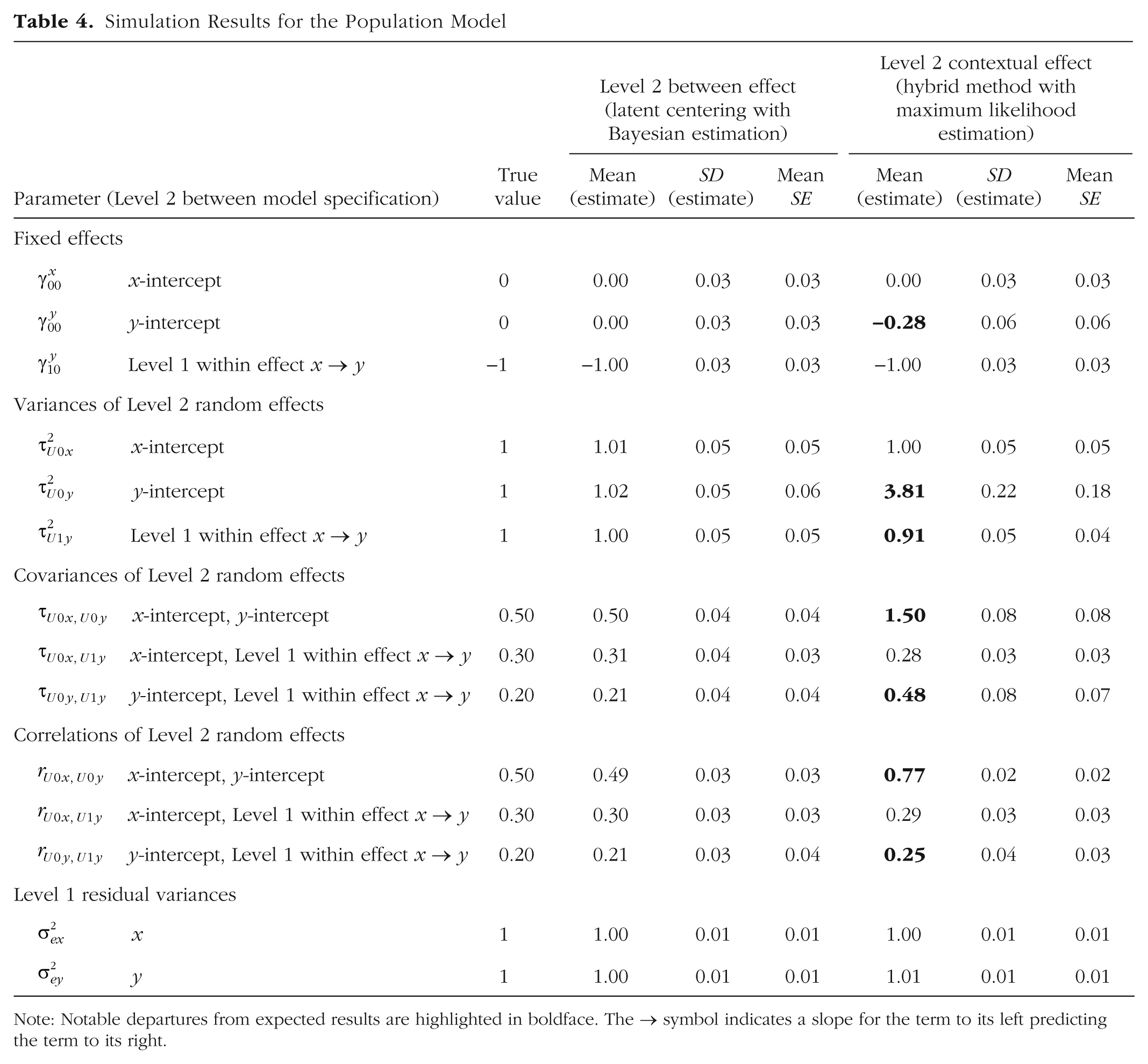
Note: Notable departures from expected results are highlighted in boldface. The → symbol indicates a slope for the term to its left predicting the term to its right.

The first discrepancy is the slight difference in the fixed intercept for y_wb ( ${\mathrm{\gamma }}_{00}^y$ ), which resulted from different definitions of the conditional model intercept. With latent centering and Bayesian estimation, the intercept is specific to when the within part of the Level 1 predictor is 0 (x_wb – ${\mathrm{\beta }}_{0b}^x$ = 0, or $e_{wb}^x$ = 0 in the present case), whereas with the hybrid method and ML estimation, the intercept is specific to when the observed x_wb is 0 (in the present case, when the centering constant C₁ = 0). This difference in ${\mathrm{\gamma }}_{00}^y$ between the Bayesian and ML solutions will recur across models for the same reason: differing Level 1 predictors.

A bigger discrepancy was found in the covariance between the random intercepts for x_wb and y_wb (τ_U0x,U0y), which, as expected, was much more positive with the hybrid method in the ML solution (1.50) than with latent centering in the Bayesian solution (0.50). This discrepancy arose because this intercept covariance provides a different Level 2 relationship in each model: a between relation when latent centering is used (with Bayesian estimation), but a contextual relation when the hybrid method is used (with ML estimation). Given that the Level 1 fixed effect of x_wb in predicting y_wb ( ${\mathrm{\gamma }}_{10}^y$ ) was −1.00, and the Level 2 between intercept covariance was 0.50 (as estimated in the latent-centered Bayesian solution), the covariance of 1.50 (as estimated using the hybrid method with ML) formed the Level 2 contextual effect: the Level 2 between effect minus the Level 1 within effect. However, without a Level 2 fixed effect linking the two Level 2 intercepts, the Level 1 effect obtained using the hybrid method with ML was actually a smushed effect that constrained the Level 1 within and Level 2 between effects to each be −1.00. Because the missing Level 2 between fixed effect should have been 0.50 instead, the y_wb random intercept variance ( ${\mathrm{\tau }}_{U0y}^2$ ) obtained using the hybrid method with ML was 3.81, much larger than the 1.00 it should have been. Also affected was the covariance of the y_wb intercept with the Level 2 random slope. Finally, the Level 2 random slope variance ( ${\mathrm{\tau }}_{U1y}^2$ ) was smaller than expected when the hybrid method with ML was used, perhaps because of shrinkage-related downward bias, as was anticipated by Raudenbush and Bryk (2002).

Level 2 main-effect model

To examine what happens when the hybrid method with ML estimation is used and the smushed main effect is corrected into a Level 1 within effect, I replaced the Level 2 intercept covariance with a fixed main effect of the Level 2 intercept for x_wb ( ${\mathrm{\beta }}_{0b}^x$ ), as shown in the model in the second panel of Table 3. Results are given in Table 5. First, consider the y_wb Level 2 random intercept variance, ${\mathrm{\tau }}_{U0y}^2$ , which had a population value of 0.75 given the new Level 2 fixed effect. The difference between the Bayesian and ML solutions (0.77 vs. 1.55, respectively) resulted primarily from different definitions of the conditional intercept: With latent centering and Bayesian estimation, ${\mathrm{\tau }}_{U0y}^2$ is the intercept variance when Level 1 $e_{wb}^x$ is 0, but with the hybrid method and ML estimation, ${\mathrm{\tau }}_{U0y}^2$ is the intercept variance when observed Level 1 x_wb is 0. The Level 2 random slope variance ( ${\mathrm{\tau }}_{U1y}^2$ τ) obtained using the hybrid method with ML (0.91) remained smaller than was expected (1.00), whereas the expected value was found with latent centering and Bayesian estimation (1.01).

Table 5.

Simulation Results for the Level 2 Main-Effect Model

Parameter (Level 2 between model specification)	True value	Level 2 between effect (latent centering with Bayesian estimation)			Level 2 contextual effect (hybrid method with maximum likelihood estimation)
		Mean (estimate)	SD (estimate)	Mean SE	Mean (estimate)	SD (estimate)	Mean SE
Fixed effects
${\mathrm{\gamma }}_{00}^x$     x-intercept	0	0.00	0.03	0.03	0.00	0.03	0.03
${\mathrm{\gamma }}_{00}^y$     y-intercept	0	0.00	0.03	0.03	−0.28	0.05	0.04
${\mathrm{\gamma }}_{10}^y$    Level 1 within effect x → y	−1	−1.00	0.03	0.03	−1.00	0.03	0.03
${\mathrm{\gamma }}_{10}^y$ + ${\mathrm{\gamma }}_{01}^y$ Level 2 contextual effect x → y	1.50	1.50	0.05	0.05	1.50	0.06	0.05
${\mathrm{\gamma }}_{01}^y$    Level 2 between effect x → y	0.50	0.50	0.04	0.03	0.50	0.05	0.05
Variances of Level 2 random effects
${\mathrm{\tau }}_{U0x}^2$    x-intercept	1	1.01	0.05	0.05	1.00	0.05	0.05
${\mathrm{\tau }}_{U0y}^2$   y-intercept	0.75	0.77	0.05	0.04	1.55	0.11	0.09
${\mathrm{\tau }}_{U1\mathrm{y}}^2$ Level 1 within effect x → y	1	1.01	0.05	0.05	0.91	0.05	0.04
Covariances of Level 2 random effects
${\mathrm{\tau }}_{U0x,U1y}$  x-intercept, Level 1 within effect x → y	0.30	0.31	0.04	0.03	0.28	0.03	0.03
${\mathrm{\tau }}_{U0y,U1y}$   y-intercept, Level 1 within effect x → y	0.05	0.06	0.03	0.03	0.05	0.05	0.04
Correlations of Level 2 random effects
$r_{U0x,U1y}$ x-intercept, Level 1 within effect x → y	0.30	0.31	0.03	0.03	0.29	0.03	0.03
$r_{U0y,U1y}$ y-intercept, Level 1 within effect x → y	0.06	0.06	0.03	0.04	0.04	0.05	0.04
Level 1 residual variances
${\sigma }_{ex}^2$    x	1	1.00	0.01	0.01	1.00	0.01	0.01
${\sigma }_{ey}^2$    y	1	1.00	0.01	0.01	1.01	0.01	0.01

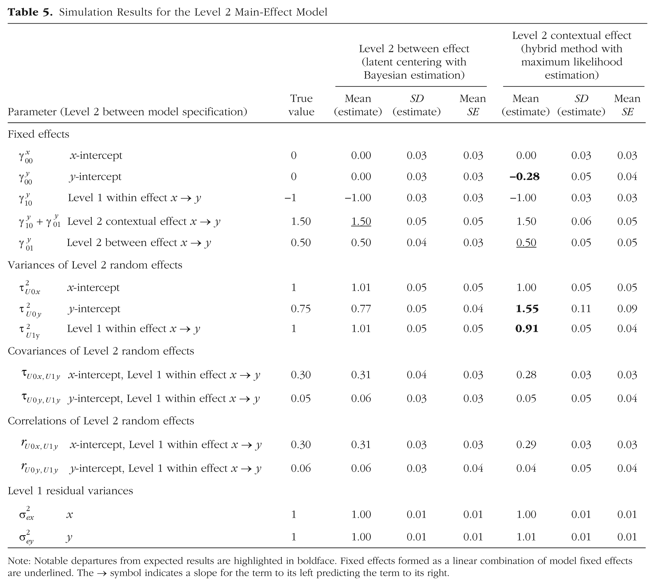
Note: Notable departures from expected results are highlighted in boldface. Fixed effects formed as a linear combination of model fixed effects are underlined. The → symbol indicates a slope for the term to its left predicting the term to its right.

At this point, the predictor fixed main effects were correctly estimated in each model. Notably, each model directly provided the correct Level 1 within effect (−1.00), but the models’ use of different versions of the Level 1 predictor resulted in different types of Level 2 fixed effects. That is, with latent centering and Bayesian estimation, the Level 2 fixed effect for ${\mathrm{\beta }}_{0b}^x$ β directly provided the Level 2 between main effect (0.50), whereas with the hybrid method and ML estimation, the same parameter became the Level 2 contextual main effect (1.50; Level 2 between effect – Level 1 within effect = 0.50 + 1.00 = 1.50).

These three fixed main effects—within, between, and contextual—are depicted in Figure 3a, in which the solid lines show predicted y_wb outcomes for three distinct Level 2 units (Level 2 predictor ${\mathrm{\beta }}_{0b}^x$ β values = −1, 0, or 1), each with three Level 1 units (Level 1 x_wb values = ±1 unit of their Level 2 ${\mathrm{\beta }}_{0b}^x$ β). First, the Level 1 within effect (−1.00) is given by the slope of the solid lines. The correct Level 1 within effect will always be provided by latent centering (because the Level 1 predictor is the x_wb residual, $e_{wb}^x$ , and thus contains only within-level variability); it can also be provided by the hybrid method (using the observed Level 1 predictor x_wb), but only after controlling for the Level 2 fixed effect. Second, the Level 2 between effect (0.50, as provided directly by latent centering) is given by the slope of the diagonal dashed line through the plots for the Level 2 units. Third, the Level 2 contextual effect (1.50) is the vertical distance associated with a 1-unit difference in Level 2 ${\mathrm{\beta }}_{0b}^x$ β (as provided directly by the hybrid method), holding constant the Level 1 x_wb value.

Fig. 3.

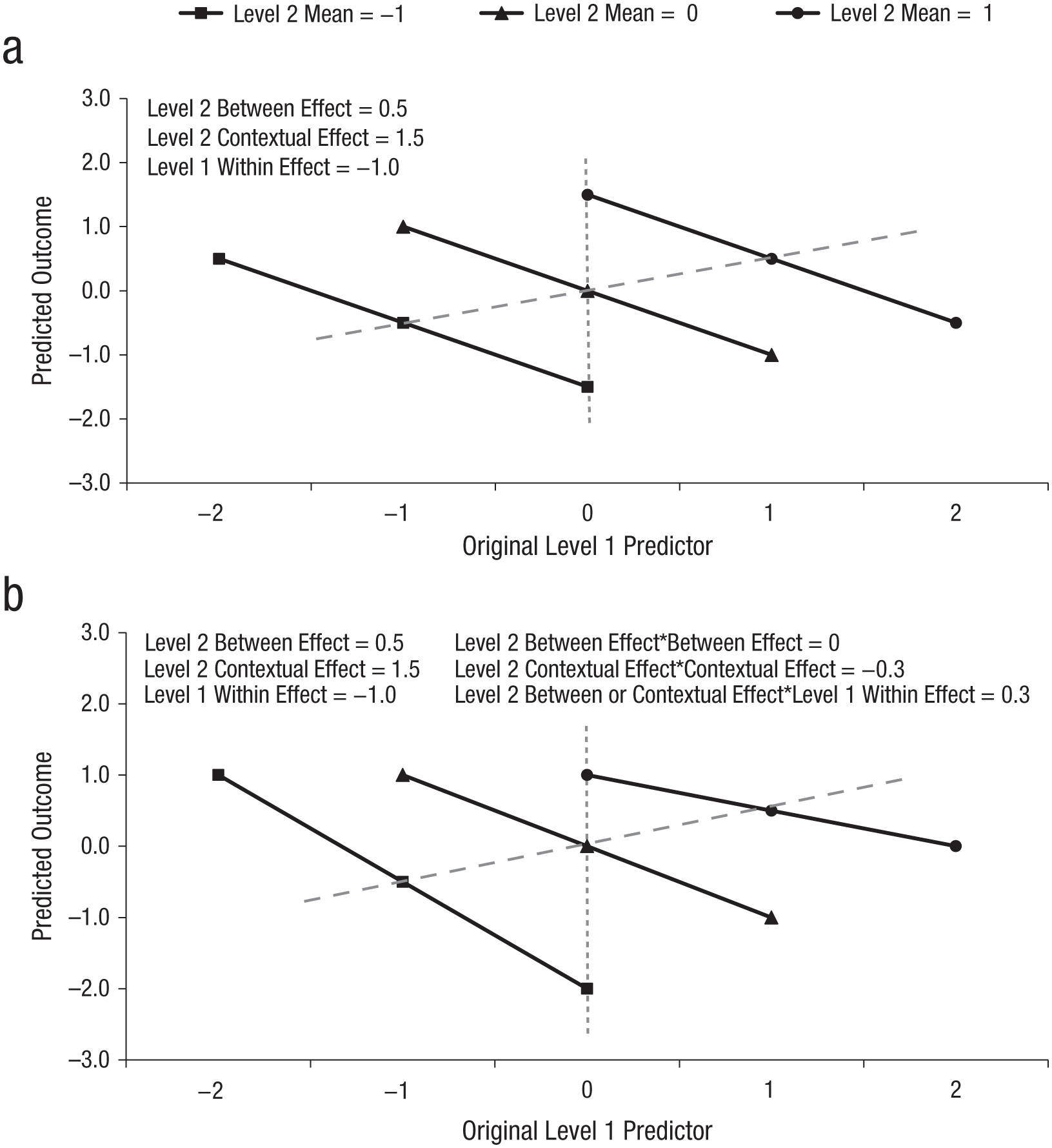
Simulation results: depiction of the analysis models including (a) a Level 2 main effect and (b) a Level 2 interaction. Solid black lines indicate Level 1 within effects, gray dashed diagonal lines indicate Level 2 between effects, and gray dotted vertical lines indicate Level 2 contextual effects.

Cross-level interaction model

To demonstrate how these two multivariate MLMs again lose their equivalence when a cross-level interaction is added, I added the Level 2 intercept for x_wb ( ${\mathrm{\beta }}_{0b}^x$ ) as a moderator of the Level 1 within effect of x_wb on y_wb, as shown in the model in the third panel of Table 3. Results are reported in Table 6. The new cross-level interaction, ${\mathrm{\gamma }}_{11}^y$ γ, had a slight downward bias relative to the population value (0.30) when the hybrid method and ML estimation were used (0.28), whereas the population value was recovered with latent centering and Bayesian estimation. The bias in the ML solution is actually a hint that this solution reflects a nonequivalent, misspecified model. That is, the cross-level interaction for the Level 2 latent predictor ${\mathrm{\beta }}_{0b}^x$ β was estimated with the latent Level 1 predictor $e_{wb}^x$ in the Bayesian solution, and thus provided the intended moderation of the within effect by ${\mathrm{\beta }}_{0b}^x$ . But in the solution using the hybrid method with ML, the same cross-level interaction was instead estimated with the observed Level 1 predictor x_wb, and so the solution provided a smushed interaction: It assigned the same amount of moderation by ${\mathrm{\beta }}_{0b}^x$ to both the Level 1 within and the Level 2 between effects of x_wb. Yet in the population model, the within-level moderation was 0.30, and the between-level moderation was 0 (given that it was not included in the generating model). The consequences of this smushed moderation (found only in the model using the hybrid method and ML estimation) are a too-small cross-level interaction ( ${\mathrm{\gamma }}_{11}^y$ = 0.28 instead of 0.30) and an inflated y_wb random intercept variance ( ${\mathrm{\tau }}_{U0y}^2$ ) relative to the corrected model, as discussed next.

Table 6.

Simulation Results for the Cross-Level Interaction Model

Parameter (Level 2 between model specification)		Level 2 between effect (latent centering with Bayesian estimation)			Level 2 contextual effect (hybrid method with maximum likelihood estimation)
	True value	Mean (estimate)	SD (estimate)	Mean SE	Mean (estimate)	SD (estimate)	Mean SE
Fixed effects
${\mathrm{\gamma }}_{00}^x$     x-intercept	0	0.01	0.03	0.03	0.00	0.03	0.03
${\mathrm{\gamma }}_{00}^y$     y-intercept	0	0.00	0.03	0.03	−0.28	0.05	0.04
${\mathrm{\gamma }}_{10}^y$     Level 1 within effect x → y	−1	−1.00	0.03	0.03	−1.00	0.03	0.03
${\mathrm{\gamma }}_{10}^y$ + ${\mathrm{\gamma }}_{01}^y$  Level 2 contextual effect x → y	1.50	1.50	0.05	0.04	1.50	0.06	0.05
${\mathrm{\gamma }}_{01}^y$ γ    Level 2 between effect x → y	0.50	0.50	0.04	0.03	0.50	0.05	0.05
${\mathrm{\gamma }}_{11}^y$     Level 1 Within Effect × Level 2  Between or Contextual Effect x → y	0.30	0.30	0.03	0.03	0.28	0.03	0.03
Variances of Level 2 random effects
${\mathrm{\tau }}_{U0x}^2$    x-intercept	1	1.01	0.05	0.04	1.00	0.05	0.05
${\mathrm{\tau }}_{U0y}^2$    y-intercept	0.75	0.77	0.05	0.05	1.55	0.11	0.09
${\mathrm{\tau }}_{U1y}^2$ τ    Level 1 within effect x → y	0.91	0.91	0.05	0.05	0.83	0.04	0.04
Covariance of Level 2 random effects
${\mathrm{\tau }}_{U0y,U1y}$   y-intercept, Level 1 within effect x → y	0.05	0.05	0.03	0.03	0.05	0.05	0.04
Correlation of Level 2 random effects
$r_{U0y,U1y}$    y-intercept, Level 1 within effect x → y	0.06	0.06	0.03	0.04	0.05	0.05	0.04
Level 1 residual variances
${\sigma }_{ex}^2$     x	1	1.00	0.01	0.01	1.00	0.01	0.01
${\sigma }_{ey}^2$     y	1	1.00	0.01	0.01	1.01	0.01	0.01

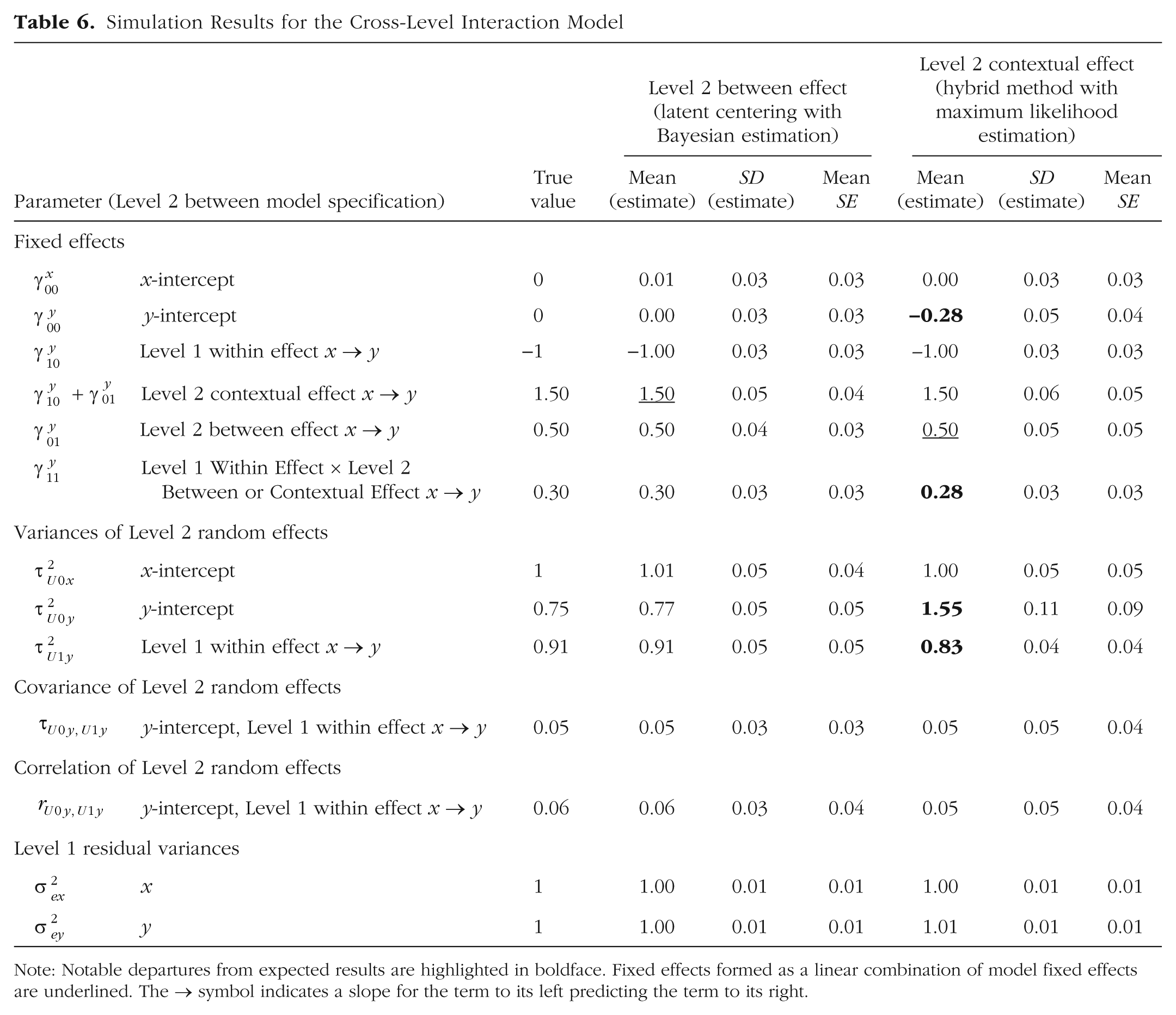
Note: Notable departures from expected results are highlighted in boldface. Fixed effects formed as a linear combination of model fixed effects are underlined. The → symbol indicates a slope for the term to its left predicting the term to its right.

Level 2 interaction model

In the last analysis model, I added a new Level 2 interaction to repair the previously misspecified cross-level interaction caused by using the hybrid method with ML estimation. As shown in the bottom panel of Table 3, a new observed Level 1 variable for squared x_wb (denoted xx_wb) was calculated in the data and included in the model. To unsmush the cross-level interaction, a fixed effect of the Level 2 intercept for xx_wb (denoted ${\mathrm{\beta }}_{0b}^{xx}$ ) was then added to predict the Level 2 intercept for y_wb, and covariances with $U_{0b}^{xx}$ were estimated with all the other random effects. Given that xx_wb was not needed as a predictor in the Level 1 model, covariances were estimated between its Level 1 residual and the residuals of the other Level 1 variables.

Results from this model are given in Table 7 and depicted in Figure 3b. First, let us consider the fixed main effects for the Level 1 and Level 2 x_wb predictors, which are now simple (conditional) effects given their interactions. Accordingly, the Level 1 within main effect (−1.00) is the slope across Level 1 units specifically when Level 2 ${\mathrm{\beta }}_{0b}^x$ β is 0, the Level 2 between main effect (0.50) is the slope of the line through the means of the Level 2 units, and the Level 2 contextual main effect (1.50) is the vertical distance associated with a 1-unit higher value of Level 2 ${\mathrm{\beta }}_{0b}^x$ (as provided directly with the hybrid method) when Level 1 x_wb is 0.

Table 7.

Simulation Results for the Level 2 Interaction Model

Parameter (Level 2 between model specification)		Level 2 between effect (latent centering with Bayesian estimation)			Level 2 contextual effect (hybrid method with maximum likelihood estimation)
	True value	Mean (estimate)	SD (estimate)	Mean SE	Mean (estimate)	SD (estimate)	Mean SE
Fixed effects
${\mathrm{\gamma }}_{00}^x$      x-intercept	0	0.00	0.03	0.03	0.00	0.03	0.03
${\mathrm{\gamma }}_{00}^{xx}$     x*x-intercept	2	2.00	0.05	0.05	2.00	0.05	0.05
${\mathrm{\gamma }}_{00}^y$     y-intercept	0	0.00	0.06	0.06	0.31	0.10	0.08
${\mathrm{\gamma }}_{10}^y$     Level 1 within effect x → y	−1	−1.00	0.03	0.03	−1.00	0.03	0.03
${\mathrm{\gamma }}_{10}^y$ + ${\mathrm{\gamma }}_{01}^y$  Level 2 contextual effect x → y	1.50	1.50	0.05	0.05	1.51	0.06	0.05
${\mathrm{\gamma }}_{01}^y$     Level 2 between effect x → y	0.50	0.50	0.04	0.03	0.51	0.05	0.05
${\mathrm{\gamma }}_{11}^y$     Level 1 Within Effect × Level 2 Between or  Contextual Effect x → y	0.30	0.30	0.04	0.04	0.30	0.04	0.03
${\mathrm{\gamma }}_{02}^y$ – ${\mathrm{\gamma }}_{11}^y$ Level 2 contextual effect x*x → y	−0.30	−0.30	0.05	0.04	−0.30	0.05	0.04
${\mathrm{\gamma }}_{02}^y$     Level 2 between effect x*x → y	0	0.00	0.02	0.03	0.00	0.04	0.05
Variances of Level 2 random effects
${\mathrm{\tau }}_{U0x}^2$ τ   x-intercept	1	1.00	0.05	0.05	1.00	0.05	0.05
${\mathrm{\tau }}_{U0xx}^2$    x*x-intercept	2	2.00	0.25	0.11	2.01	0.25	0.11
${\mathrm{\tau }}_{U0y}^2$    y-intercept	0.75	0.77	0.05	0.05	1.39	0.09	0.08
${\mathrm{\tau }}_{U1y}^2$   Level 1 within effect x → y	0.91	0.92	0.05	0.05	0.83	0.04	0.04
Covariances of Level 2 random effects
${\mathrm{\tau }}_{U0y,U1y}$  y-intercept, Level 1 within effect x → y	0.05	0.06	0.03	0.03	0.05	0.05	0.04
${\mathrm{\tau }}_{U0x,U0xx}$   x-intercept, x*x-intercept	0	0.01	0.12	0.05	0.01	0.12	0.05
${\mathrm{\tau }}_{U0xx,U1y}$ x*x-intercept, Level 1 within effect x → y	0	−0.01	0.05	0.05	0.00	0.04	0.05
Correlations of Level 2 random effects
$r_{U0y,U1y}$  y-intercept, Level 1 within effect x → y	0.06	0.07	0.03	0.04	0.05	0.05	0.04
$r_{U0x,U0xx}$ x-intercept, x*x-intercept	0	0.01	0.08	0.04	0.01	0.08	0.04
$r_{U0xx,U1y}$ x*x-intercept, Level 1 within effect x → y	0	−0.01	0.03	0.04	0.00	0.03	0.04
Level 1 residual variances
${\sigma }_{ex}^2$    x	1	1.00	0.01	0.01	1.00	0.01	0.01
${\sigma }_{exx}^2$     x*x	6	6.02	0.24	0.07	6.01	0.24	0.07
${\sigma }_{ey}^2$    y	1	1.00	0.01	0.01	1.01	0.01	0.01
Covariances of Level 1 residuals
${\sigma }_{exx,ex}^2$   x*x, x	0	0.01	0.08	0.02	0.01	0.08	0.02
${\sigma }_{exx,ey}^2$   x*x, y	0	0.01	0.05	0.04	0.00	0.04	0.04

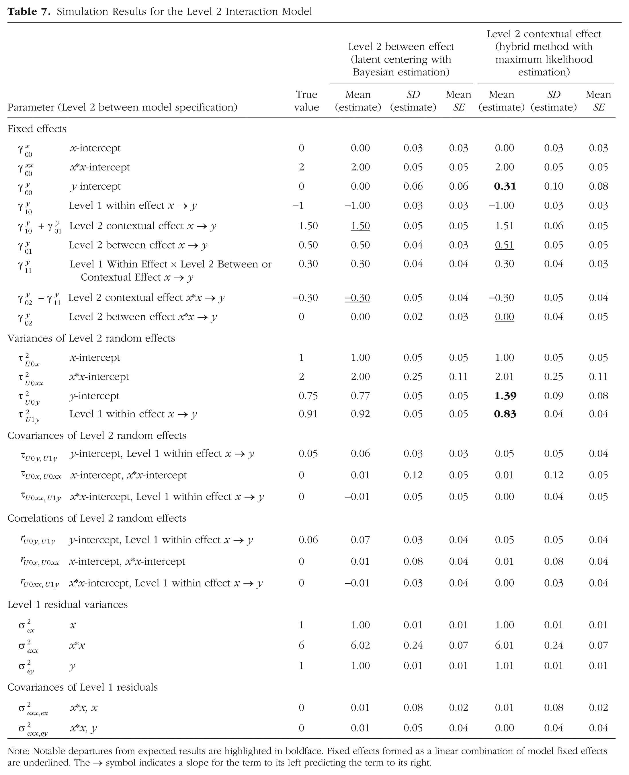
Note: Notable departures from expected results are highlighted in boldface. Fixed effects formed as a linear combination of model fixed effects are underlined. The → symbol indicates a slope for the term to its left predicting the term to its right.

Now let us consider the impact of the new Level 2 interaction of ${\mathrm{\beta }}_{0b}^{xx}$ ( ${\mathrm{\gamma }}_{02}^y$ ), which served to allow the moderation by ${\mathrm{\beta }}_{0b}^x$ to differ across levels when the hybrid method with ML estimation was used. As expected, unsmushing the cross-level interaction reduced the too-high Level 2 random intercept variance ( ${\mathrm{\tau }}_{U0y}^2$ ), and the Level 1 within moderation by ${\mathrm{\beta }}_{0b}^x$ was recovered accurately by the cross-level interaction ( ${\mathrm{\beta }}_{11}^y$ γ). This moderation is shown in Figure 3b by the change in the Level 1 within slope across Level 2 units: The Level 1 within slope was less positive by 0.30 for every 1-unit higher Level 2 ${\mathrm{\beta }}_{0b}^x$ .

As we saw with the Level 2 main effects, the interpretation of the Level 2 interaction ( ${\mathrm{\gamma }}_{02}^y$ ) differs between the Bayesian and ML solutions as a result of their differing Level 1 predictors. When latent centering with Bayesian estimation is used, ${\mathrm{\gamma }}_{02}^y$ is the Level 2 between moderation, which was 0 in the population. This is shown in Figure 3b by the equal distance between Level 2 units at their means; the linear slope of the diagonal dashed line as ${\mathrm{\beta }}_{0b}^x$ β increases indicates that there is no between-level interaction. In contrast, when the hybrid method with ML estimation is used, ${\mathrm{\gamma }}_{02}^y$ is the Level 2 contextual moderation (−0.30 in the present case) instead. In Figure 3b, this contextual moderation is shown by the unequal distance between Level 2 units along the vertical dotted line. That is, holding Level 1 x_wb constant, the vertical distance between Level 2 units becomes smaller by 0.30 for each 1-unit higher value of Level 2 ${\mathrm{\beta }}_{0b}^x$ . Said differently, the Level 2 between moderation ( ${\mathrm{\gamma }}_{02}^y$ = 0, given by latent centering with Bayesian estimation) is less positive by the Level 2 contextual moderation ( ${\mathrm{\gamma }}_{02}^y$ = −0.30, given by the hybrid method with ML estimation) than the Level 1 within moderation ( ${\mathrm{\gamma }}_{11}^y$ = 0.30, given in both solutions after allowing level-specific moderation).

Multivariate MLMs as Single-Level SEMs

In addition to phrasing multivariate MLMs as multilevel SEMs, as just demonstrated, it is possible (to some extent) to estimate them using standard software for single-level structural equation modeling. The key to doing so lies in understanding the data structure used by each type of model. As in univariate MLMs, each Level 1 unit in a multilevel SEM has its own data row. For instance, in my simulation of 15 Level 1 units within each of 1,000 Level 2 units, a multilevel SEM data structure required 15,000 rows of three variables: Level 2 unit ID, Level 1 x_wb, and Level 1 y_wb. In contrast, in single-level SEMs, all data for each Level 2 unit are contained in a single row, in which the Level 1 observations are stored as separate variables. Given a maximum of 15 Level 1 units per Level 2 unit, the data structure required for a single-level SEM would have 1,000 rows of 31 variables: Level 2 unit ID, 15 variables for Level 1 x_wb (as x1–x15), and 15 variables for Level 1 y_wb (as y1–y15). (Level 2 units with fewer than 15 Level 1 units would thus have missing data for some of their observed variables.)

In a single-level SEM, the Level 2 model is defined through latent factors that predict the Level 1 observed variables. To mimic the multivariate MLMs estimated for my simulated data, one latent “intercept” factor is defined for x1 through x15, a second is defined for y1 through y15, all factor loadings are fixed to 1, all intercepts for the observed variables are fixed to 0, and the residual variances of the observed variables are held equal. The latent factor means are the fixed intercepts, and the latent factor variances are the Level 2 random intercept variances. The Level 1 model in a single-level SEM is defined using the residuals of the Level 1 observed variables, which contain only within-level variability after controlling for the latent factors. This specification, referred to in Table 1 as residual direct, is equivalent to the hybrid method of multilevel structural equation modeling with ML estimation in Mplus. A Level 1 fixed effect can be estimated by specifying direct paths (all constrained to be equal) between the corresponding residuals of the Level 1 observed variables using the latent placeholder syntax, in which the PON command creates pairwise regressions (e.g., s | y1-y15 PON x1-x15;). A direct path between the latent factors then provides the Level 2 contextual fixed effect.

To illustrate this method, I estimated the same population and analysis models just described as multilevel SEMs using the same simulated data, but this time I used single-level SEM syntax with ML estimation. The results are provided in the Supplemental Material. As expected, the results were exactly the same as those for the multilevel SEMs with ML estimation (as reported in Tables 4–7). It was not possible to estimate the same single-level SEMs using Bayesian estimation given the Level 2 random slope for the Level 1 effect.

Another variant of model specification using single-level SEMs uses structured residuals (see Table 1). In this approach, as described by Curran, Howard, Bainter, Lane, and McGinley (2014), the residuals of the Level 1 observed variables are first transferred to new latent variables, between which Level 1 fixed effects are then specified. When a Level 1 effect is specified through the new residual latent variables (which each contain only Level 1 within-level variability), a direct path between the latent variables provides the Level 2 between effect instead of the Level 2 contextual effect. However, it currently is not possible to use structured residuals to estimate random slope variances for Level 1 effects (through the Level 1 placeholder syntax).

Summary and Recommendations

In this article, I have aimed to explain and illustrate how effects in MLMs should be interpreted, depending on the analyst’s choices (as summarized in Table 1). Given the many nuances involved in this intersection of model specification and software implementation, it can be easy to lose sight of the bigger picture. To that end, I conclude with some practical strategies that can help analysts avoid two primary mistakes that could mar an otherwise meaningful multilevel analysis.

Mistake #1: failing to differentiate fixed effects at different levels of analysis

The first mistake, referred to here and elsewhere as the problem of smushing (Hoffman, 2015), is failing to differentiate the effects of a predictor at different levels of analysis. Although in the current context of two-level models only Level 1 predictors are at risk, smushing can happen to any predictor measured below the top level of the model (e.g., Level 2 predictors in three-level models). In this article’s examples, smushing referred to the problem of fitting a single fixed effect of a Level 1 predictor that had variability at both Level 1 and Level 2, such that the single fixed effect constrained the Level 1 within and Level 2 between effects to be the same. Although this problem has most often been described with respect to lower-level main effects, smushing can also occur when interactions with lower-level predictors are estimated. Fortunately, avoiding the mistake of smushing can become more straightforward by following two steps.

The first step is the easier one: Ascertain the levels at which each lower-level predictor contains variability. For predictors with plausibly normal distributions, this can be done using the empty-means model in Equation 1; for other types of predictors (e.g., ordinal or count variables), a more appropriate generalized MLM variant should be used to fit an empty-means model. Such inspection of variability is an important first step because the presence of level-specific variance is a logical precursor to finding level-specific effects (and thus possible differences between effects at different levels). In addition to level-specific intercept variability, possible level-specific slope variability should be considered. That is, in longitudinal designs, one should test whether time-varying predictors also have between-level variation in the effects of time; between-level variation in the slope of important lower-level predictors can also be relevant in some clustered designs. The bottom line is that a full consideration of how a predictor relates to an outcome includes considering the potential effect of each source of variation in the predictor.

The second step is to ensure that each predictor’s effect is included at every level of the model at which it contains at least some variability. This step can be much more complicated, because one must decide how to represent these level-specific sources of variability as predictors in the model. In this article, I have described the two primary approaches for representing predictor variables: using univariate MLMs and using multivariate MLMs.

When higher-level variability in lower-level predictors is found only in the intercept, one could represent that intercept variability with an observed predictor variable—the mean across lower-level units (e.g., a Level 2 mean ${\overline{x}}_b$ across its Level 1 x_wb values). Variability at each lower level could then be represented by observed predictor variables as well. This is the univariate MLM approach, which has the advantage of lending itself to many available software options (the Supplemental Material provides Mplus code mapping onto the univariate MLM examples from Equations 1 through 7). But univariate MLMs also have potential disadvantages, most notably with respect to the deletion of cases that have missing model predictors (i.e., variables that are not included in the model likelihood), as well as potential introduction of bias in the higher-level fixed effects (see Lüdtke et al., 2008; Preacher et al., 2011, 2016).

Alternatively, one can treat the lower-level predictor as an outcome (i.e., include it as part of the model likelihood), which then allows its model-estimated variance components to become level-specific latent predictor variables. This is the multivariate MLM approach, which is preferred whenever there is higher-level variability in both lower-level slopes and intercepts (such as when a time-varying predictor shows between-level differences in both the intercept and change over time). As illustrated in the Supplemental Material, multivariate MLMs can be estimated using software for multilevel SEMs and, to a lesser extent, software for single-level SEMs. Although multivariate MLMs can overcome the limitations inherent in univariate MLMs (cases that are missing predictors are not deleted when those predictors are treated as outcomes; bias in higher-level fixed effects is reduced through the use of latent higher-level variables), treating predictors as outcomes means that distributional assumptions for them are invoked. If the typical default distribution—multivariate normal at each level of the model—is not appropriate, then fitting a generalized version of a multivariate MLM (i.e., using nonlinear link functions and nonnormal conditional distributions to predict model outcomes) is possible but can result in even more complexity in estimation (which is already higher in multivariate than in univariate MLMs).

Mistake #2: failing to differentiate types of higher-level effects

Once your model results are generated, it is time to avoid the second mistake: incorrectly interpreting Level 2 contextual effects as Level 2 between effects (or vice versa). To avoid this confusion, it is imperative to determine whether the lower-level predictor variables in your model are level-specific or not, as this distinction dictates which kind of higher-level effects necessarily result. Distinguishing level-specific from non-level-specific predictors should be easy in the case of a univariate MLM, given that you will know exactly which observed predictors you have included. In the case of a multivariate MLM, you should thoroughly consult the software documentation to ensure that you understand the approach invoked by your choices for model specification and estimation (see Table 1 for information on the effects provided when Mplus 8.1+ is used). This article’s Supplemental Material can also aid diagnosis: By estimating the same models using a single simulated data set (as provided in the Supplemental Material), you can check your understanding of the procedures invoked in other software by verifying whether your results match those of the higher-level contextual or between effects (as found in the Mplus output also provided in the Supplemental Material). Table 2 shows how either higher-level fixed effect can be approximated from the other (given that contextual effect = between effect – within effect; for an extension to other interaction models, see Hoffman, 2015).

The first type of lower-level predictors retain their variation at higher levels. This is the case for constant-centered observed predictors in univariate MLMs, as well as for observed predictors in multivariate MLMs when the Mplus hybrid method (or an analogous method) is used. In such cases, the lower-level predictor will have its correct, level-specific, unsmushed effects only after inclusion of its effects at the higher levels of the model at which it also contains variance. Those higher-level effects will then be contextual, indicating the impact on the outcome of a 1-unit difference in the higher-level predictor after controlling for the absolute value of the corresponding lower-level predictor.

The second type of lower-level predictors contain variation at a single level only. These level-specific predictors result when observed predictors are variable centered in univariate MLMs or when they are latent centered in multivariate MLMs (or when a multivariate MLM uses analogous model-based variance partitioning). In addition, predictors at the highest level of the model are level-specific by definition. The effects arising from level-specific predictors are often easier to understand: If a variable has variance at only one level, then its effect can pertain only to that specific level. Consequently, there is no need to worry that a lower-level effect has been smushed, and the predictor’s higher-level effect will be a between effect—the impact on the outcome of a 1-unit difference in the predictor, not controlling for the absolute value of the corresponding lower-level predictor.

The consequences of confusing higher-level contextual and between effects will depend on the exact configuration of these fixed effects, but let us consider two example scenarios involving two-level models. Figure 4 illustrates each scenario.

Fig. 4.

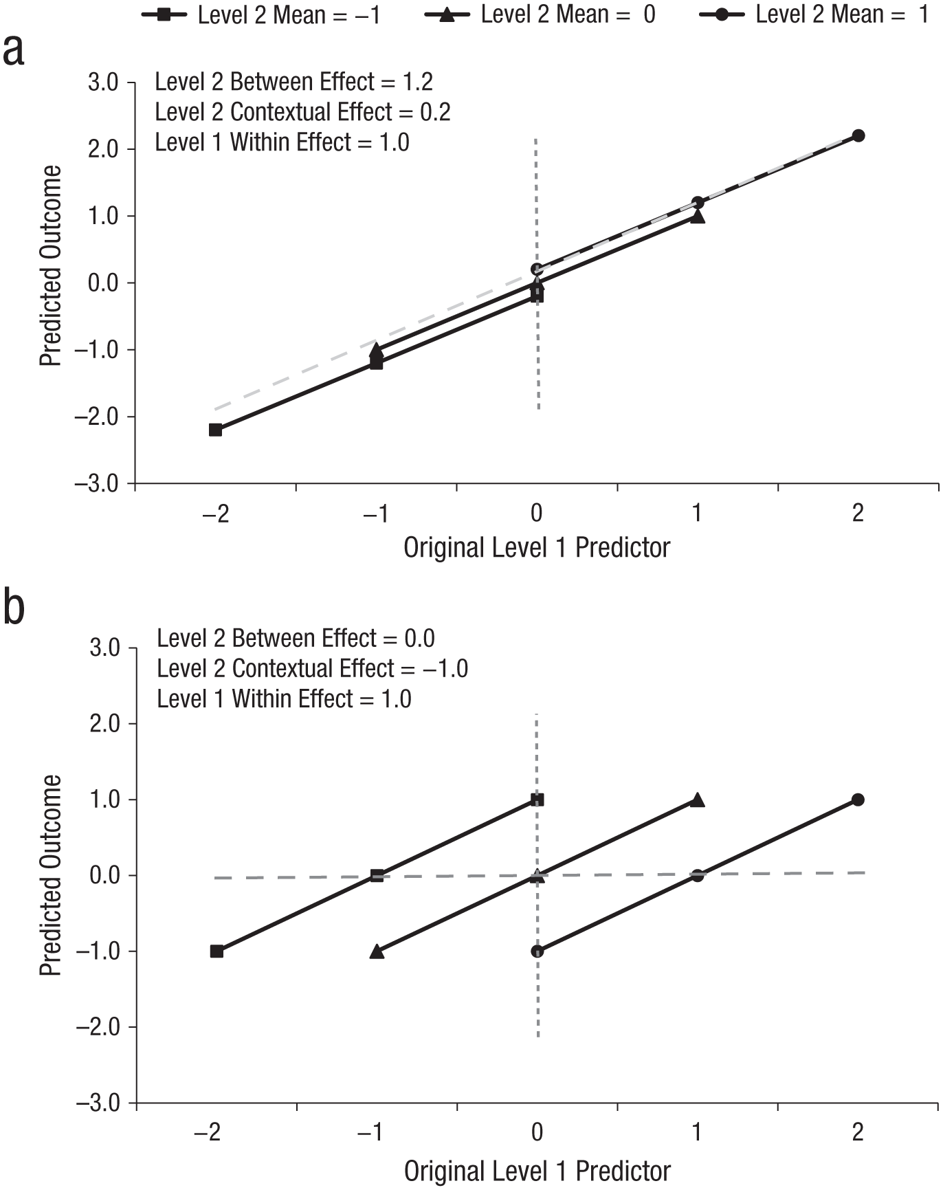
Depiction of hypothetical scenarios in which confusing higher-level contextual and between effects will result in misinterpretation: (a) a scenario with positive Level 1 within and Level 2 between effects and (b) a scenario with a positive Level 1 within effect and a zero Level 2 between effect. In each panel, the Level 1 within effects are the slopes of the solid lines (one for each of the three Level 2 units), the Level 2 between effect is the slope of the diagonal dashed line through the means of the Level 2 units, and the Level 2 contextual effect is shown by the distance between Level 2 units along the vertical dotted line.

As depicted in Figure 4a, the Level 1 within and Level 2 between effects in the first scenario are each significantly positive, such that having more of the predictor than others in the same Level 2 unit (Level 1 within effect of 1.0) and belonging to a Level 2 unit with more of the predictor than other units on average (Level 2 between effect of 1.2) both result in higher outcomes. Given Level 1 within and Level 2 between effects of similar magnitudes, the Level 2 contextual effect (which tests their difference, which is 0.2 in the present case) may not be significant. In this kind of scenario, if an analyst thinks that a nonsignificant Level 2 contextual effect is the Level 2 between effect, the analyst would conclude that belonging to a Level 2 unit with more of the predictor than other units on average does not matter, which is not true. Instead, the correct conclusion is that the advantage afforded by this Level 2 unit’s higher mean does not matter incrementally after considering that its Level 1 units had more of the predictor to begin with. In other words, at the same absolute level of the Level 1 predictor, there is no difference in the outcome between Level 2 units (as shown by the vertical distance between the lines in Fig. 4a).

Alternatively, consider the pairing of the same significantly positive Level 1 within effect with a zero Level 2 between effect, as depicted in Figure 4b. Now the Level 2 contextual effect must be negative, given that the contextual effect is equal to the between effect minus the within effect. In this case, an analyst who mistakes the obtained Level 2 contextual effect for a Level 2 between effect would conclude that belonging to a Level 2 unit with more of the predictor than other units on average results in lower outcomes, whereas in reality it makes no difference (i.e., the slope through the Level 2 unit means in Fig. 4b is flat). Instead, a comparison of Level 1 units with the same absolute amount of the Level 1 predictor (i.e., Level 1 units at the same point on the x-axis) shows that outcomes are lower for Level 1 units from Level 2 units that have more of the predictor on average (but have low levels of the predictor relative to their Level 2 unit) than for Level 1 units from Level 2 units that have less of the predictor on average (but have high levels of the predictor relative to their Level 2 unit). Situations in which Level 2 contextual and between effects differ can be tricky to summarize, but it should always be helpful to start by clarifying the direction, magnitude, and significance for each type of effect.

Conclusion

The power of univariate and multivariate multilevel modeling for addressing complex questions at multiple levels of sampling offers great potential for facilitating empirical research in many areas. But with great power comes great responsibility, and I hope the present work will help multilevel analysts feel more comfortable in understanding how the choices they make will translate into different model interpretations and real-world explanations.

Supplemental Material

Hoffman_Final_Open_Practices_Disclosure – Supplemental material for On the Interpretation of Parameters in Multivariate Multilevel Models Across Different Combinations of Model Specification and Estimation

Supplemental material, Hoffman_Final_Open_Practices_Disclosure for On the Interpretation of Parameters in Multivariate Multilevel Models Across Different Combinations of Model Specification and Estimation by Lesa Hoffman in Advances in Methods and Practices in Psychological Science

Supplemental Material

Hoffman_Multivariate_MLM_Supplemental_Files_(9) – Supplemental material for On the Interpretation of Parameters in Multivariate Multilevel Models Across Different Combinations of Model Specification and Estimation

Supplemental material, Hoffman_Multivariate_MLM_Supplemental_Files_(9) for On the Interpretation of Parameters in Multivariate Multilevel Models Across Different Combinations of Model Specification and Estimation by Lesa Hoffman in Advances in Methods and Practices in Psychological Science