Sage Journals: Discover world-class research

Abstract

The percentile bootstrap is the Swiss Army knife of statistics: It is a nonparametric method based on data-driven simulations. It can be applied to many statistical problems, as a substitute to standard parametric approaches, or in situations for which parametric methods do not exist. In this Tutorial, we cover R code to implement the percentile bootstrap to make inferences about central tendency (e.g., means and trimmed means) and spread in a one-sample example and in an example comparing two independent groups. For each example, we explain how to derive a bootstrap distribution and how to get a confidence interval and a p value from that distribution. We also demonstrate how to run a simulation to assess the behavior of the bootstrap. For some purposes, such as making inferences about the mean, the bootstrap performs poorly. But for other purposes, it is the only known method that works well over a broad range of situations. More broadly, combining the percentile bootstrap with robust estimators (i.e., estimators that are not overly sensitive to outliers) can help users gain a deeper understanding of their data than they would using conventional methods.

Keywords

bootstrap confidence interval correlation R simulation trimmed mean median reaction time skewness group comparison open materials

The main idea behind the bootstrap is that in some situations, it is better to make inferences about a population parameter using only the data at hand, without making assumptions about underlying distributions. For instance, the t test is based on the assumption that the t statistic has a certain sampling distribution, given some assumptions about the population.¹ However, when these assumptions are wrong, the t test does not behave as expected, which potentially leads to increased numbers of false positives and lack of statistical power. With the bootstrap, one does not make such assumptions, but instead uses the data to estimate sampling distributions using computer-based simulations, sampling from the data with replacement.

Many bootstrap techniques have been developed to address a large variety of statistical problems, and we refer interested readers to reviews, books, and tutorials on this vast topic (e.g., Efron & Hastie, 2016; Efron & Tibshirani, 1994; Hesterberg, 2015b; Rousselet et al., 2019; Wilcox, 2017). Without going into the details, for the purpose of this Tutorial we focus on bootstrapping as an important statistical concept and use the percentile bootstrap, the simplest form of bootstrap, for illustration. This method has been shown to work in a large variety of situations, and its simplicity is ideal for learning how the bootstrap works. First, we explain how the percentile bootstrap is implemented in base R (R Core Team, 2020), before covering the calculation of confidence intervals and p values, and how to perform group comparisons (see our companion R Notebook on GitHub, at https://github.com/GRousselet/bootsteps). For an accessible introduction to R, we recommend several print books (Crawley, 2012; Dalgaard, 2008; Wickham & Grolemund, 2017), as well as the free online R for Data Science (Grolemund & Wickham, n.d.). Bootstrap functions are available in many R packages, some of which are listed in Table 1. All these packages differ in their implementations. For instance, the popular boot package (Tibshirani & Leisch, 2019) provides a generic function that can handle many situations, but it requires users to write functions, which is impractical for R beginners. In this Tutorial, we focus on low-level R implementation, to give users a concrete understanding of the bootstrap’s mechanics. In addition, the companion R Notebook demonstrates how to use functions from Wilcox (2017) and from the boot package.

Table 1.

Examples of R Packages Containing Bootstrap Functions

R package	Link	Additional reference
bootstrap	https://CRAN.R-project.org/package=bootstrap (Tibshirani & Leisch, 2019)	Efron and Tibshirani (1994)
boot	https://CRAN.R-project.org/package=boot (Canty & Ripley, 2020)	Davison and Hinkley (1997)
simpleboot	https://CRAN.R-project.org/package=simpleboot (Peng, 2019)
WRS2	https://CRAN.R-project.org/package=WRS2 (Mair & Wilcox, 2020b)	Mair and Wilcox (2020a)
resample	https://CRAN.R-project.org/package=resample (Hesterberg, 2015a)	Hesterberg (2015b)
car (Boot)	https://CRAN.R-project.org/package=car (Fox & Weisberg, 2019a)	Fox and Weisberg (2019b)
nlstools (nlsBoot)	https://CRAN.R-project.org/package=nlstools (Baty & Delignette-Muller, 2015)	Baty et al. (2015)
dabestr	https://CRAN.R-project.org/package=dabestr (Ho & Tumkaya, 2020)	Ho et al. (2019)
rogme	https://github.com/GRousselet/rogme (Rousselet & Wilcox, 2020b)	Rousselet et al. (2017)

Note: For packages not focused on bootstrap methods, example bootstrap functions are listed in parentheses.

Disclosures

All the figures and analyses presented in this Tutorial can be reproduced using a notebook in the R programming language (R Core Team, 2020) that we have made available on OSF (https://osf.io/dvuze/). Novice R users will probably find the GitHub version of the code easier to use (https://github.com/GRousselet/bootsteps). Using the R Notebook also requires the free and user-friendly RStudio interface (RStudio Team, 2020). The figures were created using the ggplot2 package (Wickham, 2016).

Bootstrap Implementation

The core mechanism of the bootstrap is sampling with replacement, which is equivalent to simulating experiments using only the data at hand. Let us say we have a sample that is a sequence of integers:



samp
[1] 1 2 3 4 5 6

The last line, starting with [1], indicates an output in the R console. We can create this sequence using these commands in R:



n <- 6 # sample size
samp <- c(1:n)

To make bootstrap inferences, we sample with replacement from that sequence using the sample() function. That is the engine under the hood of any bootstrap technique. The following code will generate our first bootstrap sample:



set.seed(21) # for reproducible
 results
sample(samp, size = n, replace =
 TRUE) # sample with replacement
[1] 1 3 1 2 5 3

The function set.seed() is used to determine the starting point of the random-number generator used by the sample() function. The number 21 has no particular meaning; it just ensures that different users of the same lines of code will get the same pseudorandom outcome (providing they use the same version of R). Typing some other value in this function will give a different result. We recommend setting the seed to some value when the code is distributed as part of a reproducibility package, for instance, as supplementary information accompanying a research article. Because the bootstrap involves random sampling, it is also important to check that the bootstrap results are consistent across multiple seeds. This can be done by commenting out (adding # at the start of the line) or deleting the set.seed call and then running the same chunk several times. If the results differ substantially across repeated calls to the same bootstrap code or function, the number of bootstrap samples should probably be increased (see discussion in Hesterberg, 2015b).

The three arguments of the sample function are used to define a vector of values to sample from, the size of each sample, and whether one wants to sample with or without replacement. For the percentile bootstrap, the size of the samples is always equal to the size of the data being sampled from, and sampling is always with replacement.

If we run the sample command again, we obtain another bootstrap sample:



[1] 3 4 2 6 6 6

And running the command another time, we obtain a third sample:



[1] 3 6 2 3 4 5

We could also generate our three bootstrap samples in one go:



nboot <- 3
matrix(sample(samp, size = n*nboot,
 replace = TRUE), nrow = nboot, byrow =
 TRUE)
    [,1] [,2] [,3] [,4] [,5] [,6]
[1,]   1   3   1   2   5   3
[2,]   3   4   2   6   6   6
[3,]   3   6   2   3   4   5

As is apparent from these three examples, in a bootstrap sample, some observations are sampled more than once, and others are not sampled at all. So each bootstrap sample is like a virtual experiment in which one draws random observations from the original sample. That is, with the bootstrap, one estimates from the data what it would be like to perform many experiments using the same population. This is sometimes called the plug-in principle (Efron, 2003).

How will we use the bootstrap samples? It might be tempting to use them to make inferences about the mean of our sample by asking what are the plausible population means compatible with our data, without making any parametric assumptions. To answer this question, we compute the mean for each bootstrap sample. This can be done using a for loop. Although for loops can be avoided to write more compact code, they are very practical in many situations, and they make the code easier to read. Also, note that in R, as in Python (van Rossum & Drake, 2009), indexing is done using square brackets (e.g. boot.m[B]), whereas some other languages (e.g., MATLAB; Higham & Higham, 2016) use parentheses. We now generate 1,000 bootstrap samples using a for loop:



nboot <- 1000 # number of bootstrap
 samples
# declare vector of results
boot.m <- vector(mode = "numeric",
 length = nboot)
for(B in 1:nboot){ # bootstrap loop
boot.samp <- sample(samp, size = n,
 replace = TRUE) # sample with
 replacement
boot.m[B] <- mean(boot.samp) # save
 bootstrap means
}

The loop could be replaced by one line of code in which all bootstrap samples are generated at once (size = n*nboot), the results are reshaped as a matrix, and the apply() function is used to compute the mean for each row of the matrix of bootstrap samples:



boot.m <- apply(matrix(sample(samp,
 size = n*nboot, replace = TRUE),
 nrow = nboot), 1, mean)

The lollipop chart in Figure 1 illustrates the first 50 bootstrap means for this example, in the order in which they were sampled. The bootstrap means randomly fluctuate around the sample mean. They represent the means we could expect if we were to repeat the same experiment many times, given that we can sample only from the data at hand. Because we bootstrapped a very small sample of integer values, the bootstrap means take only a small number of unique values—25 exactly. We come back to this point later on.

Fig. 1.

The first 50 bootstrap means for our example. The thick gray horizontal line marks the sample mean (3.5).

All the bootstrap means can be illustrated using a density plot, which is like a smooth histogram that shows the relative probability of observing different bootstrap means (Fig. 2). This bootstrap distribution is an estimate of the sampling distribution of the mean (plug-in principle).

Fig. 2.

Density plot of 1,000 bootstrap means for our example. The thick gray vertical line marks the sample mean.

Bootstrap confidence interval

From this bootstrap distribution, we can derive a confidence interval as follows:



alpha <- 0.05
ci <- quantile(boot.m, probs =
 c(alpha/2, 1-alpha/2))
round(ci, digits = 3)
2.5% 97.5%
2.17 4.83

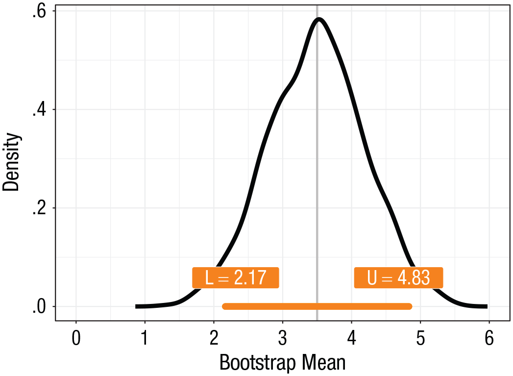
In the code, we set alpha to .05 to obtain a 95% confidence interval. The confidence interval bounds are defined as the alpha/2 (.025) and 1-alpha/2 (.975) quantiles of the bootstrap distribution. These quantiles of the bootstrapped means correspond to the definition of the confidence interval: an interval that captures the mean in 1 – alpha cases in the long run. The resulting confidence interval is [2.17, 4.83], which is illustrated in Figure 3. Note that the quantile() function offers nine options for estimating the quantiles; here we used the default, quantile(x, type = 7). In certain situations, such as when the bootstrap estimates take only a limited number of values (Hesterberg, 2015b), quantile(x, type = 6) is recommended.

Fig. 3.

The bootstrap 95% confidence interval for our example. The interval is depicted as an orange bar, with labels for the values of the lower (L) and upper (U) bounds.

Bootstrap p value

To define a p value, we need a null value, which in our example is 2.5 (Fig. 4). Half of the p value (or a one-sided p value) is the smaller of the proportion of bootstrap means to the left of the null value and the proportion of bootstrap means to the right of the null value. In our example, the smaller proportion is to the left of the null value. To obtain the bootstrap p value (or two-sided p value), we multiply that value by 2.

Fig. 4.

The bootstrap p value for our example, given that the null value of the population mean is 2.5.

Using code, the p value is obtained this way:



null.value <- 2.5 # null value for
 hypothesis testing
half.pval <- mean(boot.m > null.
 value) +.5*mean(boot.m == null.
 value)
pval <- 2*min(c(half.pval,1-half.
 pval)) # P value = 0.155
pval
[1] 0.155

First we set the null value, and then we compute the proportions corresponding to the shaded areas in Figure 4. Note how the p value calculation also considers borderline cases in which the bootstrap means are exactly equal to the null value. This is done to handle the type of situation we are dealing with in our simple example: The bootstrap means of a small number of integer values can take only a limited number of unique values (Fig. 1). A similar situation occurs when quantiles (e.g., medians) are estimated from relatively small sample sizes or when results have been rounded.

After computing the smallest proportion (area) in the density plot, we multiply it by 2 to obtain the p value (which is .155 in our example). Intuitively, the bootstrap p value reflects how deeply the null value is nested inside the bootstrap distribution; in other words, the bootstrap p value is related to how close the null value is to the center of the bootstrap distribution. If the null value is completely outside the bootstrap distribution, then the p value is 0; if the null value is exactly at the center of the bootstrap distribution, then the p value is 1.

Confidence interval coverage and robust estimation

It is important to consider how the percentile bootstrap performs in various situations and how it compares with other methods. This topic has received a lot of attention in many books and articles (see the introduction and the Conclusion section), and we cannot do it justice here. However, it is worth exploring a simple situation to learn a bit more about the percentile bootstrap in particular, and how to set up simulations in general (interested readers can find much more information about conducting simulation studies in Morris et al., 2019). Let us consider a simple simulation to check the probability coverage of confidence interval methods; that is, we want to find out how often 95% confidence intervals (from many repeated experiments) include the true population mean. By definition, if we compute 95% confidence intervals, about 95% of such intervals should contain the population mean (Greenland et al., 2016). We set up our simulation using this code:



set.seed(666) # reproducible results
nsim <- 5000 # simulation iterations
nsamp <- 30 # sample size
alpha <- 0.05 # alpha level
nboot <- 2000 # number of bootstrap
 samples
pop <- rlnorm(1000000) # define lognormal population
pop.m <- mean(pop) # population mean
ptrim <- 0.2 # proportion of trimming
pop.tm <- mean(pop, trim = ptrim)
 # population 20% trimmed mean

The simulation has 5,000 iterations, which is sufficiently high to give informative results (we are effectively running 5,000 simulated experiments!). The sample size is 30, which seems reasonably high for a psychology experiment. A more systematic simulation should include sample size as a parameter (see examples of such simulations in Rousselet & Wilcox, 2020a; Wilcox & Rousselet, 2018). The population is log-normally distributed and is created outside the simulation loop, by generating a very large number of random observations using pop <- rlnorm(1000000). An alternative is to generate the random numbers directly inside the loop by using samp <- rlnorm(nsamp). Either way, the simulation involves sampling with replacement, just as in the bootstrap. The log-normal distribution is one of many skewed mathematical distributions, and it provides a good fit to many naturally occurring distributions of observations (Limpert & Stahel, 2017). It serves to illustrate what can happen in general when skewed distributions are sampled. Other shapes could be used too, if some domain-specific information is available. For instance, ex-Gaussian distributions do a good job at capturing the shape of reaction time distributions (Matzke & Wagenmakers, 2009; Rousselet & Wilcox, 2020a).

In addition to the population mean, we define the population 20% trimmed mean, which we estimate in our simulation for comparison with the mean. The trimmed mean is a robust measure of central tendency (Wilcox, 2017); that is, this is an estimator that is not overly influenced by outliers. For 20% trimming, it is computed by sorting the observations, discarding the lowest and highest 20% of values (40% in total), and averaging the remaining values. Trimmed means are very effective at attenuating the influence of the tails of distributions, which can have a strong effect on the means. Note that population means and trimmed means differ and are estimated independently in the simulation: That is because the sample mean is used to make inferences about the population mean, whereas the sample trimmed mean is used to make inferences about the population trimmed mean. The trimmed mean is not a substitute for the mean, as it addresses a different question about the data; on the other hand, the mean is typically of little value in the presence of outliers. Here is the rest of the simulation code:



ci.coverage <- matrix(NA, nrow =
 nsim, ncol = 3) # declare matrix of
 results
for(S in 1:nsim){ # simulation loop
samp <- sample(pop, nsamp, replace =
 TRUE) # random sample from
 population
# Mean + t-test
ci <- t.test(samp, mu = pop.m)$conf.
 int # standard t-test equation
ci.coverage[S,1] <- ci[1]<pop.m &&
 ci[2]>pop.m # CI includes
 population value?
# create matrix of bootstrap samples
boot.mat <- matrix(sample(samp, size
 = nsamp*nboot, replace = TRUE),
 nrow = nboot)
# Mean + bootstrap
ci <- quantile(apply(boot.mat, 1,
 mean), probs = c(alpha/2,
 1-alpha/2))
ci.coverage[S,2] <- ci[1]<pop.m &&
 ci[2]>pop.m # CI includes
 population value?
# 20% Trimmed mean
ci <- quantile(apply(boot.mat, 1,
 mean, trim = ptrim), probs =
 c(alpha/2, 1-alpha/2))
ci.coverage[S,3] <- ci[1]<pop.tm &&
 ci[2]>pop.tm # CI includes
 population value?
}
apply(ci.coverage, 2, mean) # average
 across simulations for each method
[1] 0.877 0.872 0.946

In the simulation, we sample with replacement from the population defined in the previous code chunk. In a simulation, one knows exactly what to expect, so one can determine whether a method does what it is supposed to do. Here, for each random sample, we compute a 95% confidence interval for the mean using both the standard t-test equation and the bootstrap. For comparison, we also look at the bootstrap confidence interval for the 20% trimmed mean. We determine whether each confidence interval includes the population value. For the t test, this is the case in 87.7% of simulated experiments. A similar coverage probability is obtained with the percentile bootstrap: 87.2%. Thus, when one is sampling from a skewed distribution and inferences are made on the mean, 95% confidence intervals can actually be 88% confidence intervals! For inferences made on the 20% trimmed mean, the coverage is 94.6% in our simulation, much closer to the nominal level. These results confirm the well-known fact that the percentile bootstrap should not be used to make inferences about the mean because it leads to inaccurate confidence intervals when distributions are skewed or outliers are present (although it does not perform worse than standard parametric confidence intervals in such situations; alternative bootstrap methods are mentioned in the Conclusion section). More generally, using the trimmed mean instead of the mean can boost statistical power in many situations (Wilcox, 2017; Wilcox & Rousselet, 2018).

Comparison of Two Independent Groups

We now apply the bootstrap to the comparison of results from two independent groups. Suppose we collected response times from two groups, as illustrated in Figure 5. Here are the sorted rounded values from Group 1 (n₁ = 50):



300 315 325 332 333 336 342 352 354
358 362 364 366 371 372 374 379 381
381 387 387 388 389 389 390 391 394
395 398 400 402 402 403 404 406 415
418 431 432 445 448 460 461 474 479
487 487 505 540 579

And here are the sorted rounded values from Group 2 (n₂ = 70):



316 343 349 362 363 388 390 397 397
401 406 411 424 429 434 443 445 445
449 450 451 452 454 455 458 459 460
461 462 464 467 470 471 473 474 479
479 479 485 490 499 506 508 512 512
516 516 516 521 525 527 534 538 541
545 548 554 568 570 574 578 580 583
594 604 609 610 614 614 717

Fig. 5.

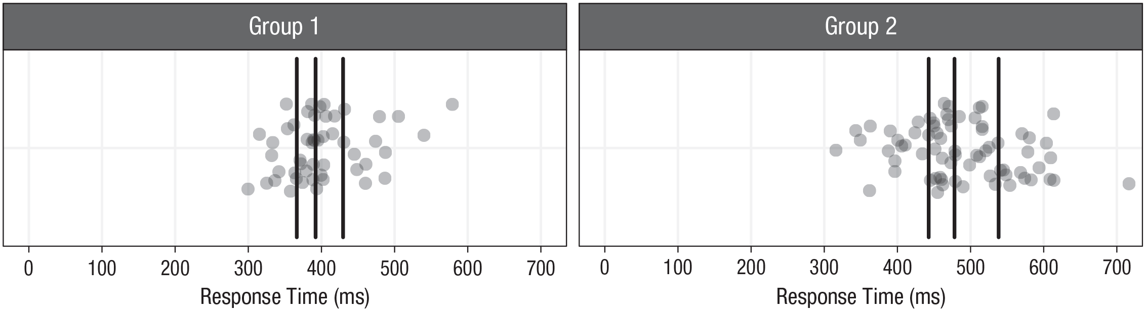
The samples from two independent groups in our example. The black vertical lines indicate the sample quartiles. Sample size is 50 in Group 1 and 70 in Group 2.

The two samples seem to differ in location and in spread: Responses tend to be slower and more spread out in Group 2 relative to Group 1. First, we make inferences about the locations using the 20% trimmed mean and the percentile bootstrap.

Difference in location

Here is the code implementing the bootstrap sampling:



nboot <- 2000 # number of bootstrap
 samples
ptrim <- 0.2 # proportion of trimming
# bootstrap sampling independently
 from each group
boot1 <- matrix(sample(g1, size =
 n1*nboot, replace = TRUE), nrow =
 nboot)
boot2 <- matrix(sample(g2, size = n2*nboot,
 replace = TRUE), nrow = nboot)
# compute trimmed mean for each group
 and bootstrap sample
boot1.tm <- apply(boot1, 1, mean,
 trim = ptrim)
boot2.tm <- apply(boot2, 1, mean,
 trim = ptrim)
# get distribution of bootstrap
 differences
boot.diff <- boot1.tm - boot2.tm

For two independent groups, bootstrap samples are generated independently from each group. This is an important principle of the bootstrap: The sampling follows the original data-acquisition process. In our example, Group 1 has a sample size of 50, whereas Group 2 has a sample size of 70. So, for each bootstrap, we sample with replacement 50 observations from Group 1 and 70 observations from Group 2, we compute the 20% trimmed mean for each group, and then we compute the difference between the groups. Figure 6 illustrates the distribution of 2,000 bootstrap differences, boot.diff, with the associated 95% confidence interval.

Fig. 6.

The bootstrap distribution of the differences between the 20% trimmed means in our example. The 95% confidence interval is depicted as an orange bar, with labels for the values of the lower (L) and upper (U) bounds.

The 95% confidence interval for the difference between the 20% trimmed means is computed like this:



alpha <- 0.05
ci <- quantile(boot.diff, probs =
 c(alpha/2, 1-alpha/2))
round(ci, digits = 1)
2.5% 97.5%
-113.7 -68.2

The confidence interval, [−114, −68], is compatible with a large range of negative values, suggesting that Population 2 is slower than Population 1. The confidence interval does not include zero, so the p value is less than .05, as computed using the code we have already presented:



null.value <- 0 # null value
pval <- mean(boot.diff < null.value) +
 mean(boot.diff == null.value)*0.5
pval <- 2*(min(pval,1-pval))
pval
[1] 0

More generally, a confidence interval can be considered an inverted hypothesis test: A 95% confidence interval, for example, contains all the hypotheses for which the p value is more than .05 (Greenland et al., 2016).

Difference in spread

We can also use the bootstrap to investigate differences in spread between the two groups. Instead of the usual standard deviation, here we use a robust estimator of variability, the median absolute deviation from the median (MAD). We can directly compute the MAD for each of the bootstrap samples we have already generated:



boot1.mad <- apply(boot1, 1, mad)
boot2.mad <- apply(boot2, 1, mad)
boot.diff <- boot1.mad - boot2.mad

The bootstrap distribution of differences between MADs is illustrated in Figure 7. We can use the same snippets of code we used previously to compute the confidence interval and the p value for the population difference, so we do not repeat them here. Given our bootstrap model, the confidence interval suggests that a large range of population differences is compatible with the data. These differences are mostly negative, which suggests that Population 2 might be more spread out than Population 1 (p = .083).

Fig. 7.

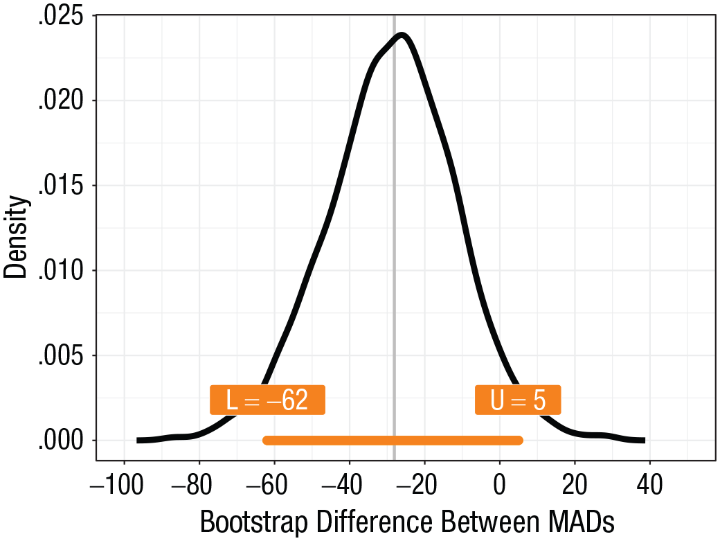
The bootstrap distribution of differences between the median absolute deviations from the median (MADs) in our example. The 95% confidence interval is depicted as an orange bar, with labels for the values of the lower (L) and upper (U) bounds.

Conclusion

This Tutorial just scratches the surface of what is possible with the bootstrap. Users might be particularly interested in applications to correlations (Pernet et al., 2013) or analysis of variance, analysis of covariance, and regression (Field & Wilcox, 2017; Wilcox, 2017). The companion R Notebook includes code to make inferences about correlation coefficients and their differences, for instance. Also, unlike the t test, the bootstrap can be combined with many robust measures of central tendency (e.g., median, trimmed means, M-estimators), and thus frees users from the tyranny of the mean. Combined with quantile estimators, the bootstrap can be used to make inferences about multiple parts of distributions and provides a far deeper understanding of how distributions differ than is possible with conventional methods (Rousselet et al., 2017). The bootstrap can also be used to estimate bias and standard errors, topics that are covered in other tutorials (Rousselet et al., 2019; Rousselet & Wilcox, 2020a).

Although the examples covered in this Tutorial may be relatively simple, the fundamental idea of sampling with replacement does scale up easily to more complex situations. Learning about sampling with replacement also means learning about simulations in an intuitive way. This knowledge can then be put to use in other contexts, for instance, to compare the behavior of different statistical methods, as we have shown. Because the bootstrap is intuitive, is easy to code, and provides an ideal stepping stone to learn about simulations, we believe, as other authors have argued, that it should be at the core of modern statistical training in psychology (Steel et al., 2019).

Moreover, a few important points about the bootstrap should be kept in mind. No matter what type of bootstrap is used, the core assumption is that the sample data can be used to approximate the shape of sampling distributions (plug-in principle); therefore, samples must be sufficiently large to provide enough information about the shape of these distributions. When sample sizes are too small, no amount of bootstrapping can lead to reliable inferences because the skewness and the tails of certain distributions cannot be captured properly. And there is no safe guideline about sample sizes: Obviously, the larger the better, and one can use simulations to assess the performance of a particular method for different sample sizes (Rousselet et al., 2019).

Among the various types of bootstrap methods, the percentile bootstrap, covered here, works well in various situations, for instance, when making inferences about trimmed means, quantiles, or correlation coefficients (Rousselet et al., 2017, 2019; Wilcox, 2017). However, percentile-bootstrap confidence intervals tend to be inaccurate in some situations because the bootstrap sampling distribution is skewed (asymmetric) and biased (consistently shifted away from the population value in one direction). To address these problems, two major alternatives to the percentile bootstrap have been suggested: the bootstrap-t and the bias-corrected and accelerated (BCa) bootstrap (Efron & Tibshirani, 1994), both of which are implemented in the boot package, for instance. However, no method dominates. For instance, whereas the bootstrap-t can lead to more accurate confidence intervals for the mean and some trimmed means than the percentile bootstrap does, a percentile bootstrap is recommended for inferences about the 20% trimmed mean (see simulation examples in Rousselet et al., 2019). And in some situations, the BCa approach can be unsatisfactory, especially for relatively small sample sizes (Good, 2005).

Because of all these options, to avoid confusion regarding reported bootstrap results, we recommend clearly stating which bootstrap method was used, in conjunction with which estimator (e.g., the percentile bootstrap with a 20% trimmed mean), and justifying these choices. We also recommend reporting the full bootstrap distribution (and the code), as it contains much more information than the confidence interval and the p value.

Finally, although the bootstrap was developed as a frequentist technique, there are interesting similarities with Bayesian statistics: Bootstrap distributions have been compared with Bayesian posterior distributions (Bååth, 2015; Rubin, 1981), and sampling with replacement from Bayesian posterior distributions is a common practice. So learning the bootstrap is also a very useful first step toward learning more advanced techniques.

Footnotes

Transparency

Action Editor: Alex O. Holcombe

Editor: Daniel J. Simons

Author Contributions

G. A. Rousselet created the figures and examples. R. R. Wilcox provided the functions implementing the bootstrap methods. C. R. Pernet verified the code. G. A. Rousselet wrote the first draft of the manuscript, and all the authors critically edited it. All the authors approved the final submitted version of the manuscript.

ORCID iD

Guillaume A. Rousselet

Notes

References

Bååth

(2015, April 18). The non-parametric bootstrap as a Bayesian model. Publishable Stuff. http://www.sumsar.net/blog/2015/04/the-non-parametric-bootstrap-as-a-bayesian-model/

Baguley

(2012). Serious stats: A guide to advanced statistics for the behavioral sciences. Palgrave Macmillan.

Baty

Delignette-Muller

M.-L.

(2015). nlstools: Tools for nonlinear regression analysis (Version 1.0-2) [Computer software]. Comprehensive R Archive Network. https://CRAN.R-project.org/package=nlstools

Baty

Ritz

Charles

Brutsche

Flandrois

J.-P.

Delignette-Muller

M.-L.

(2015). A toolbox for nonlinear regression in R: The package nlstools. Journal of Statistical Software, 66(5). https://doi.org/10.18637/jss.v066.i05

Canty

Ripley

B. D.

(2020). boot: Bootstrap functions (Version 1.3-25) [Computer software]. Comprehensive R Archive Network. https://CRAN.R-project.org/package=boot

Crawley

M. J.

(2012). The R book (2nd ed.). Wiley-Blackwell.

Dalgaard

(2008). Introductory statistics with R (2nd ed.). Springer-Verlag. https://doi.org/10.1007/978-0-387-79054-1

Davison

A. C.

Hinkley

D. V.

(1997). Bootstrap methods and their applications. Cambridge University Press. http://statwww.epfl.ch/davison/BMA/

Dienes

(2008). Understanding psychology as a science: An introduction to scientific and statistical inference. Palgrave Macmillan.

10.

Efron

(2003). Second thoughts on the bootstrap. Statistical Science, 18(2), 135–140. https://doi.org/10.1214/ss/1063994968

11.

Efron

Hastie

(2016). Computer age statistical inference. Cambridge University Press.

12.

Efron

Tibshirani

(1994). An introduction to the bootstrap. Chapman and Hall/CRC.

13.

Field

A. P.

Wilcox

R. R.

(2017). Robust statistical methods: A primer for clinical psychology and experimental psychopathology researchers. Behaviour Research and Therapy, 98, 19–38. https://doi.org/10.1016/j.brat.2017.05.013

14.

Fox

Weisberg

(2019a). car: Companion to applied regression (Version 3.0-10) [Computer software]. Comprehensive R Archive Network. https://CRAN.R-project.org/package=car

15.

Fox

Weisberg

(2019b). An R companion to applied regression (3rd ed.). Sage. https://socialsciences.mcmaster.ca/jfox/Books/Companion/

16.

Good

P. I.

(2005). Permutation, parametric, and bootstrap tests of hypotheses (3rd ed.). Springer.

17.

Greenland

Senn

S. J.

Rothman

K. J.

Carlin

J. B.

Poole

Goodman

S. N.

Altman

D. G.

(2016). Statistical tests, P values, confidence intervals, and power: A guide to misinterpretations. European Journal of Epidemiology, 31(4), 337–350. https://doi.org/10.1007/s10654-016-0149-3

18.

Grolemund

Wickham

(n.d.). R for data science. https://r4ds.had.co.nz

19.

Hesterberg

(2015a). resample: Resampling functions (Version 0.4) [Computer software]. Comprehensive R Archive Network. https://CRAN.R-project.org/package=resample

20.

Hesterberg

(2015b). What teachers should know about the bootstrap: Resampling in the undergraduate statistics curriculum. The American Statistician, 69(4), 371–386. https://doi.org/10.1080/00031305.2015.1089789

21.

Higham

D. J.

Higham

N. J.

(2016). MATLAB guide (3rd ed.). Society for Industrial and Applied Mathematics.

22.

Tumkaya

(2020). dabestr: Data analysis using bootstrap-coupled estimation (Version 0.3.0) [Computer software]. Comprehensive R Archive Network. https://CRAN.R-project.org/package=dabestr

23.

Tumkaya

Aryal

Choi

Claridge-Chang

(2019). Moving beyond P values: Data analysis with estimation graphics. Nature Methods, 16(7), 565–566. https://doi.org/10.1038/s41592-019-0470-3

24.

Limpert

Stahel

W. A.

(2017). The log-normal distribution. Significance, 14(1), 8–9. https://doi.org/10.1111/j.1740-9713.2017.00993.x

25.

Mair

Wilcox

(2020a). Robust statistical methods in R using the WRS2 package. Behavior Research Methods, 52(2), 464–488. https://doi.org/10.3758/s13428-019-01246-w

26.

Mair

Wilcox

(2020b). WRS2: A collection of robust statistical methods (Version 1.1-0) [Computer software]. Comprehensive R Archive Network. https://CRAN.R-project.org/package=WRS2

27.

Matzke

Wagenmakers

E.-J.

(2009). Psychological interpretation of the ex-Gaussian and shifted Wald parameters: A diffusion model analysis. Psychonomic Bulletin & Review, 16(5), 798–817. https://doi.org/10.3758/PBR.16.5.798

28.

Morris

T. P.

White

I. R.

Crowther

M. J.

(2019). Using simulation studies to evaluate statistical methods. Statistics in Medicine, 38(11), 2074–2102. https://doi.org/10.1002/sim.8086

29.

Peng

R. D.

(2019). simpleboot: Simple bootstrap routines (Version 1.1-7) [Computer software]. Comprehensive R Archive Network. https://CRAN.R-project.org/package=simpleboot

30.

Pernet

C. R.

Wilcox

Rousselet

G. A.

(2013). Robust correlation analyses: False positive and power validation using a new open source Matlab toolbox. Frontiers in Psychology, 3, Article 606. https://doi.org/10.3389/fpsyg.2012.00606

31.

R Core Team. (2020). R: A language and environment for statistical computing (Version 4.0.3) [Computer software]. R Foundation for Statistical Computing. https://www.R-project.org/

32.

RStudio Team. (2020). RStudio: Integrated development for R (Version 1.3.1093) [Computer software]. R Studio.

33.

Rousselet

G. A.

Pernet

C. R.

Wilcox

R. R.

(2017). Beyond differences in means: Robust graphical methods to compare two groups in neuroscience. European Journal of Neuroscience, 46(2), 1738–1748. https://doi.org/10.1111/ejn.13610

34.

Rousselet

G. A.

Pernet

C. R.

Wilcox

R. R.

(2019). A practical introduction to the bootstrap: A versatile method to make inferences by using data-driven simulations. PsyArXiv. https://doi.org/10.31234/osf.io/h8ft7

35.

Rousselet

G. A.

Wilcox

R. R.

(2020a). Reaction times and other skewed distributions: Problems with the mean and the median. Meta-Psychology, 4. https://doi.org/10.15626/MP.2019.1630

36.

Rousselet

G. A.

Wilcox

R. R.

(2020b). rogme: Robust graphical methods for group comparisons (Version 0.2.1) [Computer software]. https://github.com/GRousselet/rogme

37.

Rubin

D. B.

(1981). The Bayesian bootstrap. The Annals of Statistics, 9(1), 130–134. https://doi.org/10.1214/aos/1176345338

38.

Steel

E. A.

Liermann

Guttorp

(2019). Beyond calculations: A course in statistical thinking. The American Statistician, 73(Suppl. 1), 392–401. https://doi.org/10.1080/00031305.2018.1505657

39.

Tibshirani

Leisch

(2019). bootstrap: Functions for the book “An introduction to the bootstrap” (Version 2019.6) [Computer software]. Comprehensive R Archive Network. https://CRAN.R-project.org/package=bootstrap

40.

van Rossum

Drake

F. L.

(2009). Python 3 reference manual. CreateSpace.

41.

Wickham

(2016). ggplot2: Elegant graphics for data analysis. Springer-Verlag.

42.

Wickham

Grolemund

(2017). R for data science: Import, tidy, transform, visualize, and model data (1st ed.). O’Reilly Media.

43.

Wilcox

R. R.

(2017). Introduction to robust estimation and hypothesis testing (4th ed.). Academic Press.

44.

Wilcox

R. R.

Rousselet

G. A.

(2018). A guide to robust statistical methods in neuroscience. Current Protocols in Neuroscience, 82(1), 8.42.1–8.42.30. https://doi.org/10.1002/cpns.41

The Percentile Bootstrap: A Primer With Step-by-Step Instructions in R

Abstract

Keywords

Disclosures

Bootstrap Implementation

Bootstrap confidence interval

Bootstrap p value

Confidence interval coverage and robust estimation

Comparison of Two Independent Groups

Difference in location

Difference in spread

Conclusion

Footnotes

Transparency

ORCID iD

Notes

References