Sage Journals: Discover world-class research

Abstract

Frequently, researchers in psychology are faced with the challenge of narrowing down a large set of predictors to a smaller subset. There are a variety of ways to do this, but commonly it is done by choosing predictors with the strongest bivariate correlations with the outcome. However, when predictors are correlated, bivariate relationships may not translate into multivariate relationships. Further, any attempts to control for multiple testing are likely to result in extremely low power. Here we introduce a Bayesian variable-selection procedure frequently used in other disciplines, stochastic search variable selection (SSVS). We apply this technique to choosing the best set of predictors of the perceived unpleasantness of an experimental pain stimulus from among a large group of sociocultural, psychological, and neurobiological (functional MRI) individual-difference measures. Using SSVS provides information about which variables predict the outcome, controlling for uncertainty in the other variables of the model. This approach yields new, useful information to guide the choice of relevant predictors. We have provided Web-based open-source software for performing SSVS and visualizing the results.

Keywords

neuroscience Bayesian modeling uncertainty multiple regression reproducibility stochastic search variable selection open data open materials

Consider a challenge many researchers face in different contexts: Given a set of candidate predictors, how should one decide which smaller set of predictors to include in a regression model? Ideally, the set of relevant predictors would be based on strong theory, the size of the sample would be generous, and the number of candidate predictors would be tiny in comparison with the sample size. In this ideal case, it may be simple to include all relevant predictors and report the results.

However, as the pool of potentially relevant predictors grows, the problem becomes thornier. Perhaps theory predicts that any of the predictors might be related to the outcome, or perhaps there is insufficient prior research to guide the choice. If all predictors are included at once, very few may be meaningfully related to the outcome while simultaneously competing for variance with all the others. In the extreme case, if the number of candidate predictors meets or even exceeds the sample size, including all the predictors is not possible. Alternatively, often the bivariate correlations between each predictor and the outcome are screened, and predictors with significant correlations are included in a multivariate model (e.g., Lavie et al., 1995; Safren et al., 2016; Schultz et al., 2004). This common practice has substantial weaknesses, however. When predictors are correlated, as they very often are in psychology, screening predictors on the basis of bivariate correlations may easily translate into a multivariate model in which no predictors have a meaningful, unique relationship with the outcome (i.e., partial regression coefficients are nonsignificant). Other relationships may not be detected without controlling for one or more confounding variables. Further, if any effort is made to guard against false positives by controlling for multiple testing, power to detect meaningful effects is greatly reduced.

In contrast, it may be appealing to take an algorithmic approach to selecting predictors, such as stepwise regression or all-possible-subsets regression. In stepwise regression, a model is built by automatically adding and removing individual predictors, one step at a time, on the basis of the significance of individual terms or changes in R². This produces results that capitalize highly on sampling error, have poor replicability, and do not correctly identify the best predictor set of a given size (e.g., Henderson & Denison, 1989; Thompson, 1995). Even though the use of stepwise regression has long been discouraged, it continues to be used (McNeish, 2015), perhaps in part because the method is an easily implemented solution to a vexing problem. All-possible-subsets regression is based on selecting a model with the best R² or other criterion, such as Akaike’s information criterion or the Bayesian information criterion. Because the number of possible models increases exponentially with the number of predictors (e.g., 30 predictors means 2³⁰, or 1,073,741,824, possible models), methods to select the “best” model on the basis of all possible subsets are also highly sensitive to chance variability and have poor generalizability (Olejnik, Mills, & Keselman, 2000).

In this article, we present stochastic search variable selection (SSVS), a Bayesian variable-selection method to aid researchers facing this common scenario. The article is accompanied by an online application for performing SSVS and visualizing the results. The approach we demonstrate is not new (George & McCulloch, 1993, 1997), but to our knowledge, it has rarely been applied in psychological research. SSVS¹ is a popular method in more biologically based research, such as genomewide association studies (Lee, Sha, Dougherty, Vannucci, & Mallick, 2003), but has also been used in applications ranging from health outcomes (e.g., range of predictors for metabolic syndrome; Cheraghi et al., 2018) to economic variables (e.g., economic and social factors associated with inflation; Sala-I-Martin, Doppelhofer, & Miller, 2004). By accounting for model uncertainty, Bayesian variable-selection methods both increase power and decrease false-positive results, compared with traditional approaches (Swartz, Yu, & Shete, 2008; Viallefont, Raftery, & Richardson, 2001). SSVS provides information about the relative importance of predictors,² accounting for uncertainty in which other predictors are included in the model. In this article, we present a common formulation of SSVS and compare it with standard approaches in the context of an example from our own work in which we faced the variable-selection problem. Many other forms of Bayesian variable selection exist, and we hope that this article will help spark interest in understanding which formulations perform best under which conditions (we recommend Fragoso, Bertoli, & Louzada, 2018, for a recent systematic review).

First, we introduce our focal example and describe SSVS. We then compare results obtained with SSVS and with standard variable selection based on bivariate relationships and introduce our online application for performing SSVS. Finally, we place SSVS in context with other variable-selection methods and present results of a simulation comparing SSVS with lasso regression (Tibshirani, 1996).

Disclosures

The scripts and documentation for the simulation, plots, and applied analyses in this article are available online at the Open Science Framework, at https://osf.io/m8djx/. The Supplemental Material (http://journals.sagepub.com/doi/suppl/10.1177/2515245919885617) contains descriptions of and descriptive statistics for all the questionnaires used in the reported analysis.

The Example: Predicting the Perceived Unpleasantness of Pain

Although pain is a universal part of (neurotypical) human experience, the way people experience and respond to pain is highly variable. Individual differences in pain sensitivity likely originate from a variety of sources, as we have outlined in our recently published neurocultural model of pain (S. R. Anderson & Losin, 2017). These sources range from genetic variation related to the endogenous pain modulatory system, to socially learned coping styles, to previous experiences with pain and other stressful life events. Characterizing the contributions that these different psychological, sociocultural, and neurobiological factors make to individual differences in pain is of great interest to both basic scientists and clinicians. Yet, because of the myriad of potential factors contributing to individual differences in pain, the combination of factors that are most influential is still not well understood. SSVS is therefore an ideal approach for tackling this problem.

Here we apply SSVS to a data set from an experiment in which participants underwent experimental pain induction using contact heat to the forearm while undergoing functional MRI (fMRI). During the pain stimulation, we collected several brain-activity measures, and after each heat stimulation, participants rated the intensity and unpleasantness of the pain they experienced. For the present analysis, we focus on the unpleasantness ratings as our dependent variable. These ratings were averaged over nine trials (α = .91).

Prior to their lab visit, participants completed a battery of self-report questionnaires online via Qualtrics, and additional self-report measures were administered during the fMRI scanning session. The measures selected were hypothesized to contribute to individual differences in pain rating and to assess different aspects of cultural background and the pain experience outlined in our neurocultural model of pain, including stressful life experiences, mood, beliefs about the causes and consequences of pain, responses to pain (e.g., coping strategies), and pain context (e.g., trust in the person performing the painful procedure). We also included measures of personality and demographics, as those have also been demonstrated to influence pain responses (K. O. Anderson, Green, & Payne, 2009; Kim et al., 2017; Shiomi, 1978). The self-report measures corresponding to each category are listed in Table 1. Details and descriptive statistics for each questionnaire are available in the Supplemental Material.

Table 1.

Self-Report Questionnaires Administered Prior to the Experimental Pain Induction

Predictor category	Measures
Pain precursors: stressful life events	Alcohol, Smoking, and Substance Involvement Screening Test (ASSIST) Barratt Simplified Measure of Social Status (BSMSS) Brief History of Pain Questionnaire (BHPQ, 3 subscales) Experiences of Discrimination (EOD, 5 subscales) Life Events Checklist (LEC) Stress and Adversity Inventory (STRAIN, 6 subscales) Williams Major and Everyday Discrimination Questions (WQ)
Pain precursors: mood	Five Facet Mindfulness Questionnaire (FFMQ, 2 subscales) Imaginal Process Inventory (IPI, 3 subscales) Mood and Anxiety Symptom Questionnaire (MASQ) Positive and Negative Affect Schedule (PANAS, 4 subscales) Ruminative Response Scale (RRS, 3 subscales) State and Trait Anxiety Inventory form X (STAI)
Pain precursors: beliefs and expectations	Fear of Pain Questionnaire-III (FPQ, 3 subscales) Health and Illness Scale (HIS, 7 subscales) Pain Beliefs Questionnaire (PBQ, 2 subscales)
Pain responses	Coping Strategies Questionnaire 24 (CSQ, 8 subscales) Emotion Regulation Questionnaire (ERQ, 2 subscales) Kohn Reactivity Scale (KRS) Pain Catastrophizing Scale (PCS, 3 subscales)
Pain context and communication	Similarity Visual Analog Scale (SVAS, 2 subscales) Trust Visual Analog Scale (TVAS) Wake Forest Physician Trust Scale (WFPTS)
Personality and identity	Big Five Inventory (BFI, 5 subscales) Multigroup Ethnic Identity Measure (MEIM)
Demographic variables	Items asking participants to report their age, sex, and race-ethnicity

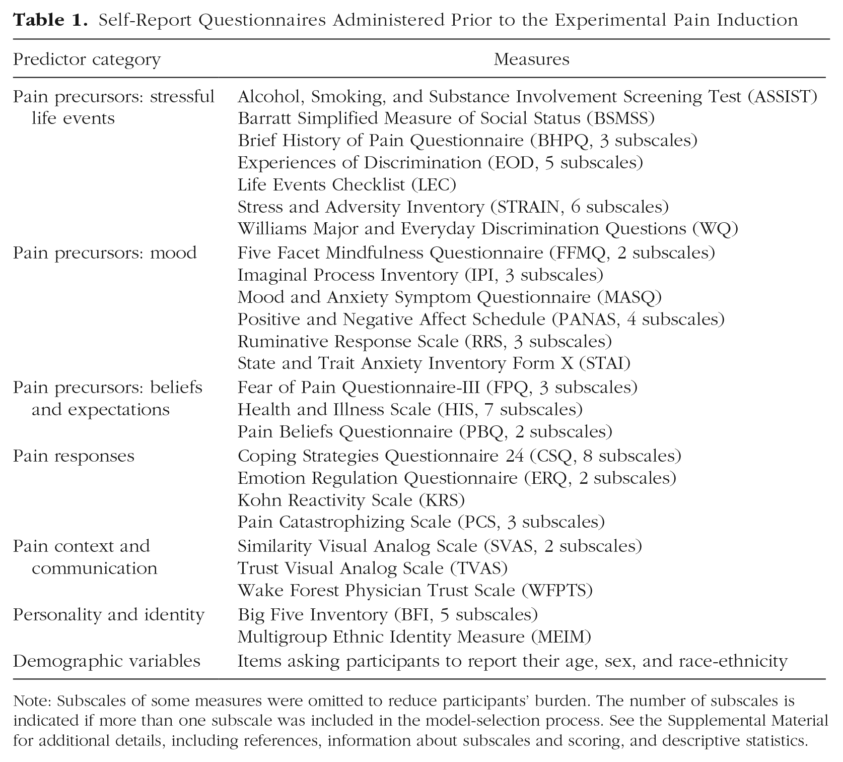
Note: Subscales of some measures were omitted to reduce participants’ burden. The number of subscales is indicated if more than one subscale was included in the model-selection process. See the Supplemental Material for additional details, including references, information about subscales and scoring, and descriptive statistics.

Finally, we included in our analysis three measures of brain responses to pain. The first brain measure was each person’s expression of the Neurologic Pain Signature (NPS), a machine-learning-derived multivariate pain-predictive pattern of brain activity (Wager et al., 2013). The second and third measures focused on activity within the nucleus accumbens (NAcc) and the ventromedial prefrontal cortex (vmPFC). These two brain regions lie outside the regions involved in the NPS but are associated with the affective-motivational aspects of pain(Baliki et al., 2012) and thus may be of particular relevance to predicting pain unpleasantness (Price, 2000). The Supplemental Material provides a full description of each brain measure.

As does standard regression analysis, SSVS requires complete data for the dependent variable and all predictors. However, whereas a series of regression models can maximize available sample size on a model-by-model basis (i.e., through pairwise deletion), SSVS requires complete cases for all measures included in the analysis. In the initial pool of 104 predictors for 93 participants, the rates of missingness were low for all the predictors (mean missingness = 2%), but only 48 participants had complete data on all predictors. Therefore, in order to maximize both sample size and the candidate predictor set for this analysis, we excluded predictors with more than 6% missing responses and retained cases with complete data for the remaining measures. Our final data set for this example consisted of data from 74 participants who provided values for our dependent variable, pain unpleasantness ratings, and 75 predictors of those ratings.

Note that although in this example we had about as many variables as observations, SSVS is applicable to less extreme scenarios (e.g., 10 candidate predictors in a large sample) or more extreme scenarios. In fact, SSVS has been regularly applied in genomewide association studies involving thousands of genes (Fridley, 2009; Lee et al., 2003), though some computational adjustments may be necessary when the number of predictors far exceeds the sample size. Other useful applications different from the example discussed here might be to determine a subset of predictors that predict a behavior or diagnosis. For example, which set of predictors together best predict a measure of inflammation, which individuals evacuate ahead of a hurricane, or willingness to get HIV testing?

The Standard Approach

First we consider the results obtained for our example when we selected predictors on the basis of bivariate correlations with the pain unpleasantness ratings. In such an analysis, researchers might choose to consider predictors with correlations that are significant at the α = .05 level, or they might choose a more liberal cutoff, such as α = .1, to prioritize discovery. A more stringent cutoff or adjustment might be adopted to account for multiple comparisons. In this example, the p values for the bivariate relationships with unpleasantness ratings were less than .1 for 10 predictors, less than .05 for 8 predictors, and less than .01 for 3 predictors. A Benjamini-Hochberg correction for multiple comparisons would result in 1 significant predictor. The choice of cutoff is arbitrary, but in our experience researchers tend to use a less stringent cutoff than α = .05 for the purpose of exploratory variable selection, so we adopted this approach for our example.

Table 2 shows the results of a regression model including the 10 predictors with a bivariate correlation meeting the criterion of α = .10. In the full model, 3 predictors remained significant: not having filed a formal complaint of discrimination (Experiences of Discrimination Subscale 5), pain catastrophizing during the fMRI scan (Coping Strategies Questionnaire Subscale 5), and belief in supernatural causes of illness (Health and Illness Scale Subscale 7). The model R² indicates that together the set of predictors explained 45.9% of the variance in pain ratings.

Table 2.

Regression Results Predicting Ratings of Unpleasantness

Predictor	r	Coefficient (b) in the bivariate selection model (R² = .459, adjusted R² = .373)	MIP	Coefficient (b) in the SSVS model (R² = .593, adjusted R² = .529)
Stressful events
Less worry about discrimination (EOD3)	.24*	0.41 [−1.46, 2.28]	.74	−1.08 [−3.04, 0.88]
Higher global perceived discrimination (EOD4)	.03		.86	−2.91* [−5.22, −0.61]
Has not filed a discrimination complaint (EOD5)	.36*	−13.60* [−24.36, −2.85]	.84	−15.25* [−24.66, −5.83]
Mood
Daydreaming frequency (IPI2)	.21	0.11 [−0.14, 0.36]	.35
Pain beliefs
Fear of minor pain (FPQ1)	.05		.72	−0.42 [−0.87, 0.03]
Fear of medical pain (FPQ3)	.23*	0.10 [−0.34, 0.54]	.65
Belief that exposure causes illness (HIS3)	.11		.93	2.55* [0.88, 4.21]
Belief in supernatural causes of illness (HIS7)	.21	2.55* [0.24, 4.87]	.85	2.68* [0.61, 4.75]
Pain responses
Pain catastrophizing during the scan (CSQ5)	.44*	0.72* [0.21, 1.23]	.99	1.08* [0.71, 1.44]
Cognitive coping during the scan (CSQ8)	−.31*	−0.37 [−0.82, 0.09]	.57
Pain context
Trust in experimenter (TVAS)	−.24*	−0.03 [−0.21, 0.15]	.47
Brain responses
Mean vmPFC activity	−.15		.67	−5.13* [−8.90, −1.36]
Demographics
Hispanic	−.28*	−5.48 [−12.06, 1.11]	.74	−5.48 [−11.04, 0.07]
Black	.28*	−0.53 [−9.15, 8.10]	.68	5.21 [−1.98, 12.40]

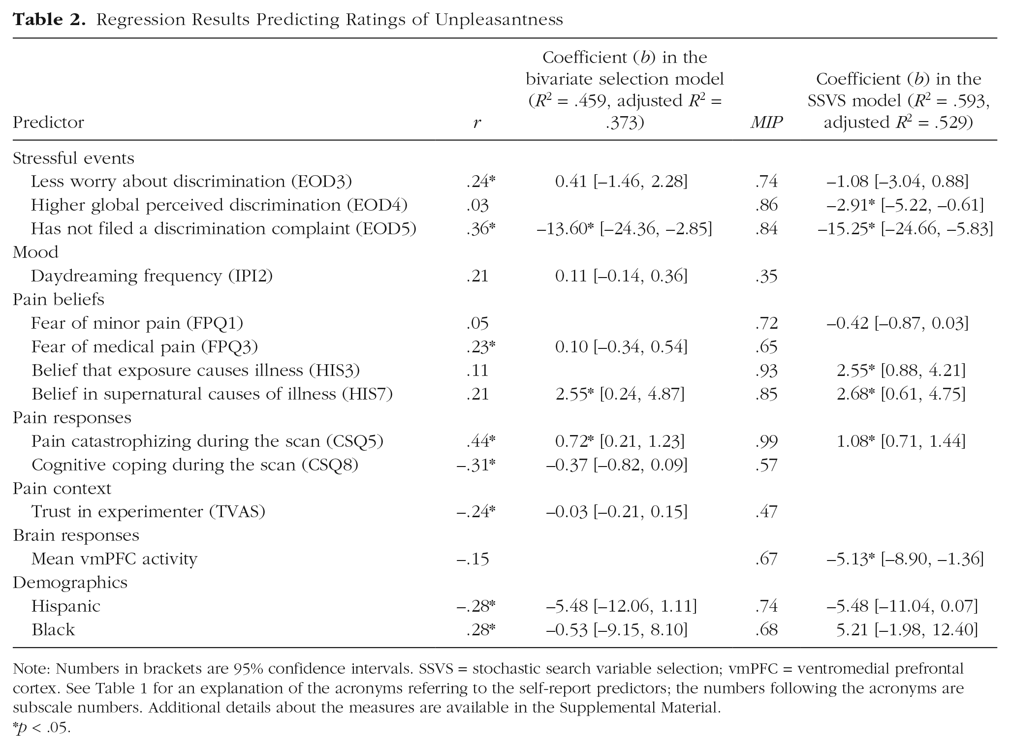
Note: Numbers in brackets are 95% confidence intervals. SSVS = stochastic search variable selection; vmPFC = ventromedial prefrontal cortex. See Table 1 for an explanation of the acronyms referring to the self-report predictors; the numbers following the acronyms are subscale numbers. Additional details about the measures are available in the Supplemental Material.

p < .05.

Fundamentally, each individual correlation coefficient tests a bivariate relationship, providing a response to the question, “Is there a significant relationship between a given predictor x and outcome y, ignoring all other factors?” The multivariate regression model then provides, for each predictor, a response to the question, “Is there a significant relationship between x and y, above and beyond the relationships for all the other predictors in the model?” Unfortunately, the bivariate tests may select a set of predictors that are all themselves highly intercorrelated, and they may be redundant in a model together. Or a predictor may be meaningfully related to the outcome only when the model controls for one or more other predictors. By contrast, SSVS can be used to answer a slightly different question: “Is a given x a consistent predictor of y, accounting for uncertainty in the other variables included in the model?”

Stochastic Search Variable Selection

Briefly, SSVS samples thousands of regression models in order to characterize the model uncertainty regarding both the predictor set and the regression parameters. The models are selected using a sampling process that is designed to select among “good” models, that is, models with high probability. After sampling, rather than selecting the best model according to a specified criterion (e.g., the best Akaike’s or Bayesian information criterion or the highest model R²), researchers can examine the proportion of times each predictor was selected, which provides information about which predictors reliably predict the outcome, accounting for uncertainty in the other predictors in the model.

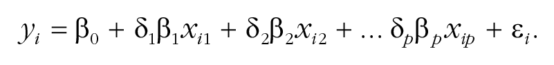
The SSVS procedure builds upon a standard regression model for y with some number of predictors p:

y_{i} = β_{0} + β_{1} x_{i 1} + β_{2} x_{i 2} + . . . β_{p} x_{i p} + ε_{i} .

In SSVS, parameter estimates are obtained using a Bayesian framework for estimation, rather than the method of ordinary least squares. In the Bayesian framework, in addition to the regression model for the data, a prior distribution is specified for each parameter. Prior distributions are simply expressions of the researcher’s beliefs (and uncertainty) about the values of the parameters. Bayesian estimation combines these priors with the model and data to arrive at the posterior distribution, which summarizes updated beliefs and uncertainty about the parameters.

A researcher could choose to provide no prior information about the intercept by specifying a totally flat prior for it (e.g., Uniform(–∝,∝)), as we did for our focal example. For each regression coefficient, the prior might be normally distributed, be centered at zero, and have large variance. For example, N(mean = 0, SD = 10) would indicate a belief that zero is the most likely value of the coefficient and that most values are less than 20 in absolute value. Because the model is more easily estimated in terms of the inverse residual variance, or precision (1/σ²), a prior for this parameter could be $~ G a m m a (a = . 01, b = . 01)$ , which would allow positive values in a wide range. This is the prior specification we used for the analysis presented later in this section.

Simply adding prior distributions to a regression model to make it Bayesian does not actually help solve the variable-selection problem, however. The results from Bayesian estimation of the model as just specified would be essentially identical with the results from ordinary least squares regression (given that the priors are relatively uninformative). Although this model could be used to get an estimate for every β, SSVS is useful when the researcher believes (as we did) that many of the βs are essentially zero and wants to screen out candidate predictors that are not important.

Therefore, the final component of the model is a set of binary indicator variables δ_j, one for each predictor, that toggle predictors in and out of the model:

y_{i} = β_{0} + δ_{1} β_{1} x_{i 1} + δ_{2} β_{2} x_{i 2} + . . . δ_{p} β_{p} x_{i p} + ε_{i} .

If δ_j = 1, variable j is included in the model. If δ_j = 0, variable j is not included (and its β_j is not estimated). SSVS (George & McCulloch, 1993) treats the full set of indicator variables δ as unknown parameters to be estimated. The estimation is designed to characterize the uncertainty about the most probable values for the coefficients β and the best set of predictors δ.

The model specification also includes a prior probability for each δ_j; we chose the common value of .5, so that each predictor had a 50/50 prior probability of being included the model. The resulting prior for the regression coefficients in SSVS is called a spike-and-slab prior, pictured in Figure 1, because this distribution is a mixture of a spike at zero and a relatively flat “slab” of nonzero values.

Fig. 1.

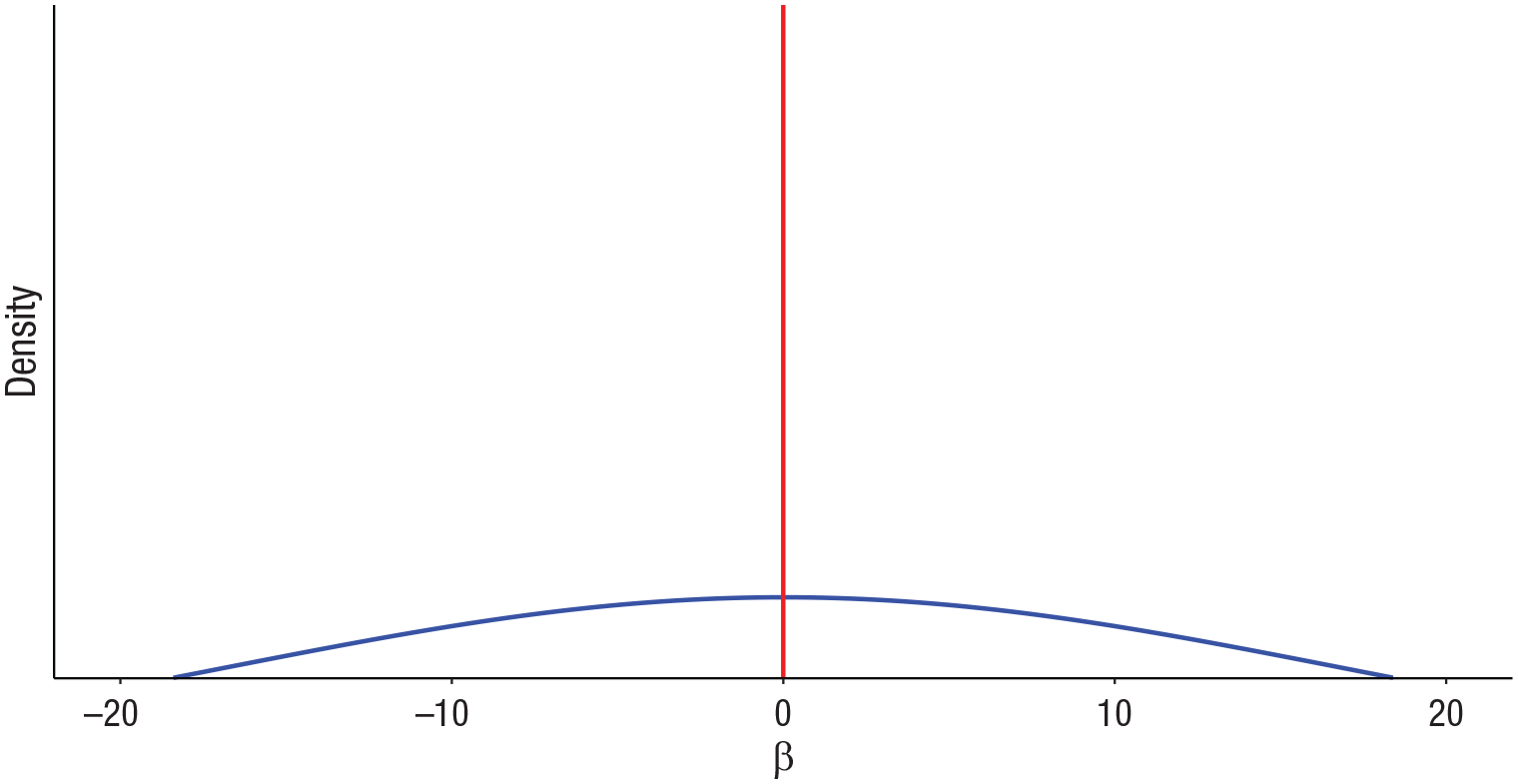
Illustration of a spike-and-slab-mixture prior distribution for regression coefficients.

The model parameters are estimated using Markov chain Monte Carlo (MCMC) estimation, which is a method used in Bayesian statistics to obtain samples from the posterior distribution. These samples characterize the uncertainty about probable values for the parameters, indicating which predictors should be retained in the model and their associated regression coefficients.

For our example of predicting pain unpleasantness ratings, we ran the MCMC sampler for 10,000 iterations. Because MCMC requires a burn-in period to help ensure that the chain converges to the target distribution, we discarded the first 1,000 samples. Note that it is important to standardize the explanatory variables before performing variable selection, so that the priors (which have a fixed scale) do not differentially influence predictors that are on different scales. After performing SSVS, it is fine to use whatever scale is easiest for interpretation. At each iteration, estimates of inclusion indicators, regression coefficients, and (inverse) variance are obtained. Figure 2 shows the estimates of the regression coefficients for each of the 75 predictors in a single iteration of the sampler. The predictors with a coefficient value of zero are those that were not included in the model for this particular iteration (i.e., δ_j = 0 for these predictors).

Fig. 2.

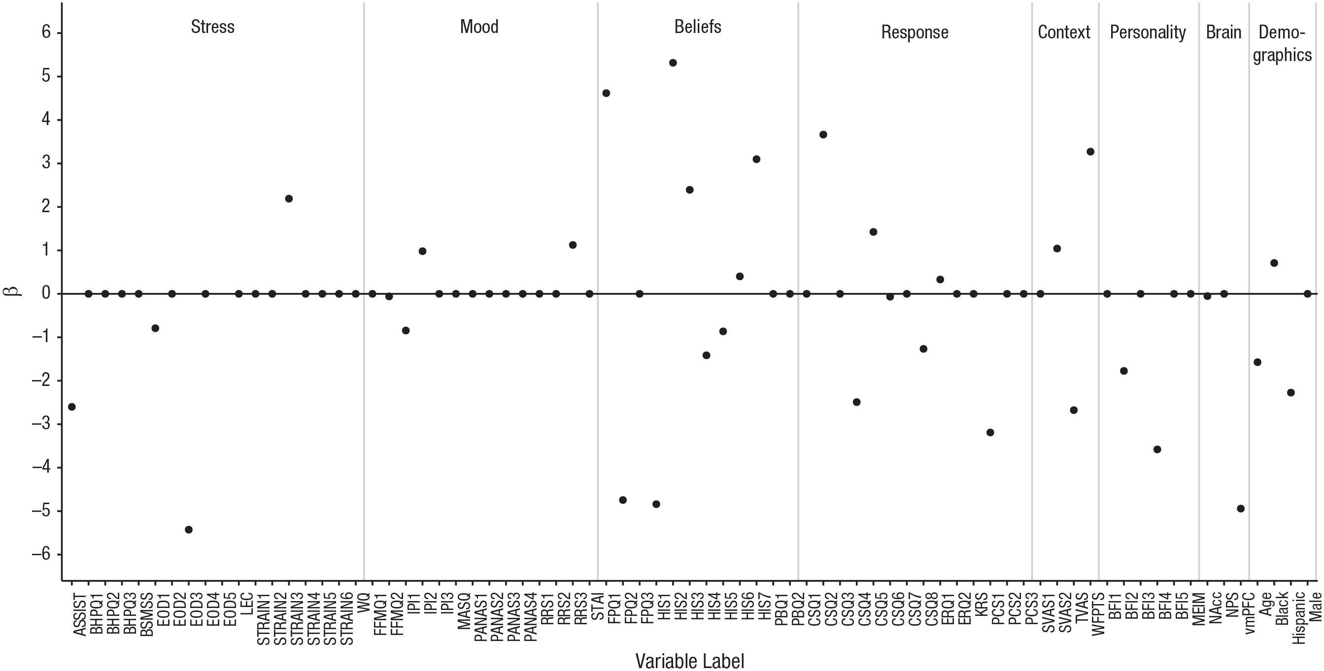
Results for the focal example: estimated beta coefficients from Iteration 7,000 of the sampler. Coefficients of zero indicate predictors not selected into the model in this iteration. See Table 1 for an explanation of the acronyms for the self-report variables; the numerical suffixes indicate subscales of these measures. Neurobiological measures taken during the pain induction were activity in the nucleus accumbens (NAcc), expression of the Neurological Pain Signature (NPS), and activity in the ventromedial prefrontal cortex (vmPFC). See the Supplemental Material for full details on the measures.

In 10,000 iterations of the sampler, only a tiny fraction of the possible models would be visited; we could not hope to visit all models and choose the single best one. Fortunately, our goal was to sample many high-probability models and identify the predictors that appeared most often. The relevant information is summarized in Figure 3, which shows the proportion of times each predictor was included in the sampled models, referred to as the marginal inclusion probability (MIP). It is interesting to compare the inclusion probability for each predictor with the magnitude of its correlation with pain unpleasantness, also plotted in Figure 3. Although higher correlations tend to correspond to higher inclusion probabilities, the relationship between bivariate correlation and MIP is imperfect, r(73) = .54, p < .001.

Fig. 3.

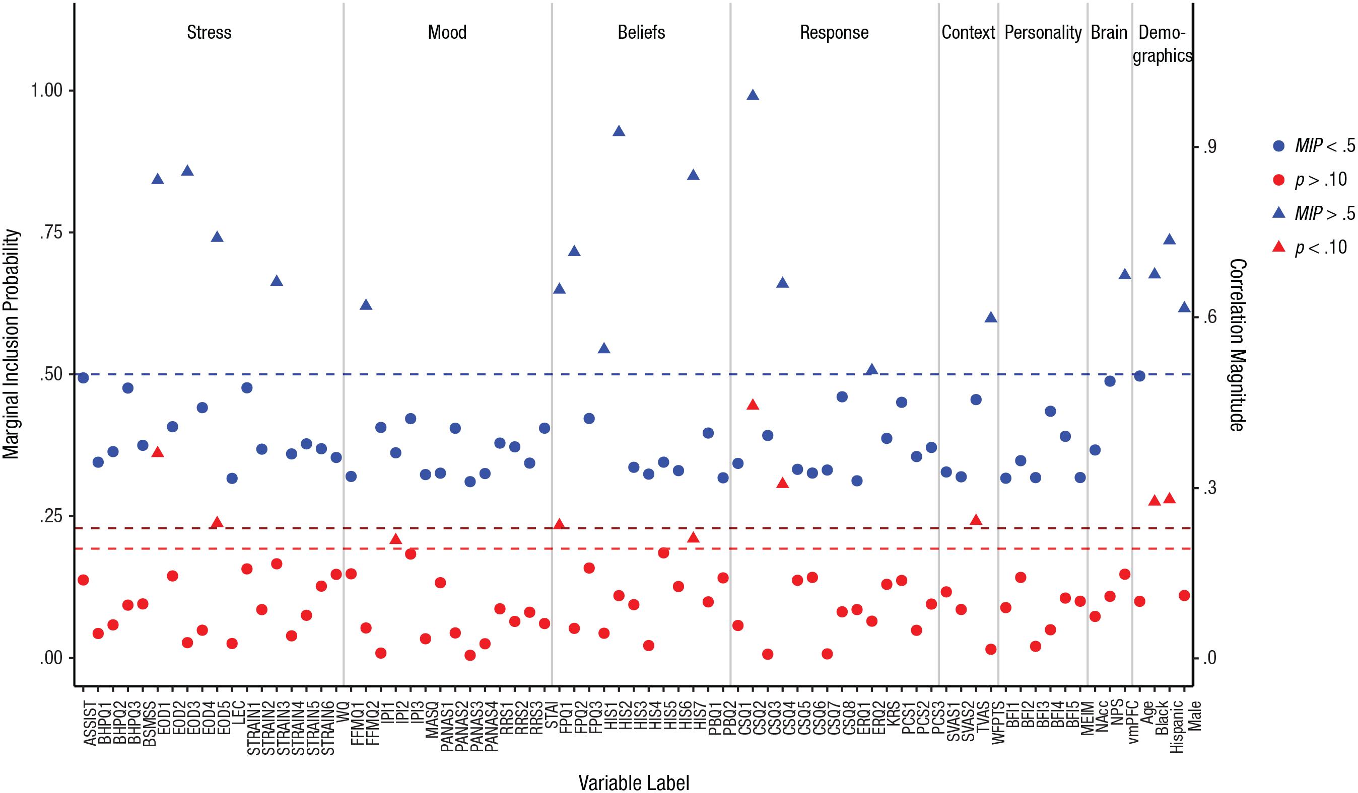
Results for the focal example. Marginal inclusion probabilities (MIPs) after stochastic search variable selection (prior inclusion probability = .5) are shown in blue. The predictors’ correlations with pain unpleasantness are shown in red. Triangles indicate variables selected by each method (i.e., MIP > .5, correlation p < .10, two-tailed). See Table 1 for an explanation of the acronyms for the self-report variables; the numerical suffixes indicate subscales of these measures. Neurobiological measures taken during the pain induction were activity in the nucleus accumbens (NAcc), expression of the Neurological Pain Signature (NPS), and activity in the ventromedial prefrontal cortex (vmPFC). See the Supplemental Material for full details on the measures.

To assess MCMC convergence and ensure that SSVS results are stable, it is necessary to compare results across two or more chains using random starting values (Swartz et al., 2013). Unstable results across chains would suggest that more iterations are needed for MCMC convergence and that the number of burn-in iterations should be increased. We ran SSVS a second time and computed the correlation between the estimated MIPs for each parameter across the two chains. The correlation we obtained was above .99.

In this example, we found 20 predictors with MIPs of .5 or greater. Although we could have chosen to include all of these predictors in a model together, .5 is not a firm cutoff or recommended threshold, and 20 predictors is still too large a set for meaningful interpretation. Visualizing the inclusion probabilities as in Figure 3 makes it possible to examine the pattern of relative magnitudes. A major reason why researchers should not rely on a specific cutoff for the MIPs is that they will vary depending on the sample size, the total number of predictors, and the prior probability of inclusion; however, the pattern of relative MIPs (i.e., which predictors have the highest MIPs) should remain substantially stable (see Box 1). Our choice of .5 as the prior inclusion probability may seem reasonably “uninformative” (or objective); however, note that this value actually implied prior belief that the model should include .5 × 75, or 37.5, predictors, which was still too large for our sample size.

Box 1.

The Effect of the Prior Inclusion Probability

We selected .5 as the prior probability of inclusion for each predictor, but how much did this value affect the predictors’ marginal inclusion probabilities (MIPs), the values we obtained from the posterior? Figure 4 shows the MIPs obtained for a range of prior inclusion probabilities, from .1 to .9 (the prior probability was equal for all predictors).

Fig. 4.

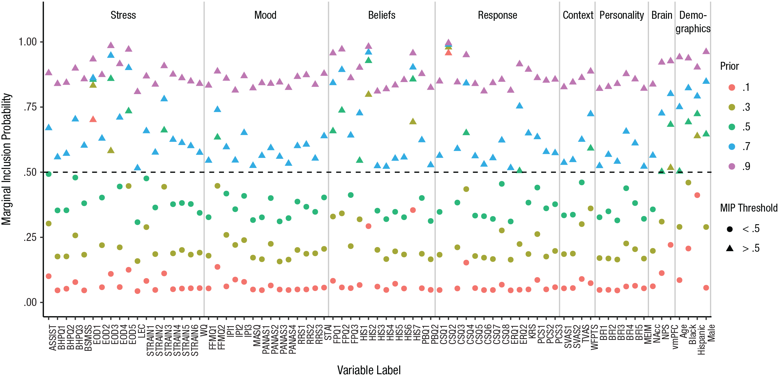
Results for the focal example: marginal inclusion probabilities (MIPs) for each variable after stochastic search variable selection for a range of prior inclusion probabilities (.1–.9). A triangle indicates that the variable met the threshold for selection (i.e., MIP > .5). See Table 1 for an explanation of the acronyms for the self-report variables; the numerical suffixes indicate subscales of these measures. Neurobiological measures taken during the pain induction were activity in the nucleus accumbens (NAcc), expression of the Neurological Pain Signature (NPS), and activity in the ventromedial prefrontal cortex (vmPFC). See the Supplemental Material for full details on the measures.

There was a clear effect of the prior probability on the MIPs. However, the relative pattern across predictors was stable. For example, the predictors with the 10 largest MIPs were the same whether the prior probability was .3 or .5. Choosing more extreme prior values, especially .9, resulted in less clear separation in MIPs among predictors with moderate values. In general, selection of a reasonable prior probability (given the sample size and number of predictors) has some effect on the magnitude of the MIPs, but does not have a strong influence on which predictors have the highest MIPs.

For our example, we chose to select the predictors with the 10 highest MIPS, which also gave us a model with the same number of predictors as the model based on bivariate correlations. Table 2 shows the results of a standard regression model in which we included the 10 predictors with the highest MIPs. This subset of 10 predictors chosen using SSVS has some overlap with the predictor set chosen via the bivariate selection model: Six predictors were chosen using both model-building strategies. However, note that 6 of the 10 predictors in the SSVS selection model significantly predicted unpleasantness ratings, whereas the bivariate selection resulted in 3 significant predictors. The 3 significant predictors in the SSVS model that were not included in the bivariate selection model are belief that exposure causes illness (Health and Illness Scale Subscale 3), mean activity in the vmPFC during pain, and global perceptions of racial discrimination (Experiences of Discrimination Subscale 4). This model has an R² value of .59 (adjusted R² = .53) and explains 13% more of the variability in pain unpleasantness ratings compared with the alternate model with the same number of predictors.

Online Application for SSVS

One barrier to the use of SSVS analyses in psychological research has been the lack of an easy-to-use tool with which to conduct such analyses. Some R packages, such as BoomSpikeSlab (Scott, 2018), offer functionality for SSVS analyses. However, these packages can be confusing and difficult to implement, and some require extensive R coding experience. All of these factors may discourage researchers from using these packages. To address this barrier, we used the shiny package (Chang, Cheng, Allaire, Xie, & McPherson, 2018) in R (R Core Team, 2017) to create a free Web application called SSVSforPsych (https://ssvsforpsych.shinyapps.io/ssvsforpsych/). This user-friendly Web application is outfit-ted with a graphical user interface that relieves the need for complicated coding. The application code builds on R code for SSVS (Reich, 2014). We hope that SSVSforPsych will enable even users who are unfamiliar with R to easily perform variable selection and visualize the results.

After navigating to the SSVSforPsych Web page, users can upload their data in a variety of common file formats (e.g., comma-delimited, text, Excel, SPSS). If predictors are unstandardized, the program will perform standardization. Users then have the option to toggle the parameter values of several inputs in the SSVS analysis, including the prior inclusion probability, the number of burn-in iterations, and the number of samples. The application defaults to a prior inclusion probability of .5, 10,000 samples, and 1,000 burn-in (discarded) iterations. After selecting parameter values, users select the set of predictors and the outcome they wish to analyze. Additionally, they have the option to select random starting values, which should be used when assessing MCMC convergence, as discussed in the previous section.

After the sampling concludes, SSVSforPsych uses the ggplot2 graphics package (Wickham, 2016) to generate a table of the results and a plot (similar to Fig. 3) displaying the MIPs. Tables and plots can be downloaded as .csv spreadsheets and .png plots. SSVSforPsych automatically updates results, tables, and graphs in real time when users submit changes to any of the inputs, so users can analyze their data under various statistical assumptions. For example, if the prior probability is changed from .5 to .3, SSVSforPsych will rerun the analysis to reflect the new estimated values.

SSVSforPsych is not designed to handle missing data, and attempts to run analyses with missing predictor or outcome data may result in error messages or misleading results. We advise users to upload data without missing values for any variables to be used in the analysis. However, developing software for performing SSVS in the presence of missing data is an important direction for future research.

Comparison With Other Methods

Many other approaches to reducing a candidate set of predictors exist. These include ridge regression, the lasso (Tibshirani, 1996), the elastic-net lasso (Zou & Hastie, 2005), various machine-learning approaches (see, e.g., Hastie, Tibshirani, & Friedman, 2009), and principal components analysis. In general, machine-learning approaches focus on prediction rather than interpretation of the predictor set. Similarly, principal components analysis performs data reduction, but interpretation of the components as predictors is not appropriate. Dominance analysis (Budescu, 1993) is another method used to evaluate the relative importance of predictors within a regression model; it is used to rank a set of predictors within a defined model and not for variable selection. Lasso methods are most similar to SSVS, in that they can be used to make binary decisions about inclusion or exclusion of predictors. In fact, a connection between lasso methods and some SSVS formulations has recently been demonstrated under some conditions (Yuan & Lin, 2005). However, whereas SSVS provides continuous information about each predictor variable’s importance, the lasso provides only binary decisions about inclusion. The continuous information provided by SSVS is helpful because, as we did in our example, researchers may decide to balance parsimony with prediction.

Whereas ordinary least squares regression simply minimizes the sum of squared residuals (SS), the lasso adds an additional term (the sum of the absolute values of all coefficients), which penalizes coefficients to avoid overfitting, with the result that some coefficients are set to zero:

l a s s o = S S + λ \sum_{j = 1}^{p} β_{j} .

The parameter λ controls the strength of the penalty, and typically an algorithm is used to obtain the λ value that minimizes cross-validation error. Applying this penalty is called regularization, a topic we expand on in Box 2. Researchers have shown that SSVS outperforms lasso techniques in certain conditions, especially when many predictors are being investigated and when the number of predictors is larger than the sample size, such as in genomewide association studies (Guan & Stephens, 2011; Srivastava & Chen, 2009).

Box 2.

Two Goals: Regularization and Variable Selection

There is a very important distinction between lasso regression and stochastic search variable selection (SSVS) as we present them here: In lasso regression, regularization (which shrinks coefficients) is usually performed in the same step as variable selection. Variable selection and regularization can also be performed in a single step in SSVS, by examining the distribution of estimates over all Markov chain Monte Carlo samples (including any iterations in which βj = 0). Combining regularization with variable selection has the effect of minimizing out-ofsample prediction error. Because our goal was to demonstrate the use of variable selection to narrow down a set of predictors derived from theory, we chose to perform variable selection and estimation in separate steps: Specifically, variable selection was followed by ordinary least squares estimation to obtain model estimates. Therefore, our estimates were not regularized. This two-stage approach is common for applications of SSVS (e.g., Swartz, Kimmel, Mueller, & Amos, 2006; Swartz et al., 2013), and it can also be used for lasso regression, in which case it is referred to as postlasso estimation (Belloni & Chernozhukov, 2013; Efron, Hastie, Johnstone, & Tibshirani, 2004).

However, because the literature comparing Bayesian estimation with the lasso is sparse and disjointed, and to better demonstrate a comparison of SSVS with the lasso, here we summarize results of a simulation study, based on our focal example, in which we varied sample size (N = 75, N = 150) and the reliability of the outcome (perfect: α = 1; moderate: α = .8; low: α = .5). For each of the six conditions, we simulated 500 data sets, using the covariance matrix from our example as the population generating model; correlations between the predictors and outcome were adjusted to account for attenuated or disattenuated relationships depending on the reliability of the outcome. We based our design on the design used by Braun, Converse, and Oswald (2019), and our data and code for data generation and analysis are provided at the Open Science Framework (https://osf.io/m8djx/). For each replication, we recorded the predictors selected using lasso regression and SSVS with a cutoff MIP of .5. The lasso analyses were conducted using the cv.glmnet() function from the glmnet package (Friedman, Hastie, & Tibshirani, 2010). We used 10 folds for cross-validation, following McNeish’s (2015) guidelines for conducting lasso analyses with psychological and behavioral data.

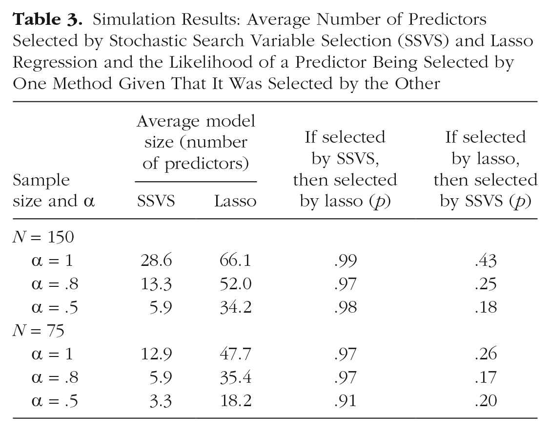
The average number of predictors selected by each method is summarized in Table 3. In all conditions, the lasso selected more predictors than SSVS, but the pattern of effects across conditions was similar. For both SSVS and the lasso, more predictors were selected when the sample size was larger and when reliability was higher. The predictors included by SSVS were largely a subset of the lasso predictors: Specifically, 91% to 99% of the predictors selected by the lasso were also selected by SSVS, whereas 17% to 43% of the predictors chosen by the lasso were also chosen by SSVS (see Table 3).

Table 3.

Simulation Results: Average Number of Predictors Selected by Stochastic Search Variable Selection (SSVS) and Lasso Regression and the Likelihood of a Predictor Being Selected by One Method Given That It Was Selected by the Other

Sample size and α	Average model size (number of predictors)		If selected by SSVS, then selected by lasso (p)	If selected by lasso, then selected by SSVS (p)
Sample size and α	SSVS	Lasso	If selected by SSVS, then selected by lasso (p)	If selected by lasso, then selected by SSVS (p)
N = 150
α = 1	28.6	66.1	.99	.43
α = .8	13.3	52.0	.97	.25
α = .5	5.9	34.2	.98	.18
N = 75
α = 1	12.9	47.7	.97	.26
α = .8	5.9	35.4	.97	.17
α = .5	3.3	18.2	.91	.20

To inspect the stability of which predictors were selected, and how this was affected by sample size and reliability of the outcome, we plotted the proportion of replications in which each of the 75 predictors was selected (see Fig. 5). For SSVS, the concentrations near zero show that most predictors were selected infrequently; however, some predictors were selected often. The number of predictors that were selected frequently increased as sample size and reliability increased. For example, in the most favorable condition (i.e., perfect reliability and N = 150), 12 predictors were selected in more than 90% of replications, and 38 predictors were selected in fewer than 25%. By comparison, for the sample size of 75 and perfect reliability, only 2 predictors were selected in more than 90% of the replications, and most predictors (59) were selected in fewer than 25%. The corresponding plots for the lasso show that in the condition with perfect reliability and a sample size of 150, most predictors (60) were selected in more than 90% of the replications. With perfect reliability but a sample size of 75, 23 were selected in more than 90%.

Fig. 5.

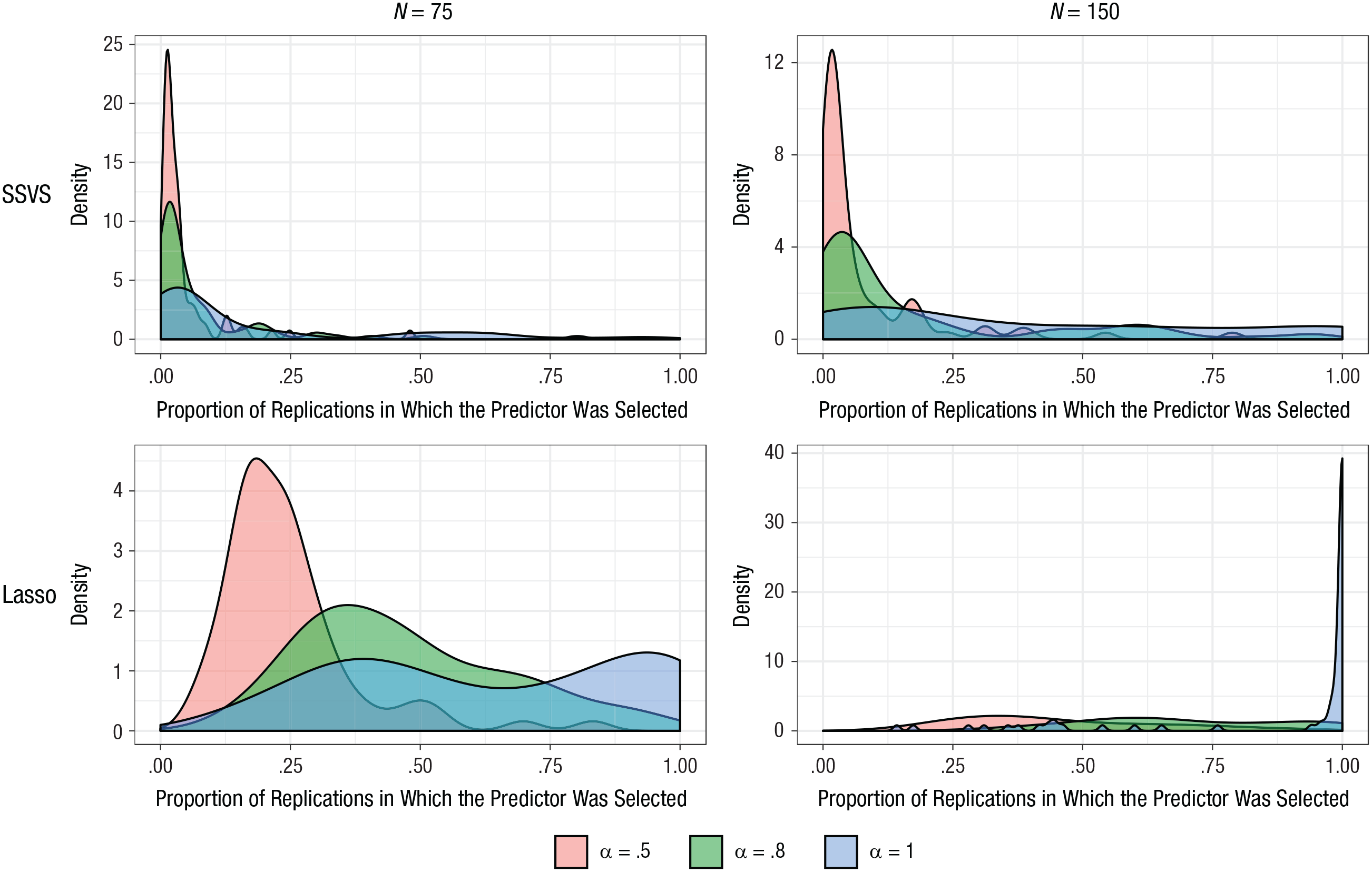
Simulation results: the effect of sample size and reliability of the outcome on the frequency with which each predictor was selected. Results for stochastic search variable selection (SSVS) and the lasso are in the top and bottom rows, respectively; results for a sample size of 75 are shown on the left, and results for a sample size of 150 are shown on the right. Each graph presents results for three different reliabilities (α = .5, .8, and 1).

Overall, our simulation supports previous work showing that the lasso and SSVS are related (Yuan & Lin, 2005). In the conditions studied, the lasso selected a larger set of predictors compared with SSVS, and SSVS generally selected a subset of the predictors that the lasso selected. Different population models are likely to lead to different results. In our example, the predictors identified from our theoretical model were moderately correlated. The elastic net (Zou & Hastie, 2005) is designed to perform well when predictors are highly correlated, but in our experience (results not reported here), the elastic net results in very few predictors being selected (none, one, or two). Again, we believe that SSVS is useful for the type of research problem illustrated by our focal example because the continuous information about predictors’ importance that SSVS provides can be used for variable selection. The predictors chosen in our simulation were fairly stable across the two models, and fewer predictors were selected with smaller samples sizes and lower reliability.

Discussion and Conclusion

Variable-selection problems arise frequently in psychology, and we have endeavored to show that SSVS is much more appropriate and useful than selecting predictors on the basis of the size or significance of bivariate correlations. As our example demonstrates, because SSVS selects predictors while accounting for uncertainty in which other variables are included in the model, variables selected by this approach are more likely to reliably predict the outcome.

In our example of selecting a set of predictors of pain unpleasantness, both bivariate selection and SSVS resulted in models with significant predictors related to stressful life events (discrimination), beliefs about pain and illness, and responses to pain (catastrophizing). However, in addition to explaining more (13%) unique variance in pain unpleasantness than the bivariate selection model, the SSVS model included a significant neurobiological predictor of pain unpleasantness, mean activity in the vmPFC, whereas the bivariate selection model did not include any neurobiological predictors. As the vmPFC has been particularly implicated in encoding pain unpleasantness (Price, 2000), the SSVS model is consistent with the pain literature and adds to current understanding of relationships between sociocultural and neurobiological mechanisms underlying the affective aspects of the pain experience.

The SSVS formulation we have presented here is one of a large family of related Bayesian variable-selection approaches. This approach may become computationally intractable as the number of predictors or sample size increases or when the predictors are highly intercorrelated (Yuan & Lin, 2005). It will be important for future simulation experiments to reveal where these limits lie for conditions representative of psychological data, so that extensions can be developed. Extensions have already been developed in other fields for different large-scale problems with many thousands of predictors (Fridley, 2009; Ishwaran & Rao, 2005).

Finally, although SSVS is a useful approach to variable selection, providing new information about the relative importance of predictors, it is a data-driven tool. If sufficient information is available to narrow down the set of predictors a priori, a more theory-driven approach should be preferred. In our example, all of the predictors for which data were collected made sense from a theoretical standpoint. This exploratory approach may also be especially useful for generating hypotheses or analyzing pilot data and then following up with new primary data collection. We believe that the information SSVS provides is useful not for automated decision making, but for thoughtfully condensing the predictor set.

Supplemental Material

Bainter_AMPPSOpenPracticesDisclosure-v1.0 – Supplemental material for Improving Practices for Selecting a Subset of Important Predictors in Psychology: An Application to Predicting Pain

Supplemental material, Bainter_AMPPSOpenPracticesDisclosure-v1.0 for Improving Practices for Selecting a Subset of Important Predictors in Psychology: An Application to Predicting Pain by Sierra A. Bainter, Thomas G. McCauley, Tor Wager and Elizabeth A. Reynolds Losin in Advances in Methods and Practices in Psychological Science

Supplemental Material

Bainter_Final_Supplementary_Methods – Supplemental material for Improving Practices for Selecting a Subset of Important Predictors in Psychology: An Application to Predicting Pain

Supplemental material, Bainter_Final_Supplementary_Methods for Improving Practices for Selecting a Subset of Important Predictors in Psychology: An Application to Predicting Pain by Sierra A. Bainter, Thomas G. McCauley, Tor Wager and Elizabeth A. Reynolds Losin in Advances in Methods and Practices in Psychological Science

Footnotes

Transparency

Action Editor: Frederick L. Oswald

Editor: Daniel J. Simons

Author Contributions

E. A. R. Losin generated the research question for the focal example and S. A. Bainter designed the analysis strategy. E. A. R. Losin and T. Wager designed the study and collected the data used in the focal example. S. A. Bainter and T. G. McCauley wrote the analysis code and analyzed the data. T. G. McCauley developed the shiny application. S. A. Bainter and E. A. R. Losin wrote the first draft of the manuscript. All the authors edited the manuscript and approved the final submitted version.

ORCID iD

Sierra A. Bainter

Supplemental Material

Additional supporting information can be found at

Notes

References

Anderson

K. O.

Green

C. R.

Payne

(2009). Racial and ethnic disparities in pain: Causes and consequences of unequal care. Journal of Pain, 10, 1187–1204. doi:10.1016/j.jpain.2009.10.002

Anderson

S. R.

Losin

E. A. R.

(2017). A sociocultural neuroscience approach to pain. Culture and Brain, 5, 14–35.

Baliki

M. N.

Petre

Torbey

Herrmann

K. M.

Huang

Schnitzer

T. J.

. . . Apkarian

A. V.

(2012). Corticostriatal functional connectivity predicts transition to chronic back pain. Nature Neuroscience, 15, 1117–1119.

Belloni

Chernozhukov

(2013). Least squares after model selection in high-dimensional sparse models. Bernoulli, 19, 521–547. doi:10.3150/11-BEJ410

Braun

M. T.

Converse

P. D.

Oswald

F. L.

(2019). The accuracy of dominance analysis as a metric to assess relative importance: The joint impact of sampling error variance and measurement unreliability. Journal of Applied Psychology, 104, 593–602. doi:10.1037/apl0000361

Budescu

D. V.

(1993). Dominance analysis: A new approach to the problem of relative importance of predictors in multiple regression. Psychological Bulletin, 114, 542–551. doi:10.1037/0033-2909.114.3.542

Chang

Cheng

Allaire

J. J.

Xie

McPherson

(2018). shiny: Web application framework for R (R package Version 1.2.0) [Computer software]. Retrieved from https://CRAN.R-project.org/package=shiny

Cheraghi

Nedjat

Mirmiran

Moslehi

Mansournia

Etminan

. . . McCandless

L. C.

(2018). Effects of food items and related nutrients on metabolic syndrome using Bayesian multilevel modelling using the Tehran Lipid and Glucose Study (TLGS): A cohort study. BMJ Open, 8(12), Article e020642. doi:10.1136/bmjopen-2017-020642

Efron

Hastie

Johnstone

Tibshirani

(2004). Least angle regression. The Annals of Statistics, 32, 407–499. https://doi.org/10.1214/009053604000000067

10.

Fragoso

T. M.

Bertoli

Louzada

(2018). Bayesian model averaging: A systematic review and conceptual classification. International Statistical Review, 86, 1–28. doi:10.1111/insr.12243

11.

Fridley

B. L.

(2009). Bayesian variable and model selection methods for genetic association studies. Genetic Epidemiology, 33, 27–37. doi:10.1002/gepi.20353

12.

Friedman

J. H.

Hastie

Tibshirani

(2010). Regularization paths for generalized linear models via coordinate descent. Journal of Statistical Software, 33(1).

13.

George

E. I.

McCulloch

R. E.

(1993). Variable selection via Gibbs sampling. Journal of the American Statistical Association, 88, 881–889.

14.

George

E. I.

McCulloch

R. E.

(1997). Approaches for Bayesian variable selection. Statistica Sinica, 7, 339–373.

15.

Grömping

(2015). Variable importance in regression models. Wiley Interdisciplinary Reviews: Computational Statistics, 7, 137–152. doi:10.1002/wics.1346

16.

Guan

Stephens

(2011). Bayesian variable selection regression for genome-wide association studies and other large-scale problems. The Annals of Applied Statistics, 5, 1780–1815.

17.

Hastie

Tibshirani

Friedman

J. H.

(2009). The elements of statistical learning: Data mining, inference, and prediction (2nd ed.). New York, NY: Springer.

18.

Henderson

D. A.

Denison

D. R.

(1989). Stepwise regression in social and psychological research. Psychological Reports, 64, 251–257. doi:10.2466/pr0.1989.64.1.251

19.

Ishwaran

Rao

J. S.

(2005). Spike and slab gene selection for multigroup microarray data. Journal of the American Statistical Association, 100, 764–780. doi:10.1198/016214505000000051

20.

Kim

H. J.

Yang

G. S.

Greenspan

J. D.

Downton

K. D.

Griffith

K. A.

Renn

C. L.

. . . Dorsey

S. G.

(2017). Racial and ethnic differences in experimental pain sensitivity: Systematic review and meta-analysis. Pain, 158, 194–211. doi:10.1097/j.pain.0000000000000731

21.

Lahiri

(Ed.). (2001). Model selection. Beachwood, OH: Institute of Mathematical Statistics.

22.

Lavie

Herer

Peled

Berger

Yoffe

Zomer

Rubin

A.-H. E.

(1995). Mortality in sleep apnea patients: A multivariate analysis of risk factors. Sleep, 18, 149–157. doi:10.1093/sleep/18.3.149

23.

Lee

K. E.

Sha

Dougherty

E. R.

Vannucci

Mallick

B. K.

(2003). Gene selection: A Bayesian variable selection approach. Bioinformatics, 19, 90–97.

24.

McNeish

D. M.

(2015). Using Lasso for predictor selection and to assuage overfitting: A method long overlooked in behavioral sciences. Multivariate Behavioral Research, 50, 471–484. doi:10.1080/00273171.2015.1036965

25.

O’Hara

R. B.

Sillanpää

M. J.

(2009). A review of Bayesian variable selection methods: What, how and which. Bayesian Analysis, 4, 85–117. doi:10.1214/09-BA403

26.

Olejnik

Mills

Keselman

(2000). Using Wherry’s adjusted R2 and Mallow’s Cp for model selection from all possible regressions. Journal of Experimental Education, 68, 365–380. doi:10.1080/00220970009600643

27.

Price

D. D.

(2000). Psychological and neural mechanisms of the affective dimension of pain. Science, 288, 1769–1772.

28.

R Core Team. (2017). R: A language and environment for sta-tistical computing. Vienna, Austria: R Foundation for Statistical Computing.

29.

Reich

(2014). [R code for a stochastic search variable selection]. Retrieved from https://www4.stat.ncsu.edu/~reich/ST740/code/SSVS_BMA.R

30.

Safren

S. A.

Hughes

J. P.

Mimiaga

M. J.

Moore

A. T.

Friedman

R. K.

Srithanaviboonchai

. . . Mayer

K. H.

, for the HPTN063 Study Team. (2016). Frequency and predictors of estimated HIV transmissions and bacterial STI acquisition among HIV-positive patients in HIV care across three continents. Journal of the International AIDS Society, 19, Article 21096. doi:10.7448/IAS.19.1.21096

31.

Sala-I-Martin

Doppelhofer

Miller

R. I.

(2004). Determinants of long-term growth: A Bayesian averaging of classical estimates (BACE) approach. American Economic Review, 94, 813–835.

32.

Schultz

Z. I.

Crook

Meloche

R. G.

Berkowitz

Milner

Zuberbier

A. O.

Meloche

(2004). Psychosocial factors predictive of occupational low back disability: Towards development of a return-to-work model. Pain, 107, 77–85. doi:10.1016/j.pain.2003.09.019

33.

Scott

S. L.

(2018). BoomSpikeSlab: MCMC for spike and slab regression (R package Version 1.0.0) [Computer software]. Retrieved from https://CRAN.R-project.org/package=BoomSpikeSlab

34.

Shiomi

(1978). Relations of pain threshold and pain tolerance in cold water with scores on Maudsley Personality Inventory and Manifest Anxiety Scale. Perceptual and Motor Skills, 47, 1155–1158.

35.

Srivastava

Chen

(2009). Comparison between the stochastic search variable selection and the least absolute shrinkage and selection operator for genome-wide association studies of rheumatoid arthritis. BMC Proceedings, 3, Article S21. doi:10.1186/1753-6561-3-S7-S21

36.

Swartz

M. D.

Kimmel

Mueller

Amos

C. I.

(2006). Stochastic search gene suggestion: A Bayesian hierarchical model for gene mapping. Biometrics, 62, 495–503.

37.

Swartz

M. D.

Peterson

C. B.

Lupo

P. J.

Forman

M. R.

Spitz

M. R.

. . . Shete

(2013). Investigating multiple candidate genes and nutrients in the folate metabolism pathway to detect genetic and nutritional risk factors for lung cancer. PLOS ONE, 8(1), Article e53475. doi:10.1371/journal.pone.0053475

38.

Swartz

M. D.

R. K.

Shete

(2008). Finding factors influencing risk: Comparing Bayesian stochastic search and standard variable selection methods applied to logistic regression models of cases and controls. Statistics in Medicine, 27, 6158–6174. doi:10.1002/sim.3434

39.

Thompson

(1995). Stepwise regression and stepwise discriminant analysis need not apply here: A guidelines editorial. Educational and Psychological Measurement, 55, 525–534. doi:10.1177/0013164495055004001

40.

Tibshirani

(1996). Regression shrinkage and selection via the lasso. Journal of the Royal Statistical Society: Series B (Methodological), 58, 267–288.

41.

Viallefont

Raftery

A. E.

Richardson

(2001). Variable selection and Bayesian model averaging in case-control studies. Statistics in Medicine, 20, 3215–3230. doi:10.1002/sim.976

42.

Wager

T. D.

Atlas

L. Y.

Lindquist

M. A.

Roy

Woo

C.-W.

Kross

(2013). An fMRI-based neurologic signature of physical pain. New England Journal of Medicine, 368, 1388–1397.

43.

Wickham

(2016). ggplot2: Elegant graphics for data analysis (2nd ed.). Cham, Switzerland: Springer.

44.

Yuan

Lin

(2005). Efficient empirical Bayes variable selection and estimation in linear models. Journal of the American Statistical Association, 100, 1215–1225. doi:10.1198/016214505000000367

45.

Zou

Hastie

(2005). Regularization and variable selection via the elastic net. Journal of the Royal Statistical Society: Series B (Statistical Methodology), 67, 301–320. doi:10.1111/j.1467-9868.2005.00503.x

Supplementary Material

Please find the following supplemental material available below.

For Open Access articles published under a Creative Commons License, all supplemental material carries the same license as the article it is associated with.

For non-Open Access articles published, all supplemental material carries a non-exclusive license, and permission requests for re-use of supplemental material or any part of supplemental material shall be sent directly to the copyright owner as specified in the copyright notice associated with the article.

0.00 MB

0.65 MB

0.07 MB