Sage Journals: Discover world-class research

Abstract

Ordinal variables, although extremely common in psychology, are almost exclusively analyzed with statistical models that falsely assume them to be metric. This practice can lead to distorted effect-size estimates, inflated error rates, and other problems. We argue for the application of ordinal models that make appropriate assumptions about the variables under study. In this Tutorial, we first explain the three major classes of ordinal models: the cumulative, sequential, and adjacent-category models. We then show how to fit ordinal models in a fully Bayesian framework with the R package brms, using data sets on opinions about stem-cell research and time courses of marriage. The appendices provide detailed mathematical derivations of the models and a discussion of censored ordinal models. Compared with metric models, ordinal models provide better theoretical interpretation and numerical inference from ordinal data, and we recommend their widespread adoption in psychology.

Keywords

ordinal models Likert items brms R open data open materials

Researchers refer to a variable as an ordinal variable when its categories have a natural order (Stevens, 1946). For example, peoples’ opinions are often probed using items with the following response options: “completely disagree,” “moderately disagree,” “moderately agree,” or “completely agree.” Such ordinal data are ubiquitous in psychology. Although it is widely recognized that ordinal data are not metric, it is commonplace to analyze them with methods that assume metric responses. However, this practice may lead to serious errors in inference (Liddell & Kruschke, 2018). This Tutorial provides a practical and straightforward solution to the perennial issue of analyzing ordinal variables with models that falsely assume the data are metric: flexible and easy-to-use Bayesian ordinal regression models implemented in the R statistical computing environment.

What, specifically, is wrong with analyzing ordinal data as if they were metric? This issue was examined in detail by Liddell and Kruschke (2018), whose arguments we summarize here. First, analyzing ordinal data with statistical models that assume metric variables, such as t tests and analysis of variance, can lead to low rates of correct detection, distorted effect-size estimates, inflated false alarm (Type I error) rates, and even inversions of differences between groups. There are three main reasons for these problems. First, and most important, the response categories of an ordinal variable may not be equidistant—an assumption that is required in statistical models of metric responses; rather, the psychological distance between adjacent response options may not be the same for all such pairs. For example, the difference between “completely disagree” and “moderately disagree” may be much smaller in a survey respondent’s mind than the difference between “moderately disagree” and “moderately agree.” Second, the distribution of ordinal responses may be nonnormal, particularly if very low or high values are frequently chosen. Third, variances of the unobserved variables that underlie the observed ordinal variables may differ between groups, conditions, time points, and so forth. Such unequal variances cannot be accounted for—or even detected, in some cases—with the ordinal-as-metric approach.

Although these potential pitfalls of applying metric models to ordinal data are widely known, the methods used to deal with them have not been sufficient. For example, one common approach has been to take averages over several Likert items and hope that this averaging makes the problems go away. Unfortunately, they do not. Because metric models fail to take into account these issues, and sometimes do not even indicate when there is a problem, we recommend adopting ordinal models instead. In order to determine whether a metric approximation of ordinal data is justified, researchers often have to apply an ordinal model, in which case they can use the results of this ordinal model regardless (Liddell and Kruschke, 2018).

Historically, appropriate methods for analyzing ordinal data were limited, although simple analyses, such as comparing two groups, could be performed with nonparametric approaches (Gibbons & Chakraborti, 2011). For more general analyses—regression-like methods, in particular—there were few alternatives to incorrectly treating ordinal data as either metric or nominal. However, using a metric or nominal model with ordinal data leads to over- or underestimating (respectively) the information provided by the data. Fortunately, recent advances in statistics and statistical software have provided many options for appropriate models of ordinal response variables. These methods are often referred to as ordinal regression models. Nevertheless, application of these methods remains limited, and the use of less appropriate metric models is widespread (Liddell & Kruschke, 2018).

Several reasons may underlie the persistent use of metric models for ordinal data: Researchers might not be aware of more appropriate methods, or they may hesitate to use them because of the perceived complexity in applying or interpreting them. Moreover, because closely related (or even the same) ordinal models are referred to with different names in different contexts, it may be difficult for researchers to decide which model is most relevant for their data and theoretical questions. Finally, researchers may also feel compelled to use “standard” analyses because journal editors and reviewers may be skeptical of any “nonstandard” approaches. Therefore, there is need for a review of and practical tutorial on ordinal models to facilitate their use in psychological research. This Tutorial provides such a review and guidance.

The structure of this article is as follows. First, we introduce three common classes of ordinal models. Next, we use two real-world data sets to provide a practical tutorial on fitting ordinal models in the R statistical computing environment (R Core Team, 2017). In the Conclusion, we counter possible objections to using ordinal models and provide practical guidelines on selecting the appropriate models for different research questions and data sets. In two appendices, we provide detailed mathematical derivations and theoretical interpretations of the ordinal models and an extension of ordinal models to censored data. We hope that the novel examples, derivations, unifying notation, and software implementation will allow readers to better address their research questions involving ordinal data.

Classes of Ordinal Models

A large number of parametric ordinal models can be found in the literature. Confusingly, they all have their own names, and their interrelations are often unclear. Fortunately, the vast majority of these models can be categorized within three distinct model classes (Mellenbergh, 1995; Molenaar, 1983; Van Der Ark, 2001): cumulative models, sequential models, and adjacent-category models. We begin by explaining the rationale behind these model classes in sufficient detail to allow researchers to use them and decide which best fits their research question and data. Detailed mathematical derivations and discussions are provided in Appendix A.

Cumulative models

For concreteness, we introduce the class of cumulative models in the context of an example data set of opinions about funding stem-cell research. The data set is part of the 2006 U.S. General Social Survey (http://gss.norc.org/) and contains, in addition to opinion ratings, a variable indicating the fundamentalism/liberalism of respondents’ religious beliefs. For our example (taken from Agresti, 2010), we analyze the extent to which religious belief predicts opinions about whether the government should fund stem-cell research, the ordinal dependent variable. The four levels of this Likert item are “definitely not fund” (1), “probably not fund” (2), “probably fund” (3), and “definitely fund” (4).¹ This is an ordinal variable because the categories have an ordering, but it is not known what the psychological distance between them is or whether the distances between categories are the same across participants. The assumptions of linear models are violated because the dependent variable cannot be assumed to be continuous or normally distributed. Therefore, we apply an ordinal model to these data, which are summarized in Table 1.

Table 1.

Frequencies of Opinion Ratings in the Stem-Cell Data Set

	Opinion rating^a
Religious belief	1	2	3	4
Fundamentalist	40	54	119	55
Moderate	25	41	135	71
Liberal	23	31	113	122

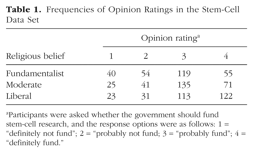
Participants were asked whether the government should fund stem-cell research, and the response options were as follows: 1 = “definitely not fund”; 2 = “probably not fund; 3 = “probably fund”; 4 = “definitely fund.”

Our cumulative model assumes that the observed ordinal variable Y, the opinion rating, originates from the categorization of a latent (not observable) continuous variable $\tilde{Y}$ . In this example, $\tilde{Y}$ is the latent opinion about funding stem-cell research. To model this categorization process, the model assumes that there are K thresholds $τ_{k}$ , which partition $\tilde{Y}$ into K + 1 observable, ordered categories of Y. In this example, there are four (K + 1 = 4) response categories, and therefore three (K = 3) thresholds. If we assume $\tilde{Y}$ to have a certain distribution (e.g., a normal distribution) with cumulative distribution function F, we can write the probability of Y being equal to category k as

\Pr (Y = k) = F (τ_{k}) - F (τ_{k - 1}) .

(1)

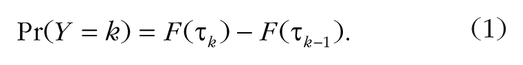
A conceptual illustration of this idea is shown in the top panel of Figure 1. To make this example more concrete, let us suppose we are interested in the probability of k = 2 (“probably not fund”) and have $τ_{1} = - 1$ as well as $τ_{2} = 1$ . Further, we assume $\tilde{Y}$ to be normally distributed with a standard deviation fixed to 1, and we call the corresponding cumulative normal distribution function $Φ$ (see Fig. A1 in Appendix A for a graph comparing this function with other common functions). Then, we compute

\begin{array}{l} \Pr (Y = 2) = Φ (τ_{2}) - Φ (τ_{1}) = Φ (1) - Φ (- 1) \\ = . 84 - . 16 = . 68 . \end{array}

(2)

Fig. 1.

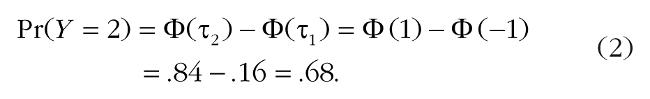
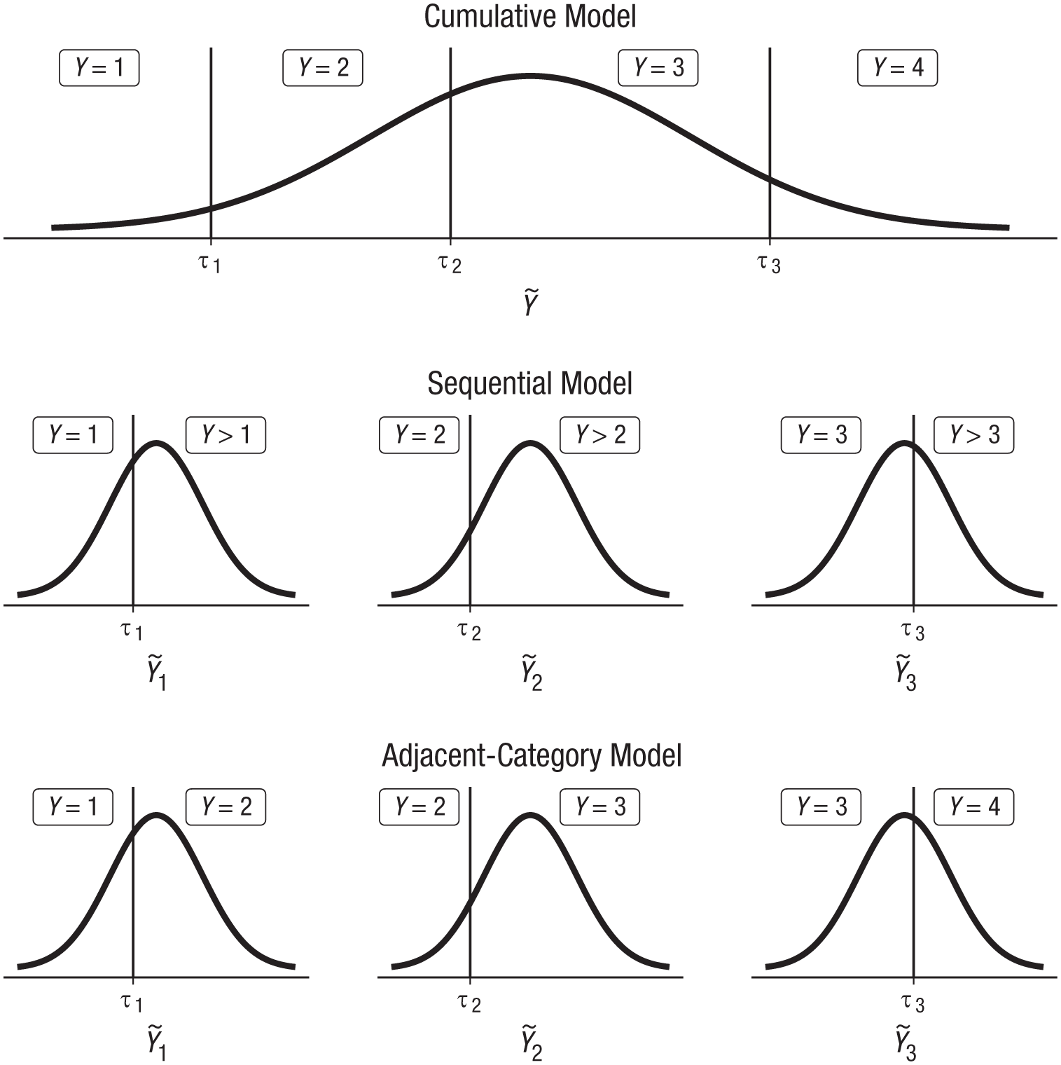
Illustration of the assumptions of the classes of ordinal models: cumulative models, sequential models, and adjacent-category models. Each type of model divides the latent continuous variable, $\tilde{Y}$ , into bins according to thresholds $τ$ . The area under the curve in each bin represents the probability of the corresponding event (observed ordinal response Y) given the set of possible events for the latent variable. (See the main text and Appendix A for more detailed descriptions of these three model classes.)

However, Equation 2 does not yet describe a regression model, because there are no predictor variables. We therefore formulate a linear regression for $\tilde{Y}$ with predictor term $η$ = b₁x₁ + b₂x₂ + . . ., so that $\tilde{Y}$ = $η + ε$ , where $ε$ describes the error term of the regression. Consequently, $\tilde{Y}$ is split into two parts. The first one (η) represents variation in $\tilde{Y}$ that can be explained by the predictors, and the second one (ε) represents variation that remains unexplained. Note that there is no intercept in the predictor term, because the thresholds $τ_{k}$ replace the model’s intercept, as the thresholds and intercept are not identified at the same time. Thus, we model the probabilities of Y being equal to category k given the linear predictor η:

\Pr (Y = k | η) = F (τ_{k} - η) - F (τ_{k - 1} - η) .

(3)

We provide a more detailed description and derivation of the general cumulative model in Appendix A.

The categorization interpretation is natural for many Likert-item data sets, in which ordered verbal (or numerical) labels are used to obtain discrete responses about a possibly continuous psychological variable. Given the widespread use of Likert items in psychology, cumulative models are possibly the most important class of ordinal models for psychological research. It is reasonable to assume that the stem-cell opinion ratings result from categorization of a latent continuous variable—the individual’s opinion about stem-cell research. Therefore, a cumulative model is theoretically motivated and justified for the data in this example.

We wish to predict funding opinion $\tilde{Y}$ from religious belief, which has categories “moderate,” “liberal,” and “fundamentalist.” In the regression model, we use dummy coding with “moderate” as the reference category. Thus, we have two numerical predictor variables, x₁ and x₂, and the corresponding regression coefficients, b₁ and b₂, have the following interpretation: b₁ is the contrast between moderate and liberal religious belief, and b₂ is the contrast between moderate and fundamentalist religious belief. The regression model of individuals’ latent opinions about stem-cell research is thus

{\tilde{Y}}_{k} = η + ε = b_{1} x_{1} + b_{2} x_{2} + ε .

(4)

We assume the latent variable $\tilde{Y}$ (or, equivalently, the error term $ε$ ) to be normally distributed² with a standard deviation fixed to 1. As before, we call the corresponding cumulative normal distribution function $Φ$ . Then, the probability for each response category k can be computed as follows:

\Pr (Y = k) = Φ (τ_{k} - (b_{1} x_{1} + b_{2} x_{2})) - Φ (τ_{k - 1} - (b_{1} x_{1} + b_{2} x_{2})) .

(5)

The parameters to be estimated are the three thresholds, $τ_{1}$ to $τ_{3}$ , as well as the two regression coefficients, b₁ and b₂. In the next main section, we show how to fit this model in the R programming environment.

Sequential models

We introduce the class of sequential models in the context of a real-life data set concerning marriage duration. The data are from the 2013–2015 U.S. National Survey of Family Growth (NSFG; Centers for Disease Control and Prevention, n.d.), in which data about family life were gathered for more than 10,000 individuals. We focus on a sample of 1,597 women who had been married at least once in their life at the time of the survey. Inspired by Teachman (2011), who used the NSFG 1995 data, we are interested in predicting the duration, in years, of first marriage. For now, we consider only divorced couples in order to illustrate the main ideas of a sequential model. If we included nondivorced women in the data, their data would be called censored because the event (divorce) was not observed. Although sequential models can be used to model censored data, we defer this additional complexity to Appendix B. The first 10 rows of the data are shown in Table 2.

Table 2.

First 10 Rows of the Marriage Data From the 2013–2015 U.S. National Survey of Family Growth (Centers for Disease Control and Prevention, n.d.)

Couple (coded as ID)	Couple lived together before marriage? (coded as together)	Woman’s age at marriage (coded as age)	Duration of marriage (coded as years)	Divorced at time of survey (coded as divorced)
1	Yes	19	9	True
2	Yes	22	9	False
3	Yes	20	5	False
4	Yes	22	2	False
5	Yes	25	6	False
6	Yes	30	1	False
7	Yes	32	9	False
8	No	24	14	True
9	No	37	1	True
10	Yes	18	13	True

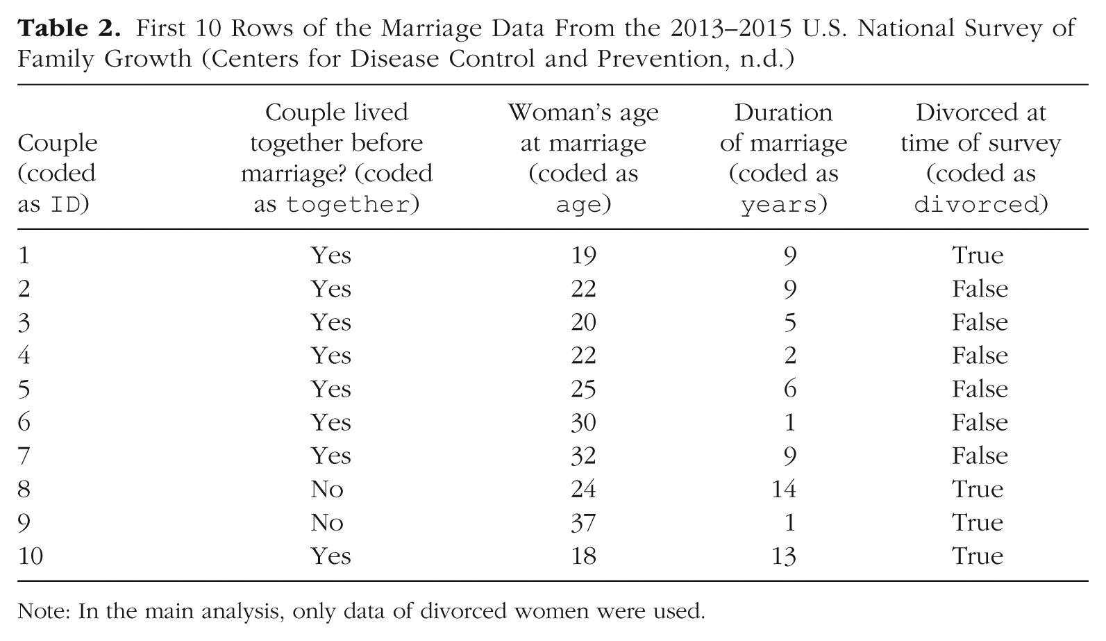
Note: In the main analysis, only data of divorced women were used.

For many ordinal variables, the assumption of a single underlying continuous variable, as in cumulative models, may not be appropriate. If the response can be understood as being the result of a sequential process, such that a higher response category is possible only after all lower categories are achieved, the sequential model proposed by Tutz (1990) is usually appropriate. For example, a couple can divorce in the 7th year only if they have not already divorced in their first 6 years of marriage: Duration of marriage in years—the ordinal dependent variable Y in the current example—can be thought of as resulting from a sequential process.

Sequential models assume that for every category k—year of marriage in our example—there is a latent continuous variable ${\tilde{Y}}_{k}$ that determines the transition between the kth and the k + 1th category. In the marriage example, ${\tilde{Y}}_{k}$ represents all the factors contributing to the probability of a couple’s marriage continuing beyond a given year k. Informally, we could call ${\tilde{Y}}_{k}$ “marriage quality” in this example. The categories are separated by thresholds $τ_{k}$ —perhaps thought of as the combination of all factors working against the marriage continuing beyond year k. If $\tilde{Y_{k}}$ is greater than the threshold τ_k, the sequential process—in this case, marriage—continues; otherwise, it stops at category k. The general concept underlying the class of sequential models is illustrated in the middle panel of Figure 1.

Because the thresholds $τ_{k}$ refer to different latent variables, they do not need to be ordered. That is, $τ_{k + 1}$ may be either greater than or less than $τ_{k}$ . Much as we did in the derivation of our cumulative model, we need to assume a certain distribution for $\tilde{Y_{k}}$ (e.g., a normal distribution) with cumulative distribution function F. Let us suppose we want to model the probability of divorce in the 3rd year. This means that divorce did not happen in the 1st year ( ${\tilde{Y}}_{1}$ > $τ_{1}$ ), did not happen in the 2nd year ( ${\tilde{Y}}_{2}$ > $τ_{2}$ ), but did happen in the 3rd year ( ${\tilde{Y}}_{3}$ ≤ $τ_{3}$ ). We can write this as follows:

\begin{array}{l} \Pr (Y = 3) = \Pr ({\tilde{Y}}_{1} > τ_{1}) \Pr ({\tilde{Y}}_{2} > τ_{2}) \Pr ({\tilde{Y}}_{3} \leq τ_{3}) \\ = (1 - \Pr ({\tilde{Y}}_{1} \leq τ_{1})) (1 - \Pr ({\tilde{Y}}_{2} \leq τ_{2})) \Pr ({\tilde{Y}}_{3} \leq τ_{3}) . \end{array}

(6)

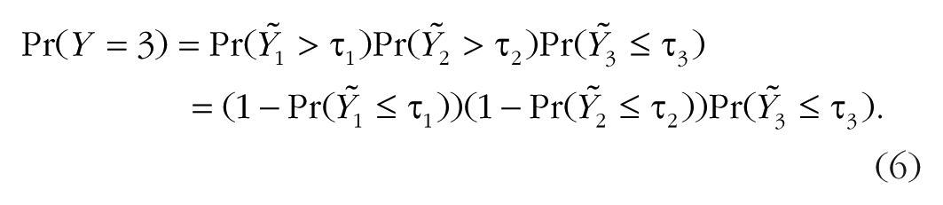
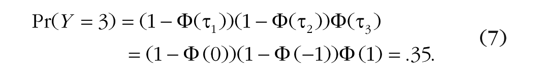
If we further assume Y₁, Y₂, and Y₃ to be standard normally distributed and set, just for illustration purposes, the threshold values as $τ_{1}$ = 0, $τ_{2}$ = −1, and $τ_{3}$ = 1, we can explicitly compute the probability of divorce in the 3rd year:

\begin{array}{l} \Pr (Y = 3) = (1 - Φ (τ_{1})) (1 - Φ (τ_{2})) Φ (τ_{3}) \\ = (1 - Φ (0)) (1 - Φ (- 1)) Φ (1) = . 35 . \end{array}

(7)

To make this sequential model an actual regression model, we set up a linear regression for each latent variable via ${\tilde{Y}}_{k} = η + ε_{k}$ , which includes a category-specific error term (i.e., $ε_{k}$ ). By default, all ${\tilde{Y}}_{k}$ share the same linear predictor $η$ , such that the effect of any potential predictor is constant across k (e.g., age at marriage is related to ${\tilde{Y}}_{k}$ identically for years k = 3 and k = 9.) This implies the following probability for category k:

\Pr (Y = k | η) = F (τ_{k} - η) \prod_{j = 1}^{k - 1} (1 - F (τ_{j} - η)) .

(8)

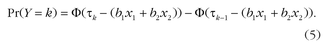
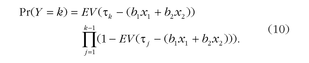
In words, the probability that Y falls in category k is equal to the probability that it did not fall in one of the former categories 1 to k – 1, multiplied by the probability that the sequential process stopped at k rather than continuing beyond it. In the current example, we use the survey respondents’ age at marriage and whether the couple was already living together before marriage as predictors of marriage duration. We can think of the years of marriage as a sequential process: Each year, the marriage may continue or end by divorce, but the latter can happen only if it did not happen before. The number of years of marriage until divorce is our response variable Y, whereas age at marriage and whether the couple was already living together before marriage are our predictor variables, which we denote as x₁ and x₂, respectively. As the latter predictor is categorical, for our analysis it is dummy coded as 1 if the couple was already living together and as 0 otherwise. This implies the following linear regression for the latent variables ${\tilde{Y}}_{k}$ :

{\tilde{Y}}_{k} = b_{1} x_{1} + b_{2} x_{2} + ε_{k} .

(9)

We assume an extreme-value distribution for ${\tilde{Y}}_{k}$ (F = EV), because it is the most common choice in discrete time-to-event, or survival, models. This function is graphically compared with other alternatives in Figure A1 in Appendix A. Together, these assumptions imply that the probability of a marriage ending in the kth year can be computed as follows:

\begin{array}{l} \Pr (Y = k) = E V (τ_{k} - (b_{1} x_{1} + b_{2} x_{2})) \\ \prod_{j = 1}^{k - 1} (1 - E V (τ_{j} - (b_{1} x_{1} + b_{2} x_{2}))) . \end{array}

(10)

For the current data set, the longest marriage ended in divorce after 27 years, so we have 26 thresholds ( $τ_{1}$ to $τ_{26}$ ) to estimate in addition to the two regression coefficients, b₁ and b₂. In the next main section, we show how to fit this model in the R programming environment.

Adjacent-category models

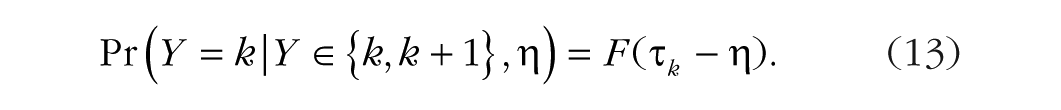
Adjacent-category models are widely used in item response theory and are applied in many large-scale assessment studies, such as the Program for International Student Assessment (PISA; OECD, 2017). They are somewhat different from cumulative and sequential models because it is difficult to think of a natural process leading to them. Therefore, an adjacent-category model can be chosen for its mathematical convenience rather than any quality of interpretation. Consequently, we do not present a practical example specifically dedicated to this approach, but we illustrate its use when we fit ordinal models to the stem-cell data set. Adjacent-category models predict the decision between two adjacent categories k and k + 1 using latent variables ${\tilde{Y}}_{k}$ , with thresholds $τ_{k}$ and cumulative distribution function F. If ${\tilde{Y}}_{k}$ < $τ_{k}$ , we choose category k; otherwise, we choose category k + 1. The decision process assumed by adjacent-category models is illustrated in the bottom panel of Figure 1. We can formally write this as follows:

\Pr (Y = k | Y \in {k, k + 1}) = F (τ_{k}) .

(11)

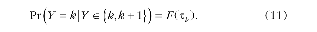
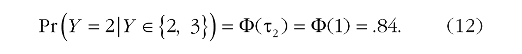
This is superficially similar to the form of sequential models, but with an important distinction. Sequential models model the decision between Y = k and Y > k, whereas adjacent-category models model the decision between Y = k and Y = k + 1. Suppose that the latent variable ${\tilde{Y}}_{2}$ is standard normally distributed (with distribution function $Φ$ ) and $τ_{2}$ = 1. In this case, the probability of choosing Y = 2 (“probably not fund”) over Y = 3 (“probably fund”) in the stem-cell example would be written as follows in an adjacent-category model:

\Pr (Y = 2 | Y \in {2, 3}) = Φ (τ_{2}) = Φ (1) = . 84 .

(12)

Including the linear predictor $η$ in this model leads to the following general equation:

\Pr (Y = k | Y \in {k, k + 1}, η) = F (τ_{k} - η) .

(13)

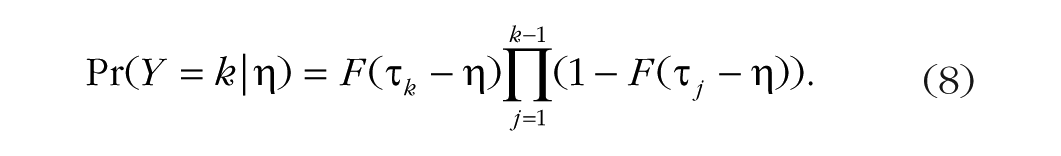
The (unconditional) probability of the response Y being equal to category k given $η$ (i.e., Pr(Y = k| $η$ )) is computed with a quite extensive formula, shown in Appendix A.

Generalizations of ordinal models

We have introduced the three most important classes of ordinal models and refer readers to Appendix A for more details on each of them. Box 1 provides an overview of these three model classes and how to apply them with the software package described in the next main section. However, before discussing how to fit ordinal models in R, we briefly consider generalizations of these model classes to handle category-specific effects and unequal variances.

Box 1. Overview of the Three Classes of Ordinal Models and How to Apply Them With brms Syntax

Consider an observed ordinal response variable Y and a predictor X. The three model classes can be summarized as follows:

1. Cumulative model

• Y originates from categorization of a latent variable $\tilde{Y}$ .

• Basic code for implementing a cumulative model: brm(Y $\sim$ X, family = cumulative(), …),

• Example: Using gender to predict responses to a 5-point Likert item

2. Sequential model

• Y is the result of a sequential process.

• Basic code for implementing a sequential model: brm(Y $\sim$ X, family = sratio(), …)

• Example: Using age to predict the number of cars people have bought

3. Adjacent-category model

• Y is modeled as the decision between two adjacent categories of $\tilde{Y}$ .

• Basic code for implementing an adjacent-category model: brm(Y $\sim$ X, family = acat(), …),

• Example: Predicting the number of correctly solved subitems in a complex math task

Generalizations of ordinal models

1. Category-specific effects can be modeled with sequential and adjacent-category models.

• Basic code for modeling category-specific effects: brm(Y $\sim$ cs(X), family = acat()/sratio(), …)

• Example: Using gender to predict responses to Likert items when gender is expected to affect responses high on the rating scale differently than responses low on the rating scale

2. Unequal variances can be modeled with all three classes of ordinal models.

• Basic code for modeling unequal variances: brm(bf(Y $\sim$ X, disc $\sim$ X), …)

• Example: Using gender to predict responses to Likert items when the variances of the latent variables differ between genders

Note: … indicates additional arguments to brm(), such as specifying a data set.

Category-specific effects

In all of the ordinal models we have described thus far, all predictors are by default assumed to have the same effect on all response categories, which may not always be an appropriate assumption. It is often possible that a predictor has different effects on different response categories of Y. For example, religious belief may have little relation to whether people choose “definitely not fund” over “probably not fund” in rating their opinion about funding stem-cell research, but may strongly predict whether they choose “probably fund” over “definitely fund.” In such a case, one can model the predictor as having category-specific effects by estimating not one but K coefficients for it. Doing so is unproblematic in sequential and adjacent-category models, but may lead to negative probabilities, and thus problems in model fitting, in cumulative models (see Appendix A).

Unequal variances

Especially in the context of cumu-lative models, the response function F is usually assumed to be a standard normal distribution, that is, to have a variance ν of 1 for reasons of model identification. Freely varying ν is not possible in ordinal models if all the thresholds $τ$ are allowed to vary as well. However, it is possible for ν to vary as a function of group, condition, time, or any other predictor variable (i.e., for $\tilde{Y}$ to have unequal variances across groups, conditions, etc.) provided that the baseline variance is fixed to some value. Ignoring the possibility of unequal variances can lead to problems such as inflated error rates and distorted effect sizes (Liddell & Kruschke, 2018). Fortunately, unequal variances are easily incorporated into the ordinal models, as we show later.

Disclosures

The complete R code for this Tutorial and the example data used here are available at the Open Science Framework (https://osf.io/cu8jv/).

Fitting Ordinal Models in R

Although a number of software packages in the R statistical programming environment (R Core Team, 2017) allow modeling ordinal responses, here we use the brms (Bayesian regression models using ‘Stan’) package (Bürkner, 2017, 2018; Carpenter et al., 2017), for two main reasons. First, it can estimate all three ordinal model classes we have introduced in combination with multilevel structures, category-specific effects (though not in the case of cumulative models), unequal variances, and more. Second, brms estimates models in a Bayesian framework, which provides considerably more information about the models and their parameters than the frequentist approach (Gelman et al., 2013; McElreath, 2016), allows a more natural quantification of uncertainty (Kruschke, 2014), and makes it possible to estimate models when traditional methods based on maximum likelihood fail (Eager & Roy, 2017). A brief description of the basic concepts of Bayesian statistics is provided in Box 2 (see also Kruschke & Liddell, 2018a, 2018b). We provide brief notes on implementing ordinal models using other software packages in our concluding section.

Box 2. Basics of Bayesian Statistics

Bayesian statistics focuses on the posterior distribution p(θ|Y), where θ are the model parameters (unknown quantities) and Y are the data (known quantities) to condition on. The posterior distribution is generally computed as $p (θ | Y) = \frac{p (Y | θ) p (θ)}{p (Y)} .$

In this equation, p(Y|θ) is the likelihood, p(θ) is the prior distribution, and p(Y) is the marginal likelihood. The likelihood p(Y|θ) is the distribution of the data given the parameters and thus relates the data to the parameters. The prior distribution p(θ) describes the uncertainty in the parameters before the data have been seen. It thus allows explicit incorporation of prior knowledge into the model. The marginal likelihood p(Y) serves as a normalizing constant so that the posterior is an actual probability distribution. Except in the context of specific methods (i.e., Bayes factors), p(Y) is rarely of direct interest.

In classical frequentist statistics, parameter estimates are obtained by finding those parameter values that maximize the likelihood. In contrast, Bayesian statistics estimate the full (joint) posterior distribution of the parameters. Estimating the full posterior distribution not only is fully consistent with probability theory, but also is much more informative than estimating a single point (with an approximate measure of uncertainty commonly known as standard error).

Obtaining the posterior distribution analytically is rarely possible, and thus Bayesian statistics relies on Markov-Chain Monte Carlo methods to obtain samples (i.e., random values) from the posterior distribution. Such sampling algorithms are computationally very intensive, and thus fitting models using Bayesian statistics is usually much slower than fitting models using frequentist statistics. However, the advantages of Bayesian statistics—such as greater modeling flexibility, inclusion of prior distributions, and more informative results—are often worth the increased computational cost.

In this section, we assume that readers know how to load data sets into R and execute other basic commands. Readers unfamiliar with R may consult free online R tutorials.³ To follow the examples in this section, users first need to install the brms R package. Packages should be installed only once, and therefore the following code snippet, which installs brms, should be run only once:

install.packages("brms")

In order to have the brms functions available in the current R session, users must load the package at the beginning of every session:

library(brms)

Next, we discuss analyses of two real-world data sets (from different areas of psychology) in which the main dependent variable is an ordinal variable. We remind readers that ordinal data are not limited to the types of variables discussed here, but can be found in a wide variety of research areas, as noted by Stevens (1946): “As a matter of fact, most of the scales used widely and effectively by psychologists are ordinal scales” (p. 679).

Opinions about funding stem-cell research

First, we analyze the stem-cell data set introduced earlier (see Table 1). We wish to predict the respondents’ opinions about funding stem-cell research (coded as rating) from the degree of fundamentalism of their religious beliefs (coded as belief). This model can easily be fitted by including three arguments in the brm() function, as follows:

fit_sc1 <- brm(

formula = rating ~ 1 + belief,

data = stemcell,

family = cumulative("probit")

)

The three arguments inside brm() are formula, data, and family, respectively. First, and perhaps most important, the formula argument identifies which variable (or variables) is the dependent variable, and which variable (or variables) is the predictor variable. The model’s formula is specified with standard R modeling syntax, in which dependent variables are written on the left-hand side of ~ and predictors are written on the right-hand side; predictors are separated by + unless an interaction between predictors is desired, in which case they are separated by inserting *, rather than +. The 1 on the right-hand side of ~ means that an intercept (i.e., the threshold in an ordinal model) should be included. Although it is included automatically, we added this notation here for clarity. Note also that arguments do not have to be named because R functions allow the arguments to be specified in order; if arguments are not named, they will be applied in the expected order.

In addition, this function includes data and family arguments. The former takes a data frame from the current R environment. The latter defines the distribution of the response variable, that is, the specific ordinal model to be used and the transformation to be applied to the predictor term—which is nothing other than the distribution function F in ordinal models. We have specified cumulative(“probit”) in order to apply a cumulative model assuming the latent variable (or, equivalently, the error term ε) to be normally distributed. If we had omitted probit from the specification of the family, the default logistic distribution would have been assumed instead (see Appendix A for a visualization).

The model (which we have saved into the fit_sc1 variable) is readily summarized via

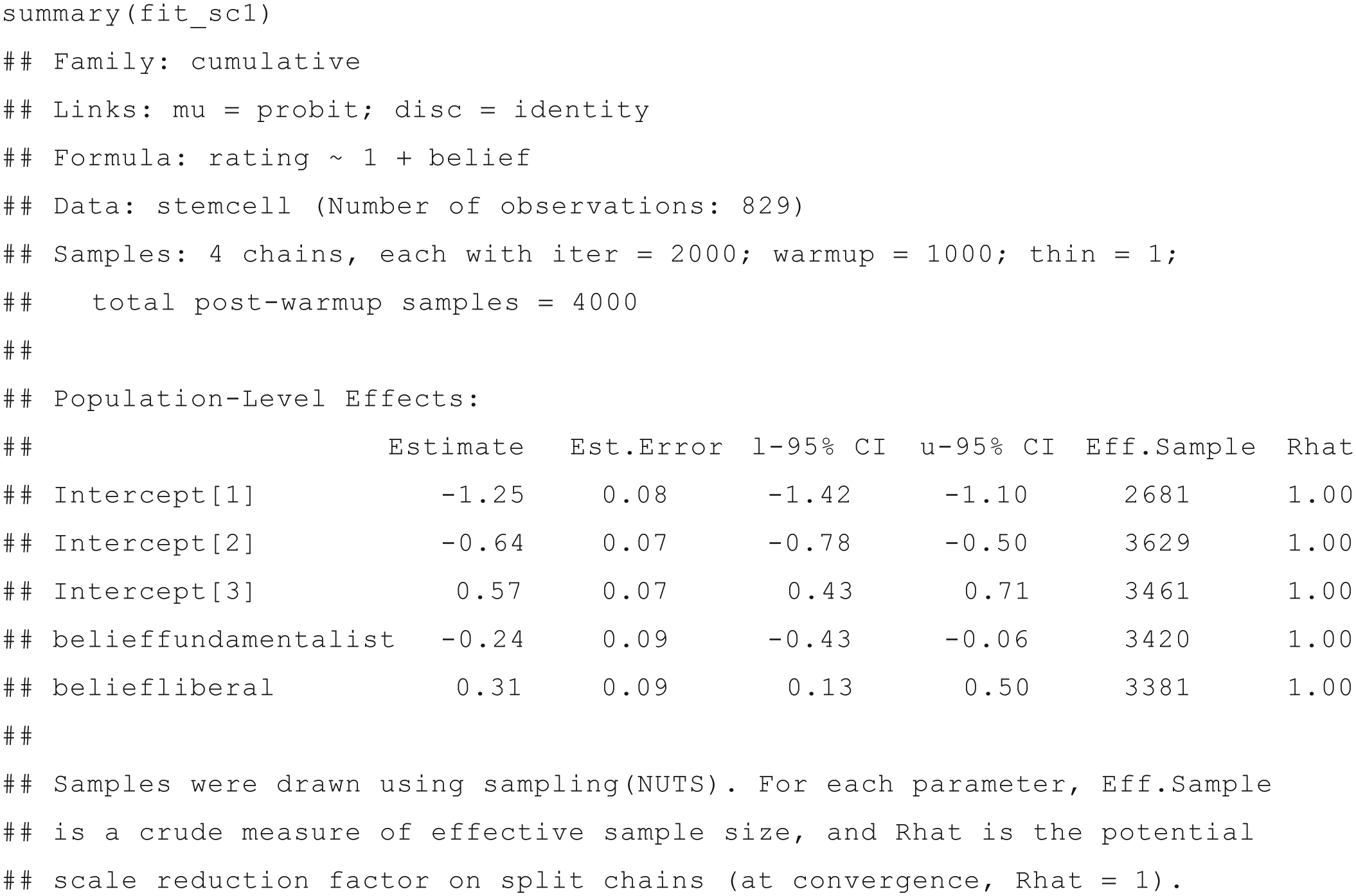
For consistency with other model classes that brms supports, thresholds in ordinal models are called “intercepts” although, from a theoretical perspective, they are not quite the same. In addition to the regression coefficients (which are displayed under the heading Population-Level Effects), this display includes information about the model (first three rows), the data, and the Bayesian estimation algorithm (Samples row; for additional information about this algorithm, see, e.g., Betancourt, 2017; Bürkner, 2017; van Ravenzwaaij, Cassey, & Brown, 2018).

Of most importance for present purposes are the regression coefficients. The Estimate column provides the posterior means of the parameters, and the Est.Error column shows the parameters’ posterior standard deviations. These quantities are analogous, but not identical, to frequentist point estimates and standard errors, respectively. The l-95% CI and u-95% CI columns provide the lower and upper bounds of the 95% credible intervals, or CIs, which are Bayesian confidence intervals (the numbers refer to the 2.5th and 97.5th percentiles of the posterior distributions). Although credible intervals can be numerically similar to their frequentist counterparts, confidence intervals, they actually lend themselves to an intuitive probabilistic interpretation, unlike confidence intervals, which are often mistakenly so interpreted (Hoekstra, Morey, Rouder, & Wagenmakers, 2014; Morey, Hoekstra, Rouder, Lee, & Wagenmakers, 2016). To get different credible intervals, one can use the prob argument (e.g., summary(fit_sc1, prob = .99) will yield 99% CIs).

The two additional columns, named Eff.Sample (effective sample size) and Rhat, indicate whether the model-fitting algorithm converged to the underlying values and are briefly explained in the last three rows of the output. In short, Rhat should not be larger than 1.1, and Eff.Sample should be as large as possible. For most applications, an effective sample size greater than 1,000 is sufficient for stable estimates. Because these quantities are not the focus of this Tutorial—and convergence is not a problem for any of the models considered here—we refer readers to Bürkner (2017) for more details.

The first three rows of the output under Population-Level Effects describe the three thresholds of the cumulative model as applied to the stem-cell opinion data. Recall that when the cumulative distribution function F is $Φ$ (standard normal distribution), $\tilde{Y}$ is a standard normal variable. Consequently, the thresholds indicate where the continuous latent variable $\tilde{Y}$ is partitioned to produce the observed responses Y, in standard-deviation units. Therefore, applying $Φ$ to each threshold leads to the cumulative probability of responses below that threshold if all predictor variables were zero. Although it is important to be able to interpret the thresholds, they are rarely of central focus in modeling (much as ordinary regression intercepts are rarely of central focus). Instead, we are most interested in the regression coefficients b₁ and b₂, to which we turn next.

Because religious belief was coded as a factor in R with “moderate” as the reference category, the coefficients belieffundamentalist and beliefliberal indicate the extent to which people with fundamentalist and liberal religious beliefs differed from those with moderate beliefs on the latent scale of opinion regarding funding stem-cell research. The point estimate of beliefliberal indicates that on the latent opinion scale, people with liberal beliefs held opinions that were 0.31 SD more positive toward funding stem-cell research compared with the opinions of moderates. The 95% CI of this parameter is between 0.13 and 0.50, and so does not include zero. We can therefore conclude with at least 95% probability that people with liberal religious beliefs held more positive opinions regarding the funding of stem-cell research than did people with moderate religious beliefs.

People with fundamentalist religious beliefs, on the other hand, had more negative opinions regarding funding stem-cell research than did people with moderate religious beliefs. On the latent opinion scale, fundamentalists’ opinions about funding stem-cell research were 0.24 SD more negative than the opinions of people with moderate religious beliefs. This parameter is between −0.43 and −0.06 with 95% probability.

The results can also be summarized visually by plotting the estimated relationship between religious belief and response to the opinion question. Figure 2 displays the estimated probabilities of the four response categories for the three religious-belief groups. It is quite clear from the figure that fundamentalists were less likely to respond “definitely fund” (4) than were either of the other two groups. Similarly, they were more likely to respond “definitely not fund” (1) and “probably not fund” (2) than the other two groups were. The code to produce this figure is as follows:

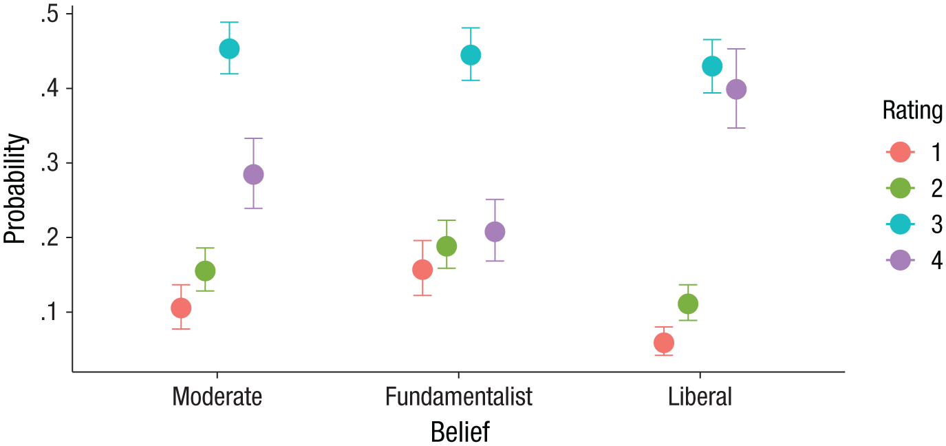
marginal_effects(fit_sc1, ‘belief’, categorical = TRUE)

Fig. 2.

Marginal effects of religious belief on opinion about funding stem-cell research, from model fit_sc1 (data from the 2006 U.S. General Social Survey, http://gss.norc.org/). The posterior mean estimate of the probability of responses in each opinion rating category is shown for each of the three groups (moderate, fundamentalist, and liberal). Error bars indicate 95% credible intervals.

Category-specific effects

Thus far, we assumed that the effect of religious belief was equal across the opinion rating categories. That is, there was only one predictor term for the effect of fundamentalist and liberal beliefs on funding opinion. However, this assumption may not be appropriate, and beliefs may affect opinions differently depending on the rating category. For example, it is possible that individuals with liberal beliefs are more likely to respond with the highest rating than are individuals with moderate beliefs, but that the two groups do not otherwise differ in their opinion ratings. When the effects of predictors can vary in this manner across categories, the resulting model is said to have category-specific effects.

Next, we consider whether religious belief has category-specific effects in this data set. In other words, does its relationship to funding opinion vary across response categories? Fitting category-specific effects in cumulative models is problematic because of the possibility of negative probabilities (see Appendix A) and consequently is not allowed in brms. Therefore, we use an adjacent-category model instead. To specify an adjacent-category model, we use family = acat() instead of family = cumulative() as an argument to the brm() function. Then, to model religious belief with possible category-specific effects, we wrap this variable in cs() in the model’s formula:

fit_sc2 <- brm(

formula = rating ^~ 1 + cs(belief),

data = stemcell,

family = acat("probit")

)

As indicated in Table 3, liberals preferred “definitely fund” (4) over “probably fund” (3) much more than moderates did, b = 0.45 (95% CI = [0.21, 0.68]). At the same time, there was little difference between liberals and moderates for the other response categories. In contrast, fundamentalists preferred lower response categories than moderates across the rating scale, but the differences were quite small and uncertain—as indicated by the rather wide 95% CIs, which also overlap zero.

Table 3.

Summary of the Regression Coefficients for the Category-Specific Adjacent-Category Model Fitted to the Stem-Cell Data Set

Predictor	Estimate	95% credible interval
First threshold (coded as Intercept[1])	−0.32	[–0.62, 0.01]
Second threshold (coded as Intercept[2])	−0.73	[–0.94, –0.52]
Third threshold (coded as Intercept[3])	0.40	[0.22, 0.58]
Fundamentalists’ vs. moderates’ preference for “2” over “1” (coded as belieffundamentalist[1])	−0.13	[–0.53, 0.28]
Fundamentalists’ vs. moderates’ preference for “3” over “2” (coded as belieffundamentalist[2])	−0.24	[–0.54, 0.04]
Fundamentalists’ vs. moderates’ preference for “4” over “3” (coded as belieffundamentalist[3])	−0.08	[–0.33, 0.19]
Liberals’ vs. moderates’ preference for “2” over “1” (coded as beliefliberal[1])	−0.12	[–0.57, 0.34]
Liberals’ vs. moderates’ preference for “3” over “2” (coded as beliefliberal[2])	0.06	[–0.25, 0.36]
Liberals’ vs. moderates’ preference for “4” over “3” (coded as beliefliberal[3])	0.45	[0.21, 0.68]

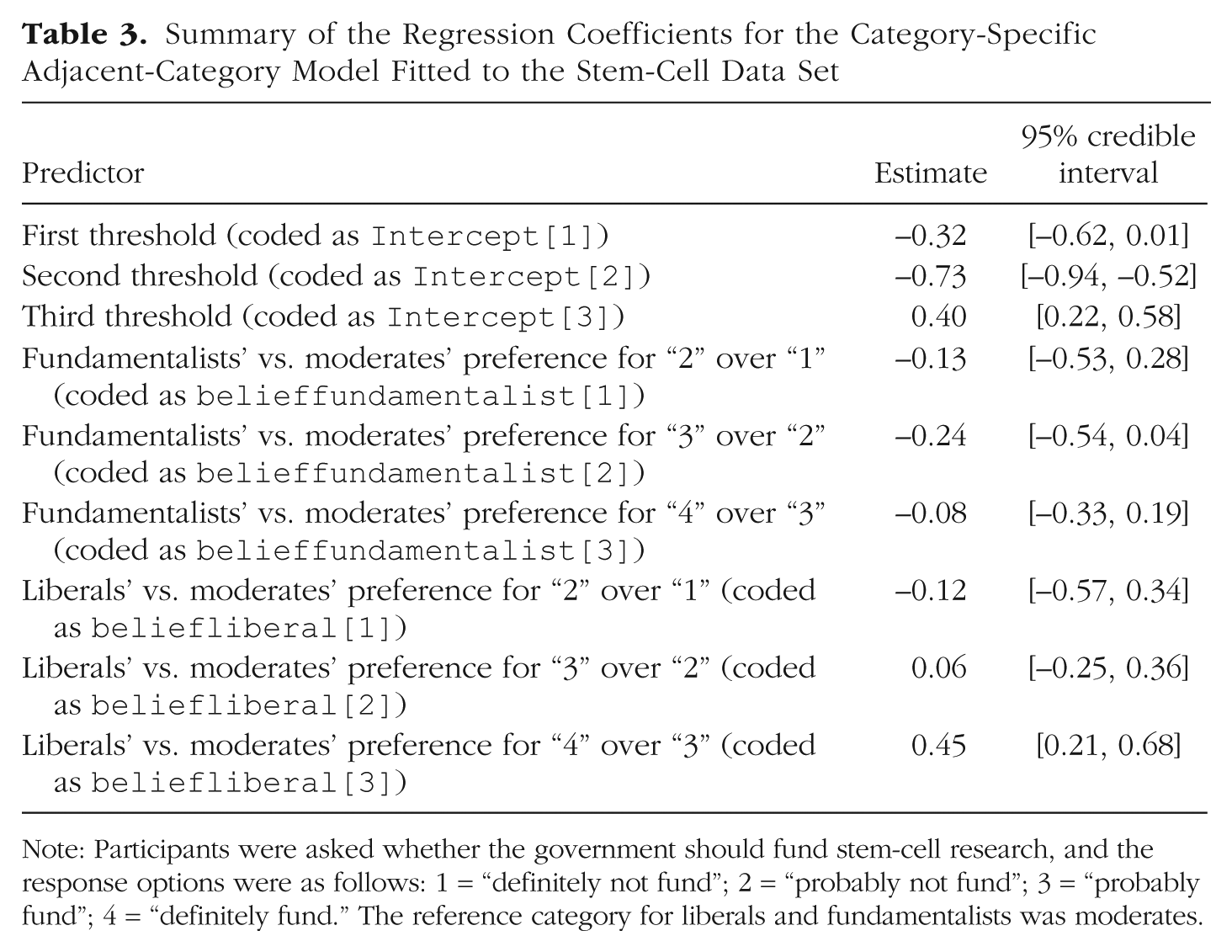
Note: Participants were asked whether the government should fund stem-cell research, and the response options were as follows: 1 = “definitely not fund”; 2 = “probably not fund”; 3 = “probably fund”; 4 = “definitely fund.” The reference category for liberals and fundamentalists was moderates.

It can be more difficult to interpret the sizes of coefficients from an adjacent-category model, compared with coefficients from a cumulative model. Thus, we recommend plotting an adjacent-category model’s predicted values (e.g., via marginal_effects(fit_sc2)), so that the magnitudes of the effects can be better understood. With the stem-cell data, the resulting figure looks very similar to Figure 2, and thus we do not show it here.

Unequal variances

As we noted earlier, it is usually assumed that the variance of the latent variable is the same throughout the model. Within the framework of ordinal models in brms, we can relax this assumption.⁴ For the stem-cell data, this implies asking whether the variances of funding opinions differ across categories of religious belief.

Conceptually, unequal variances are incorporated in the model by specifying an additional regression formula for the variance component of the latent variable $\tilde{Y}$ . In brms, the parameter related to latent variances is called disc (short for “discrimination”), following conventions in item response theory. Note that disc is not the variance itself, but the inverse of the standard deviation, s. That is, s = 1/disc. Further, because disc must be strictly positive, it is by default modeled on the log scale.

Predicting auxiliary parameters (parameters of the distribution other than the mean, or location) in brms is accomplished by passing multiple regression formulas to the brm() function. Each formula must first be wrapped in another function, bf() or lf() (for “linear formula”)—depending on whether it is a main or an auxiliary formula, respectively. The formulas are then combined and passed to the formula argument of brm(). Because the standard deviation of the latent variable is fixed to 1 for the baseline group (moderates), disc cannot be estimated for all three religious-belief groups. We must therefore ensure that disc is estimated only for the liberals and fundamentalists. To do so, we omit the intercept from the model of disc by writing 0 + … on the right-hand side of the regression formula. By default, R applies cell-mean coding to factors in formulas without an intercept. That would lead to disc being estimated for all three groups, so we must deactivate it via the cmc argument of lf(). With this in mind, an unequal-variances cumulative model of the stem-cell data is specified as follows:

fit_sc4 <- brm(

formula = bf(rating ~ 1 + belief) +

lf(disc ~ 0 + belief, cmc = FALSE),

data = stemcell,

family = cumulative("probit")

)

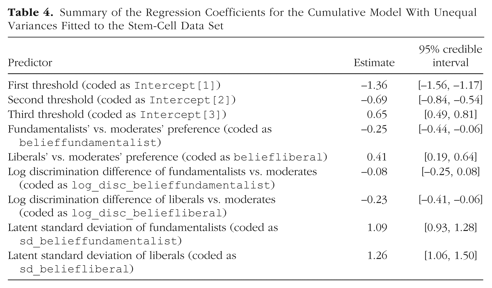
The syntax for specifying unequal variances is identical to the syntax of an equal-variances model with one important addition: A formula for the disc parameter is added, using a + between the formulas. This additional formula is wrapped in lf() to indicate that an auxiliary parameter, disc, is predicted.

The estimated parameters of the unequal-variances model are summarized in Table 4. Because disc is the inverse of the standard deviation of $\tilde{Y}$ , and by default is modeled through a log link, the model predicts log(disc) instead of disc. To also display the standard deviations, s, we transformed log(disc) to s with s = 1/exp(log(disc)).⁵ The standard deviation of the latent variable was higher for liberals (SD = 1.26, 95% CI = [1.06, 1.50]) than for moderates, for whom the standard deviation was fixed to 1. The standard deviation was also somewhat higher for fundamentalists (SD = 1.09, 95% CI = [0.93, 1.28]) than for moderates, although this difference was not substantial, nor did the 95% CI exclude 1. The regression coefficients for religious belief changed slightly compared with the coefficients in the equal-variances model; however, the main result that liberals tended to prefer more positive responses than moderates, and fundamentalists tended to prefer more negative responses than moderates, was similar to the main result of the equal-variances model.

Table 4.

Summary of the Regression Coefficients for the Cumulative Model With Unequal Variances Fitted to the Stem-Cell Data Set

Predictor	Estimate	95% credible interval
First threshold (coded as Intercept[1])	−1.36	[–1.56, –1.17]
Second threshold (coded as Intercept[2])	−0.69	[–0.84, –0.54]
Third threshold (coded as Intercept[3])	0.65	[0.49, 0.81]
Fundamentalists’ vs. moderates’ preference (coded as belieffundamentalist)	−0.25	[–0.44, –0.06]
Liberals’ vs. moderates’ preference (coded as beliefliberal)	0.41	[0.19, 0.64]
Log discrimination difference of fundamentalists vs. moderates (coded as log_disc_belieffundamentalist)	−0.08	[–0.25, 0.08]
Log discrimination difference of liberals vs. moderates (coded as log_disc_beliefliberal)	−0.23	[–0.41, –0.06]
Latent standard deviation of fundamentalists (coded as sd_belieffundamentalist)	1.09	[0.93, 1.28]
Latent standard deviation of liberals (coded as sd_beliefliberal)	1.26	[1.06, 1.50]

Model comparison

We have now fitted three different ordinal models to the stem-cell opinion data, and it is natural to ask which model we should choose to base our inference on. Many of the coefficients in the model with category-specific effects were rather small and uncertain, which suggests that category-specific effects may not be necessary. Similarly, the parameter estimates from the unequal-variances model suggest that the variances of fundamentalists’ and moderates’ opinions were quite similar, though liberals’ opinions were more variable. One formal approach to model comparison is to investigate the relative fit of computed models to the data, and one method to assess relative fit is approximate leave-one-out cross-validation (LOOCV; Vehtari, Gelman, & Gabry, 2017). LOOCV provides a score that can be interpreted in the same way as typical information criteria, such as Akaike’s information criterion (AIC; Akaike, 1998) or the Watanabe-Akaike information criterion (WAIC; Watanabe, 2010),⁶ in the sense that smaller values indicate better fit. Although a detailed exposition of this topic is beyond the scope of this article, we illustrate how to compare the relative fit of the three models we have discussed to the stem-cell data using LOOCV.

However, we also want to make sure that the differences between the equal-variances cumulative model (fit_sc1) and the adjacent-category model with category-specific effects (fit_sc2) are not due to the fact that the models belong to different classes of ordinal models. Therefore, we also fit an adjacent-category model without category-specific effects (fit_sc3); the syntax is the same as that for the model with these effects except that cs() is omitted, so we do not show the code here. The comparison between the four ordinal models using approximate LOOCV is done via

loo(fit_sc1, fit_sc2, fit_sc3, fit_sc4)

Tables 5 and 6 display the estimated LOO information criterion (LOOIC) for each model and the differences between the LOOICs for different models. As the tables show, the two cumulative models have a somewhat better fit (smaller LOOIC values) than the two adjacent-category models, although the differences are not very large (not more than about 1 or 2 times the corresponding standard error). The LOOIC values for the two adjacent-category models are very similar, which implies that estimating category-specific effects does not substantially improve model fit. Similarly, the unequal-variances cumulative model has only a slightly smaller LOOIC value than the equal-variances cumulative model; unequal variances improve model fit slightly, but the difference is not substantial.

Table 5.

Values of the Leave-One-Out Information Criterion (LOOIC) for the Four Ordinal Models of the Stem-Cell Data

Model	LOOIC	SE
fit_sc1	2,040.61	31.10
fit_sc2	2,042.80	31.49
fit_sc3	2,043.70	30.89
fit_sc4	2,039.04	31.22

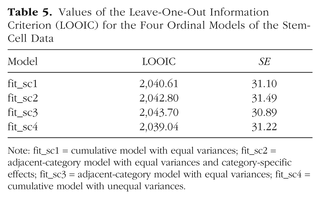
Note: fit_sc1 = cumulative model with equal variances; fit_sc2 = adjacent-category model with equal variances and category-specific effects; fit_sc3 = adjacent-category model with equal variances; fit_sc4 = cumulative model with unequal variances.

Table 6.

Differences Between the Leave-One-Out Information Criteria for the Four Ordinal Models of the Stem-Cell Data

Models	Difference	SE
fit_sc1 vs. fit_sc2	−2.20	4.94
fit_sc1 vs. fit_sc3	−3.10	1.74
fit_sc1 vs. fit_sc4	1.57	5.16
fit_sc2 vs. fit_sc3	−0.90	6.07
fit_sc2 vs. fit_sc4	3.76	1.52
fit_sc3 vs. fit_sc4	4.66	6.34

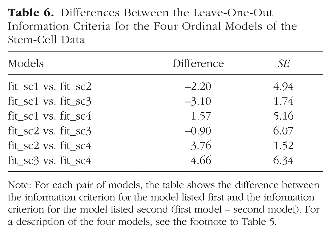
Note: For each pair of models, the table shows the difference between the information criterion for the model listed first and the information criterion for the model listed second (first model – second model). For a description of the four models, see the footnote to Table 5.

In the context of model selection, an LOOIC difference greater than twice its corresponding standard error can be interpreted as suggesting that the model with the lower LOOIC value fits the data substantially better, at least when the number of observations is large enough.⁷ Although the LOOIC differences between the models are not very large, the equal- and unequal-variances cumulative models have somewhat better LOOIC values than the others, and so they might be preferred over the adjacent-category models. However, model selection—based on any metric, be it a p value, Bayes factor, or information criterion—is a controversial and complex topic, and therefore, we suggest replacing hard cutoff values with context-dependent and theory-driven reasoning. For the current example, we favor the unequal-variances cumulative model not only because of its goodness of fit (according to the LOOIC), but also because it is parsimonious and theoretically best justified.

Multiple Likert items

Although they are outside the scope of this Tutorial, we wish to briefly discuss modeling strategies for data with multiple items per person. The extension is straightforward and can be achieved with hierarchical (multilevel) modeling.

In the stem-cell example, we have data for only one item per person. However, in many studies, the participants provide responses to multiple items. In such cases, one can fit a multilevel ordinal model that takes the items and participants into account, incorporating all information in the data into the model while controlling for dependencies between ratings from the same person and between ratings of the same item. For this purpose, the data need to be in long format, such that each row gives a single rating and the columns show the values of ratings and identifiers for the participants and items. If opinion about funding stem-cell research had been measured with multiple items, we might call the identifier columns person and item, respectively. Then, we could write the model formula as follows:

rating ~ 1 + belief + (1|person) + (1|item)

The notation (1|<group>) (e.g., (1|person) or (1|item)) implies that the intercept (1) varies over the levels of the grouping factor (<group>). Ordinal models have multiple intercepts (recall that intercepts are called thresholds in ordinal models), and (1|<group>) allows these thresholds to vary by the same amount across levels of the grouping factor. To model threshold-specific variances, we would write (cs(1)|<group>). For instance, if we want all thresholds to vary differently across items so that each item receives its own set of thresholds, we could add (cs(1)|item) to the model formula.

Summary

In summary, we have illustrated the use of cumulative models (with and without unequal variances) and adjacent-category models (with and without category-specific effects) in the context of a Likert-item response variable. We have illustrated how to fit these four models to data using concise R syntax, enabled by the brm() function, and how to summarize, interpret, and visualize the model’s estimated parameters. Paired with effective visualization (see Fig. 2), the models’ results are readily interpretable and rich in information because of their fully Bayesian estimation. For the data set we used to illustrate the models, we found that category-specific effects did not meaningfully improve model fit, and that the cumulative models were a better fit than the adjacent-category models. Further, there was a small improvement in model fit in the unequal-variances cumulative model relative to the equal-variances cumulative model.

Years until divorce

In our second example, we analyze the marriage data set introduced earlier. We wish to predict the duration (in years) of first marriage (coded as years), which either ends by divorce or continues beyond the time of the survey. These data can be understood as discrete time-to-event data, with the event of interest being divorce. As predictors, we use the participants’ age at marriage (coded as age) and whether the couple was already living together before marriage (coded as together).

Marriage duration can be thought of as a sequential process: Each year, a marriage may continue or end by divorce, but the latter can happen only if it did not happen before. These data clearly call for use of a sequential model to predict the time until divorce (i.e., the time until marriage stops; for alternative formulations, see Appendix A). Further, we assume an extreme-value distribution (corresponding to the cloglog link in brms; see Appendix A for a visualization) for the latent variables ${\tilde{Y}}_{k}$ , because such a distribution is the most common choice in discrete time-to-event models. These data can also be modeled using a cumulative model with a specific latent distribution, such as an extreme-value or Weibull distribution, but for the purpose of this Tutorial, we focus on a sequential model.

In this section, we consider only divorced women in order to illustrate the main ideas of a sequential model as fitted in brms. As noted earlier, we discuss inclusion of nondivorced women (i.e., censored data) in Appendix B. The model including the data of divorced women only is estimated with the following code:

prior_ma <- prior(normal(0, 5), class = ‘b’) +

prior(normal(0, 5), class = ‘Intercept’)

fit_ma1 <- brm(

years ~ 1 + age + together,

data = subset(marriage, divorced),

family = sratio(‘cloglog’),

prior = prior_ma

)

We use a weakly informative normal (0, 5) prior⁸ for all regression coefficients to improve model convergence and to illustrate how to specify prior distributions with brms. Trying to fit this model in a frequentist framework would likely lead to serious convergence issues that would be hard to resolve without the ability to specify priors.

After initially fitting this model, we displayed a summary of the results by using the following code: summary(fit_ma1). We found that women who married later appeared to have shorter marriages (b = −0.04, 95% CI = [−0.07, −0.02]; 95% CI excludes zero), but living together before marriage appeared to be unrelated to years of marriage (b = 0.01, 95% CI = [−0.15, 0.18]). As described earlier, these regression coefficients are defined on the scale of the latent variables ${\tilde{Y}}_{k}$ , which we assumed to be extreme-value distributed. Admittedly, the scale of these coefficients is hard to interpret: The size of the effect of age at marriage, b = −0.04, is not immediately obvious.

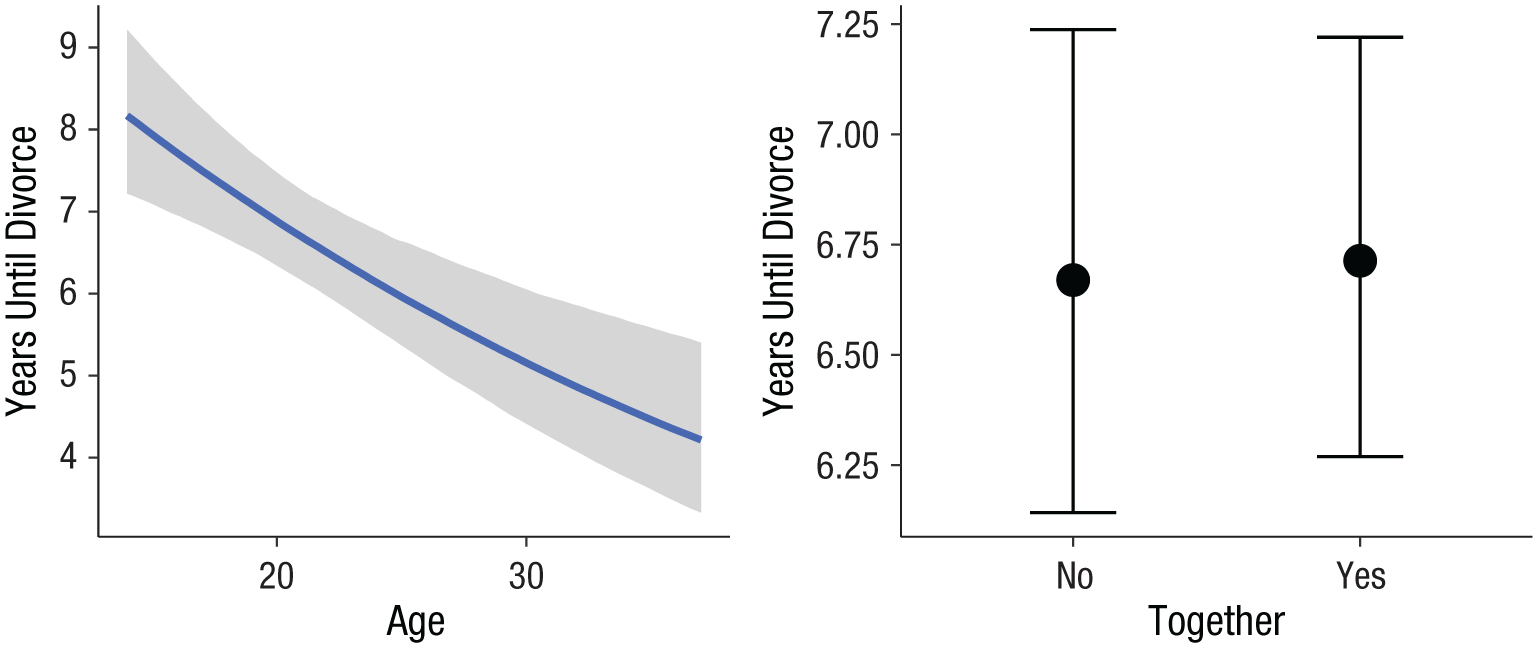
For this reason, we recommend always plotting the results, for instance, with marginal_effects(fit_ma1). In this case, years of marriage has a natural metric interpretation. As shown in the left panel of Figure 3, between the minimum and maximum age at marriage (12 and 43 years, respectively), the model predicts a 3.95-year difference in the time until divorce. In contrast, according to this model, it appears to make little difference whether a couple was living together before marriage (see the right panel of Fig. 3).

Fig. 3.

Marginal effects of a woman’s age at marriage (left) and living together before marriage (right) on the number of years of marriage until divorce, with censored data excluded (data from Centers for Disease Control and Prevention, n.d.). The shaded area in the left panel represents the 95% credible intervals around the estimates.

However, this model omits an important detail in the data: We included only those women who actually got divorced during the study, and excluded those who were still married at the end of the study. In the context of time-to-event analysis, this is called (right) censoring, because divorce might happen later on in time. Both excluding nondivorced women altogether (as we did in the preceding analysis) and falsely treating them as being divorced right at the end of the study may lead to bias of unknown direction and magnitude in the results.

For these reasons, it is important to find a way to incorporate censored data into the model. In the standard version of the sequential model, each observation must have an associated outcome category. However, for censored data, the outcome category was unobserved. Expanding the standard sequential model to include such data requires a little bit of extra work, to which we turn in Appendix B.

Conclusion

In this Tutorial, we have introduced three important classes of ordinal models: cumulative, sequential, and adjacent-category models. We have applied these models to real-world data sets that come from different psychological fields and that can answer different research questions. The models are formally derived from their underlying assumptions in Appendix A, but we do not demonstrate (e.g., via simulations) that using ordinal models for ordinal data is superior to other approaches, such as linear regression, because this topic has already been sufficiently covered elsewhere (Liddell & Kruschke, 2018). Nevertheless, we briefly discuss some possible objections to using ordinal models and provide counterarguments.

Objections and counterarguments

Although we have highlighted the theoretical justification, and practical ease, of applying ordinal models to ordinal data, some readers might still object to using these models. For example, one possible objection is that the results of ordinal models are more difficult to interpret and communicate than the results of corresponding linear regression models. However, the main complexity of ordinal models, relative to linear regression models, is in the threshold parameters, which (like intercept parameters in linear regression) are rarely the main target of inference. Usually, researchers are more interested in the predictors, and the predictors in ordinal models can be interpreted in the same way as ordinary predictors in linear regression models (though they are on the latent metric scale). Furthermore, the helper functions in brms make it easy to calculate (see ?fitted.brmsfit) and visualize (see ?marginal_effects.brmsfit) a model’s fitted values (i.e., the predicted proportion of each response category for a given set of predictor values).

Another possible objection is that sometimes one’s substantial conclusions do not strongly depend on whether an ordinal or a linear regression model was used. We wish to point out, though, that even though the actionable conclusions may be similar, a linear model will have a lower predictive utility by virtue of assuming a theoretically incorrect outcome distribution. Perhaps more important is the fact that using linear models for ordinal data can lead to effect-size estimates that are distorted in size or certainty, and this problem is not solved by averaging data for multiple ordinal items (Liddell & Kruschke, 2018).

Software options

We have advocated and illustrated the implementation of ordinal models using the brms package in the R statistical computing environment. The main reason for our choice of these software options is that they are completely free and open source. Therefore, they are available to anyone, without any licensing fees. In addition, many computational and statistical procedures are implemented in R before they are available in other (commercial) software packages. Further, we believe that the wide variety of models that can be computed through the concise and consistent syntax of brms is beneficial to any modeling endeavor (Bürkner, 2017, 2018).

Nevertheless, users may wish to implement ordinal models within their preferred statistical packages. Explaining how to conduct ordinal regressions using other software is outside the scope of this Tutorial. Useful references include Heck, Thomas, and Tabata (2013) for IBM SPSS; Bender and Benner (2000) for SAS and S-Plus; and Long, Long, and Freese (2006) for Stata.

Choosing between ordinal models

Equipped with the knowledge about the three classes of ordinal models, researchers might still find it difficult to decide which type of model best fits their research question and data. It is impossible to describe in advance which class would best fit each situation, but here we briefly describe some useful rules of thumb for deciding among the models we have discussed.

From a theoretical perspective, if the response under study can be understood as the categorization of a latent continuous construct, we recommend using a cumulative model. The categorization interpretation is natural for many Likert-item data sets, in which ordered verbal (or numerical) labels are used to obtain discrete responses about a continuous psychological variable. Cumulative models are also computationally less intensive than the other types of models, and therefore faster to estimate. If unequal variances are theoretically possible—and they usually are—we recommend incorporating them into the model; ignoring them may lead to increased false alarm rates and inaccurate parameter estimates (Liddell & Kruschke, 2018). Further, we think that (differences in) variances, although often overlooked, can themselves be theoretically interesting and therefore should be modeled.

If the response under study can be understood as the result of a sequential process, such that a higher response category is possible only after all lower categories are achieved, we recommend using a sequential model. Sequential models are therefore especially useful, for example, for discrete time-to-event data. However, deciding between a categorization and a sequential process may not always be straightforward; in ambiguous situations, estimating both types of models may be a reasonable strategy.

If category-specific effects are of interest, we recommend using a sequential or adjacent-category model. It is useful to model category-specific effects when there is reason to expect that a predictor might affect the response variable differently at different levels of the response variable. Finally, we suggest that if one wishes to model ordinal responses, it is important to use an ordinal model of any type instead of falsely assuming metric or nominal responses.

Supplemental Material

BurknerOpenPracticesDisclosure – Supplemental material for Ordinal Regression Models in Psychology: A Tutorial

Supplemental material, BurknerOpenPracticesDisclosure for Ordinal Regression Models in Psychology: A Tutorial by Paul-Christian Bürkner and Matti Vuorre in Advances in Methods and Practices in Psychological Science

Footnotes

Appendix A: Derivations of the Three Classes of Ordinal Models

In this appendix, we derive and discuss in more detail the classes of ordinal models illustrated in the main text. Throughout, we assume that the data consist of a total of N values of the ordinal response variable Y with K + 1 categories from 1 to K + 1.

Appendix B: Modeling the Number of Years Until Divorce

In this appendix, we continue with the discussion of using a sequential model to predict the number of years of marriage until divorce. In particular, we show how to incorporate censored data into the sequential model we described earlier for analyzing the marriage-duration data from the U.S. National Survey of Family Growth (Centers for Disease Control and Prevention, n.d.). This extension is necessary because—quite fortunately—not all marriages ended with divorce at the end of the study’s observation period.

In the field of time-to-event analysis, the hazard rate plays a crucial role (Cox, 1972). For discrete time-to-event data, the hazard rate at time t, h(t), is simply the probability that the event occurs at time t given that the event did not occur up through time t – 1. In our notation, the hazard rate at time t can be written as

(B1)

h (t) = F (τ_{t} - η) .

Comparing this with Equation A15, we see that the stopping sequential model is simply the product of h(t) and 1 – h(t) terms for varying values of t. Each of these terms defines the event probability of a Bernoulli variable (0 = still married beyond time t; 1 = divorced at time t), so the sequential model can be understood as a sequence of conditionally independent Bernoulli trials. Accordingly, we can equivalently write the sequential model in terms of binary regression¹⁰ by expanding each of the outcome variables into a sequence of 0s and 1s.¹¹ More precisely, for each couple, we create a single row for each year of marriage, entering the outcome variable as 1 if the couple divorced in that year and as 0 otherwise. The expanded data are exemplified in Table B1.

In the expanded data set, discrete_time indicates the length of the marriage (in years) for each row of the data. It is treated as a factor so that, when it is included in a model formula in brms, its coefficients will represent the threshold parameters. This can be done in at least two ways. First, we could write … ~ 0 + discrete_time + … , in which case the coefficients can immediately be interpreted as thresholds. Second, we could write … ~ 1 + discrete_time + … , so that the intercept is the first threshold, and the $K - 1$ coefficients of discrete_time represent differences between the respective other thresholds and the first threshold (dummy coding). Note that these representations are equivalent in the sense that we can transform one into the other. However, the second option usually leads to improved sampling, because it allows brms to do some internal optimization. We are now ready to fit a binary regression model to the expanded data set, which we do with the following code:

fit_ma2 <- brm(

divorced ~ 1 + discrete_time + age + together,

data = marriage_long,

family = bernoulli("cloglog"),

prior = prior_ma,

inits = 0

)

The estimated coefficients of this model are summarized in Table B2. We did not include the threshold estimates in order to keep the table readable. Figure B1 illustrates the output of the model, showing marginal model predictions for the probability of divorce in the 7th year of marriage. Because this figure shows the probability of divorce and Figure 3 shows the duration of marriage, the two figures would show opposite patterns if including the censored data did not have a dramatic effect. To the contrary, age at marriage has the same sign in the two models, which means they lead to opposite conclusions: Whereas the model without the censored data predicts longer-lasting marriages (lower probability of divorce) for women marrying at younger ages, the model with the censored data predicts a lower probability of divorce for women marrying at older ages. These results are plausible insofar as censoring was confounded with age at marriage: Women who married at older ages were more likely to still be married at the time of the survey. Moreover, in contrast to the model without the censored data, the model including those data reveals that couples who lived together before marriage had a considerably lower probability of getting divorced than couples who did not live together. These results underline the importance of correctly including censored data in (discrete) time-to-event models, and we have demonstrated how to do this in the framework of the ordinal sequential model.

Finally, because this survey on marriage duration took place at one time and asked retrospective questions, we did not have reliable information on any time-varying predictors, but we can easily think of some potential ones. For instance, the probability of divorce may change over the duration of marriage as a couple’s socioeconomic status changes. Such time-varying predictors cannot be modeled in the standard sequential model, because all information about a single marriage process has to be stored within the same row in the data set. Fortunately, time-varying predictors can easily be added to the expanded data set shown in Table B2 and then treated in the same way as other predictors in the binary regression model.

Action Editor

Pamela Davis-Kean served as action editor for this article.

Author Contributions

P.-C. Bürkner generated the idea for the manuscript and wrote the first draft of the theoretical part of the manuscript. The two authors jointly wrote the first draft of the practical part of the manuscript. Both authors critically edited the entire draft and approved the final submitted version of the manuscript.

ORCID iDs

Paul-Christian Bürkner

Matti Vuorre

Declaration of Conflicting Interests

The author(s) declared that there were no conflicts of interest with respect to the authorship or the publication of this article.

Open Practices

All data and materials have been made publicly available via the Open Science Framework and can be accessed at https://osf.io/cu8jv/. The complete Open Practices Disclosure for this article can be found at http://journals.sagepub.com/doi/suppl/10.1177/2515245918823199. This article has received badges for Open Data and Open Materials. More information about the Open Practices badges can be found at .

Notes

References

Adams

R. J.

M. L.

Wilson

(2012). The Rasch rating model and the disordered threshold controversy. Educational and Psychological Measurement, 72, 547–573. doi:10.1177/0013164411432166

Agresti

(1984). Analysis of ordinal categorical data. Chichester, England: John Wiley & Sons.

Agresti

(2010). Analysis of ordinal categorical data (2nd ed.). Chichester, England: John Wiley & Sons. doi:10.1002/9780470594001

Akaike

(1998). Information theory and an extension of the maximum likelihood principle. In Parzen

Tanabe

Kitagawa

(Eds.), Selected papers of Hirotugu Akaike (pp. 199–213). New York, NY: Springer.

Ananth

C. V.

Kleinbaum

D. G.

(1997). Regression models for ordinal responses: A review of methods and applications. International Journal of Epidemiology, 26, 1323–1333.

Andersen

E. B.

(1973). Conditional inference for multiple-choice questionnaires. British Journal of Mathematical and Statistical Psychology, 26, 31–44. doi:10.1111/j.2044-8317.1973.tb00504.x

Andersen

E. B.

(1977). Sufficient statistics and latent trait models. Psychometrika, 42, 69–81.

Andrich

(1978a). Application of a psychometric rating model to ordered categories which are scored with successive integers. Applied Psychological Measurement, 2, 581–594.

Andrich

(1978b). A rating formulation for ordered response categories. Psychometrika, 43, 561–573. doi:10.1007/BF02293814

10.

Andrich

(2005). The Rasch model explained. In Maclean

Watanabe

Baker

Boediono Cheng

Y. C.

Duncan

. . .Hungi

(Eds.), Applied Rasch measurement: A book of exemplars (pp. 27–59). Dordrecht, The Netherlands: Springer. doi:10.1007/1-4020-3076-2_3

11.

Bender

Benner

(2000). Calculating ordinal regression models in SAS and S-Plus. Biometrical Journal, 42, 677–699. doi:10.1002/1521-4036(200010)42:6<677::AID-BIMJ677>3.0.CO;2-O

12.

Betancourt

(2017). A conceptual introduction to Hamiltonian Monte Carlo. arXiv. Retrieved from https://arxiv.org/abs/1701.02434

13.

Bürkner

P.-C.

(2017). brms: An R package for Bayesian multilevel models using Stan. Journal of Statistical Software, 80(1). doi:10.18637/jss.v080.i01

14.

Bürkner

P.-C.

(2018). Advanced Bayesian multilevel modeling with the R package brms. The R Journal, 10, 395–411.

15.

Carpenter

Gelman

Hoffman

M. D.

Lee

Goodrich

Betancourt

. . . Riddell

(2017). Stan: A probabilistic programming language. Journal of Statistical Software, 76(1). doi:10.18637/jss.v076.i01

16.

Centers for Disease Control and Prevention. (n.d.). 2013-2015 NSFG: Public use data files, codebooks, and documentation. Retrieved from https://www.cdc.gov/nchs/nsfg/nsfg_2013_2015_puf.htm

17.

Cox

D. R.

(1972). Regression models and life-tables [Target article and discussion]. Journal of the Royal Statistical Society, Series B (Methodological), 34, 187–220.

18.

Eager

Roy

(2017). Mixed effects models are sometimes terrible. arXiv. Retrieved from http://arxiv.org/abs/ 1701.04858

19.

Fienberg

S. E.

(2007). The analysis of cross-classified categorical data. New York, NY: Springer Science & Business Media. (Original work published 1980)

20.

Fischer

G. H.

(1995). The derivation of polytomous Rasch models. In Fischer

G. H.

Molenaar

I. W.

(Eds.), Rasch models (pp. 293–305). New York, NY: Springer. doi:10.1007/978-1-4612-4230-7_16

21.

Gelman

Carlin

J. B.

Stern

H. S.

Dunson

D. B.

Vehtari

Rubin

D. B.

(2013). Bayesian data analysis (3rd ed.). Boca Raton, FL: CRC Press.

22.

Gibbons

J. D.

Chakraborti

(2011). Nonparametric statistical inference. In Lovric

(Ed.), International encyclopedia of statistical science (pp. 977–979). Berlin, Germany: Springer.

23.

Guisan

Harrell

F. E.

(2000). Ordinal response regression models in ecology. Journal of Vegetation Science, 11, 617–626.

24.

Heck

R. H.

Thomas

Tabata

(2013). Multilevel modeling of categorical outcomes using IBM SPSS. New York, NY: Routledge.

25.

Hoekstra

Morey

R. D.

Rouder

J. N.

Wagenmakers

E.-J.

(2014). Robust misinterpretation of confidence intervals. Psychonomic Bulletin & Review, 21, 1157–1164. doi:10.3758/s13423-013-0572-3

26.

Kruschke

J. K.

(2014). Doing Bayesian data analysis: A tutorial introduction with R (2nd ed.). Burlington, MA: Academic Press.

27.

Kruschke

J. K.

Liddell

T. M.

(2018a). Bayesian data analysis for newcomers. Psychonomic Bulletin & Review, 25, 155–177.

28.

Kruschke

J. K.

Liddell

T. M.

(2018b). The Bayesian New Statistics: Hypothesis testing, estimation, meta-analysis, and power analysis from a Bayesian perspective. Psychonomic Bulletin & Review, 25, 178–206.

29.

Läärä

Matthews

(1985). The equivalence of two models for ordinal data. Biometrika, 72, 206–207.

30.

Liddell

Kruschke

J. K.

(2018). Analyzing ordinal data with metric models: What could possibly go wrong? Journal of Experimental Social Psychology, 79, 328–348.

31.

Long

S. J.

Long

J. S.

Freese

(2006). Regression models for categorical dependent variables using Stata (2nd ed.). College Station, TX: Stata Press.

32.

Masters

G. N.

(1982). A Rasch model for partial credit scoring. Psychometrika, 47, 149–174. doi:10.1007/BF02296272

33.

McCullagh

(1980). Regression models for ordinal data. Journal of the Royal Statistical Society, Series B (Methodological), 42, 109–142.

34.

McElreath

(2016). Statistical rethinking: A Bayesian course with examples in R and Stan. Boca Raton, FL: CRC Press.

35.

Mellenbergh

G. J.

(1995). Conceptual notes on models for discrete polytomous item responses. Applied Psychological Measurement, 19, 91–100.

36.

Molenaar

(1983). Item steps (Heymans Bulletin HB-83-630-EX). Groningen, The Netherlands: University of Groningen, Vakgroep Statistiek En Meettheorie.

37.

Morey

R. D.

Hoekstra

Rouder

J. N.

Lee

M. D.

Wagenmakers

E.-J.

(2016). The fallacy of placing confidence in confidence intervals. Psychonomic Bulletin & Review, 23, 103–123.

38.

OECD. (2017). PISA 2015: Technical report. Retrieved from http://www.oecd.org/pisa/data/2015-technical-report/

39.

Peterson

Harrell

F. E.

Jr. (1990). Partial proportional odds models for ordinal response variables. Journal of the Royal Statistical Society, Series C (Applied Statistics), 39, 205–217.

40.

Rasch

(1961). On general laws and the meaning of measurement in psychology. In Neyman

(Ed.), Proceedings of the Fourth Berkeley Symposium on Mathematical Statistics and Probability: Vol. IV. Biology and problems of health (pp. 321–333). Berkeley: University of California Press.

41.

R Core Team. (2017). R: A language and environment for statistical computing. Retrieved from https://www.R-project.org/

42.

Samejima

(1969). Estimation of latent ability using a response pattern of graded scores. Psychometrika, 34(Suppl.).

43.

Samejima

(1995). Acceleration model in the heterogeneous case of the general graded response model. Psychometrika, 60(4), 549–572.

44.

Samejima

(1997). Graded response model. In van der Linden

Hambleton

R. K.

(Eds.), Handbook of modern item response theory (pp. 85–100). New York, NY: Springer.

45.

Stevens

S. S.

(1946). On the theory of scales of measurement. Science, 103, 677–680. doi:10.1126/science.103.2684.677

46.

Teachman

(2011). Modeling repeatable events using discrete-time data: Predicting marital dissolution. Journal of Marriage and Family, 73, 525–540.

47.

Tutz

(1990). Sequential item response models with an ordered response. British Journal of Mathematical and Statistical Psychology, 43, 39–55. doi:10.1111/j.2044-8317.1990.tb00925.x

48.

Tutz

(1997). Sequential models for ordered responses. In van der Linden

Hambleton

R. K.

(Eds.), Handbook of modern item response theory (pp. 139–152). New York, NY: Springer.

49.

Tutz

(2000). Die Analyse Kategorialer Daten: Anwendungsorientierte Einführung in Logit-Modellierung und Kategoriale Regression [Analysis of categorical data: An application oriented introduction to logit modeling and categorical regression]. Oldenbourg, Germany: Oldenbourg Verlag.

50.

Van Der Ark

L. A.

(2001). Relationships and properties of polytomous item response theory models. Applied Psychological Measurement, 25, 273–282. doi:10.1177/01466210122032073

51.

van der Linden

Hambleton

R. K.

(Eds.). (1997). Handbook of modern item response theory. New York, NY: Springer.

52.

van Ravenzwaaij

Cassey

Brown

S. D.

(2018). A simple introduction to Markov Chain Monte–Carlo sampling. Psychonomic Bulletin & Review, 25, 143–154. doi:10.3758/s13423-016-1015-8

53.

Vehtari

Gelman

Gabry

(2017). Practical Bayesian model evaluation using leave-one-out cross-validation and WAIC. Statistics and Computing, 27, 1413–1432.

54.

Verhelst

N. D.

Glas

De Vries

(1997). A steps model to analyze partial credit. In van der Linden

Hambleton

R. K.

(Eds.), Handbook of modern item response theory (pp. 123–138). New York, NY: Springer.

55.

Vuorre

(2016, December 5). Introduction to data analysis using R. JEPS Bulletin. Retrieved from http://blog.efpsa.org/2016/12/05/introduction-to-data-analysis-using-r/

56.

Walker

S. H.

Duncan

D. B.

(1967). Estimation of the probability of an event as a function of several independent variables. Biometrika, 54, 167–179. doi:10.2307/2333860

57.

Watanabe

(2010). Asymptotic equivalence of Bayes cross validation and widely applicable information criterion in singular learning theory. Journal of Machine Learning Research, 11, 3571–3594.

58.

Wickham

Grolemund

(2016). R for data science. Retrieved from http://r4ds.had.co.nz/

59.

Wilson

(1992). The ordered partition model: An extension of the partial credit model. Applied Psychological Measurement, 16, 309–325. doi:10.1177/014662169201600401

60.

Wilson

Adams

R. J.

(1993). Marginal maximum likelihood estimation for the ordered partition model. Journal of Educational and Behavioral Statistics, 18, 69–90. doi:10.2307/1165183

Supplementary Material

Please find the following supplemental material available below.

For Open Access articles published under a Creative Commons License, all supplemental material carries the same license as the article it is associated with.

For non-Open Access articles published, all supplemental material carries a non-exclusive license, and permission requests for re-use of supplemental material or any part of supplemental material shall be sent directly to the copyright owner as specified in the copyright notice associated with the article.

0.00 MB

0.64 MB