Sage Journals: Discover world-class research

Abstract

New pipelines are required to automate the quantitation of emerging high-throughput electrophoretic (EP) assessment of DNA damage, or proteoform expression in single cells. EP cytometry consists of thousands of Western blots performed on a microscope slide-sized gel microwell array for single cells. Thus, EP cytometry images pose an analysis challenge that blends requirements for accurate and reproducible analysis encountered for both standard Western blots and protein microarrays. Here, we introduce the Summit algorithm to automate array segmentation, peak background subtraction, and Gaussian fitting for EP cytometry. The data structure storage of parameters allows users to perform quality control on identically processed data, yielding a ~6.5% difference in coefficient of quartile variation (CQV) of protein peak area under the curve (AUC) distributions measured by four users. Further, inspired by investigations of background subtraction methods to reduce technical variation in protein microarray measurements, we aimed to understand the trade-offs between EP cytometry analysis throughput and variation. We found an 11%–50% increase in protein peaks that passed quality control with a subtraction method similar to microarray “average on-boundary” versus an axial subtraction method. The background subtraction method only mildly influences AUC CQV, which varies between 1% and 4.5%. Finally, we determined that the narrow confidence interval for peak location and peak width parameters from Gaussian fitting yield minimal uncertainty in protein sizing. The AUC CQV differed by only ~1%–2% when summed over the peak width bounds versus the 95% peak width confidence interval. We expect Summit to be broadly applicable to other arrayed EP separations, or traditional Western blot analysis.

Keywords

data analysis (informatics and software)microfluidics (microtechnology)Western blot high-throughput arrays

Introduction

Electrophoretic (EP) separations provide critical information regarding the physicochemical properties and abundance of a given protein or proteoform.¹ Examples of physicochemical properties that separations can quantify include the protein molecular mass (as in sodium dodecyl sulfate–polyacrylamide gel electrophoresis [SDS-PAGE]²), isoelectric point (determined by isoelectric focusing³), or both (via 2D electrophoresis⁴). Such separations are performed in a variety of formats, including slab gels, microchannels,^5,6 and capillaries,^7–9 each with specially designed analyses to quantify properties of the electropherogram. However, some analyses of EP separations still require substantial manual processing, such as the nonstandardized and poorly documented practices employed for densitometry of Western blotting.¹⁰ Western blotting utilizes a size-based EP separation followed by a transfer of the separated analytes to a membrane (blotting) on which proteins are detected with fluorescent or chemiluminescent antibodies. Currently, it is still typical for the user to manually outline regions of the image to quantify (e.g., selecting the protein bands) using commercially available software sold with Western blot imagers. In a random survey of 100 publications from PubMed that utilized densitometry for Western blotting quantitation, only one paper provided sufficient details for the analysis to be reproduced¹⁰ (e.g., how bands were selected, whether peak integrals or heights were used for quantification, and type of intensity profile background subtraction).

Manual processing becomes impractical for high-throughput EP separations. Our group and others have introduced high-throughput EP separations with up to hundreds to thousands of separations performed in parallel across an array,^11–16 or with 1300 separations in series in a capillary.¹⁷ Applications of arrayed separations include assessing cell-to-cell heterogeneity in DNA damage via single-cell comet assays,^18,19 and quantifying proteoforms responsible for cancer drug resistance in breast cancer with EP cytometry.²⁰

EP cytometry performs thousands of single-cell protein separations in a device patterned on a standard microscope slide, and protein peaks are detected with fluorescent antibodies. We previously developed quantitative algorithms for EP cytometry to determine protein expression levels by area under the curve (AUC) analysis.^13,21 However, the previous algorithms were cumbersome (with 10–20+ functions) and did not include features that would enable reproducible analysis.

Image processing of microscopy data faces similar challenges in accessibility, scale, and reproducibility. To aid in the accessibility of the analysis, image processing tools such as CellProfiler²² and Ilastik²³ have introduced graphical user interfaces (GUIs) that guide the user through the analysis. Once the image processing pipeline is established, the user can then apply the same analysis across large data sets via a batch processing mode. Further, toward improving reproducibility, CellProfiler and Ilastik allow the user to save the analysis pipeline to a file that contains all of the relevant parameters. Starfish,²⁴ a toolkit for processing in situ transcriptomics data, approaches reproducible analysis by storing the results in data structures that automatically record the information required to reproduce the analysis (e.g., parameters used, versions of the software dependencies). However, processing of microscopy images of cells differs from the analysis needed for EP separation images, in which protein peak locations along a defined separation axis may be used to size and identify proteoforms. Existing image processing tools can quantify the integrated fluorescence (amount of protein) from segmented images, but are not readily adaptable to identify a separation lane to index protein band locations.

Inspired by advances in image processing toolkits for microscopy data, we introduce Summit for EP cytometry quantitation and assess the impact of specific algorithm design choices on measured single-cell protein and intrauser variation. Functional decomposition was employed to establish the four functions of Summit. The algorithm requires minimal user interaction through the use of GUIs, making it accessible to researchers of all computational backgrounds. Design choices, including data storage in a structure, background subtraction method, and quality control thresholding, are described. Analysis reproducibility is confirmed as differences in protein AUC distributions are not statistically significant when quantified by four different Summit users. When comparing background subtraction methods, we find that mean subtraction (similar to average on-boundary subtraction in 2D electrophoresis) yields 11%–50% more quantifiable single-cell protein peaks compared with the axial subtraction method used in our previous work. Such throughput gains come without substantial increases in variation in measured protein. We find that the appropriate background subtraction method for a given protein can be evaluated by comparing variation in the peak offset after subtraction and the AUC confidence interval with different peak bounds for summation. The guidelines presented here will aid in accurate and reproducible EP cytometry image analysis for various basic research and clinical applications.

Materials and Methods

Reagents

All reagents used are summarized in the Supplemental Information.

Cell Culture

Cell culture conditions are summarized in the Supplemental Information. All cell lines tested negative for mycoplasma and were authenticated by short tandem repeat analysis (Promega, Madison, WI) (see Suppl. Figs. S1–S3 ).

EP Cytometry Separations

EP cytometry was performed as described in detail elsewhere^21,25 and is summarized in the Supplemental Information and Supplemental Table S1 , and EP cytometry images from breast cancer tumor-derived cells are from a previously published work in which EP cytometry conditions were described.²⁰ The example proteins characterized in this work are GFP, GAPDH, HER2, rs6, and p-rs6. GFP and GAPDH are from distinct EP cytometry experiments (different cell types, different images), while HER2, rs6, and p-rs6 are from the same EP cytometry experiment (breast cancer tissue-derived cells, distinct fluorescence channels of the same EP cytometry image). All images are available on Figshare repositories: EP cytometry of tumor 0909 for HER2, rs6, and p-rs6: https://figshare.com/s/fc77c1ca77e6976f3c59; and EP cytometry for GFP, GAPDH, and simulated skewed peak images: https://doi.org/10.6084/m9.figshare.13557482.v1.

Summit was written for MATLAB version 9.1 (2016b; MathWorks, Natick, MA) or higher. MATLAB program file dependencies of Summit include the Image Processing Toolbox (version 9.5 or higher) and the Curve Fitting Toolbox (version 3.5.4 or higher). The complete source code is available on GitHub (https://github.com/herrlabucb/summit), and instructions for installing Summit are provided in the repository readme.

Statistical Analysis

All box plots display the median, with the box edges at the 25th and 75th percentiles and whiskers that extend to the minimum and maximum values. The Mann–Whitney U test, Kruskal–Wallis test, Dunn–S Sidak post hoc comparison test, and linear regression were performed using built-in functions in MATLAB (2019b).

Results

The aim of EP cytometry image processing is to both quantify the protein expression and estimate the molecular mass (when using appropriate sizing standards). We developed the Summit image processing pipeline to be modular by using functional decomposition to discretize the pipeline into four functions. The raw image in Figure 1A contains 1615 individual separation lanes that are processed in the four functions shown in Figure 1B : (1) regions of interest (ROIs) are segmented; (2) a 1D intensity profile is generated and the background subtracted; (3) the intensity profile is fit to a Gaussian curve; and (4) the user inspects the fitted peaks as a final quality control step. From analysis of the protein peak AUC, cell-to-cell heterogeneity in protein expression or correlation between proteins in known cancer signaling networks can be quantified ( Fig. 1C ). Leveraging protein sizing in SDS-PAGE, Gaussian fit-determined peak locations of proteins can identify the mass of proteoforms, such as the truncated HER2 protein species t-erbB2 (~95–115 kDa) that confers trastuzumab resistance in HER2-positive breast cancer^20,26 ( Fig. 1D , E ). In this instance, the pixel intensities for t-erbB2 are summed across the width of the ROI to produce the 1D intensity profile for background subtraction and Gaussian fitting to identify the peak location.

Figure 1.

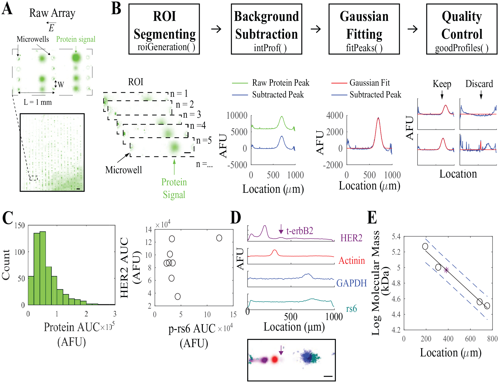
Summit is a semiautomated algorithm that extracts quantitative parameters such as protein peak AUC and peak location from EP cytometry images containing thousands of protein separations. (A) False-colored fluorescence image of an EP cytometry array with detection of GFP from MCF-7 GFP cells (scale bar = 1 mm). The electric field (E) direction is indicated. A subset of the array is shown with two columns and four rows of microwells mostly containing protein signal (except the empty microwell in column 1, row 2). Width between rows (W) = 0.25 mm. (B) Summit workflow with corresponding function names and false-colored fluorescence micrographs (scale bar = 0.1 mm) of GFP protein signal, intensity profiles, Gaussian fits, and quality control. (C) Histogram of GFP peak AUC (from MCF-7 GFP cells) and scatterplot of HER2 versus phospho-s6 AUC (breast cancer tumor; n = 8 cells) as quantified by the algorithm. (D) False-colored fluorescence micrograph and intensity profiles of HER2, actinin, GAPDH, and rs6 protein from breast cancer tumor cell (scale bar = 0.1 mm). Truncated protein isoform t-erbB2 is shown with an arrow. (E) Plot of log-linear regression fitting (black solid line) of known molecular mass versus Gaussian fit-determined peak location of HER2, actinin, GAPDH, and rs6 from D (y = −0.0013x + 5.479; R² = 0.98). The t-erbB2 (purple asterisk) has a mass of 91.4 kDa based on fit. The 95% prediction interval for the fit is shown (blue dashed line).

User interaction is limited to the selection of array boundaries in the ROI segmentation function, the selection of peak boundaries in the curve-fitting function, and the quality control function. There are options to input thresholding parameters to assist with quality control, or the user may choose to manually inspect each separation lane, as described in more detail in the quality control section. Here, the reproducibility and accuracy of quantitation using Summit are explored in detail.

Assessing Analysis Reproducibility

To ensure that the results of an analysis performed with Summit are reproducible, we specified the output of the Summit analysis pipeline to include all parameters necessary to perform the analysis. By selecting a data structure for algorithm output variable storage, variables of different data types can be saved within a single file ( Suppl. Table S2 ) and accessed by the field in the command line. Output variables allow the analysis to be reproduced by another user if they have access to the data structure. In order to achieve analysis reproducibility, parameters for EP cytometry image segmentation to ROIs must be logged and ROIs should be able to be duplicated (either by other users or by the same user analyzing multiple images from the same EP cytometry device).

We leverage the arrayed format of most EP cytometry separation devices in the image segmentation process to generate the ROIs for each separation lane ( Fig. 2 ) using the roiGeneration function. In order to establish array boundaries and align the separation axes with the vertical axis of the image, a GUI first prompts the user to select microwells within a row approximately 10 microwells apart ( Fig. 2A, B ). The necessary angle of rotation to straighten or align the image is calculated from the two points. The rotation is performed with a built-in MATLAB function, imrotate(), which takes inputs of an image and an angle. The function first translates the image centroid to the origin (the upper left corner of the image), and then the image matrix is rotated around the origin by the angle calculated from the dot product of two direction vectors between the two selected microwell coordinates. Following rotation, the matrix is translated back to the original centroid location. After rotation, the user is instructed to select four microwells along the row and column boundaries of the array ( Fig. 2C ). The function informs the user if they have selected incorrect boundaries (e.g., if the coordinate of the “top-most” well of the array is lower than the coordinate of the “bottom-most”). As the gel is attached to a glass slide, image warping does not hinder the use of array boundaries and well spacings to segment the image. The aligned image is next segmented into ROIs based on the user input well-to-well spacing ( Fig. 2D ). The length (L) and width (W) of each lane set the ROI dimensions. The ROIs are then stored in the data structure as an L × W × N array, where N is the number of separation lanes. As an optional input variable of roiGeneration(), the user may provide a data structure with parameters such as the user-selected array boundaries, and angle of rotation, to apply the same ROIs to another EP cytometry image.

Figure 2.

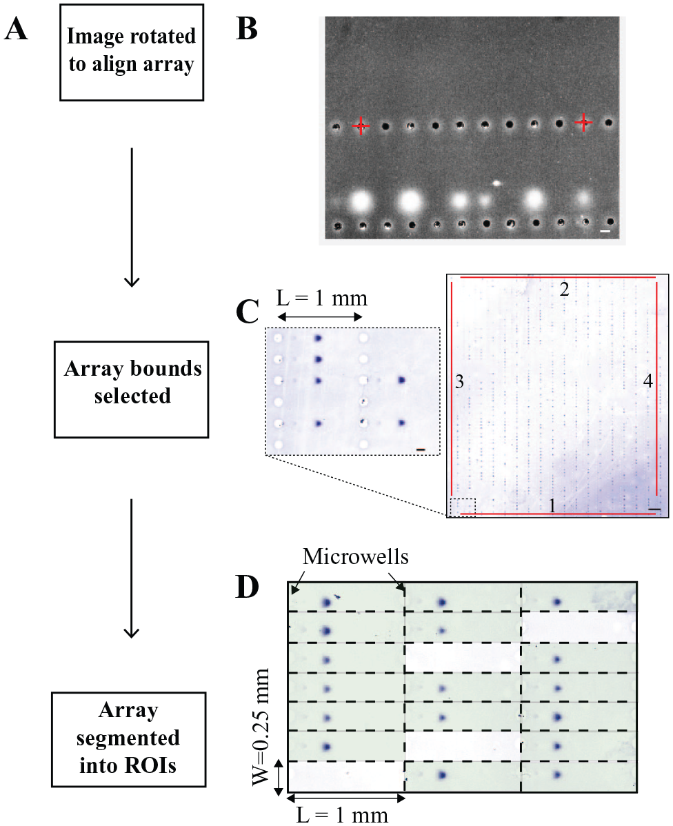
The EP cytometry image is rotated to align the array before segmentation into thousands of individual ROIs. (A) Process workflow. (B) False-colored fluorescence micrograph showing two rows of microwells with user selection of two microwells indicated with red plus signs for image alignment with the MATLAB function imrotate(). Scale bar is 0.1 mm. (C) False-colored fluorescence micrograph with example of user-selected array boundaries (red lines indicating rows or columns of microwells at the edges of the array). The numbers indicate the required order of selection. Scale bar = 1 mm. Inset is a false-colored fluorescence micrograph in the region of the first array bound (scale bar = 0.1 mm). (D) False-colored fluorescence micrograph of a subset of the array segmented into ROIs with a length (L) and width (W) input by the user. ROIs with protein signal from cells are shaded green.

When four users, users 1–4 (including two developers, users 1–2), independently performed EP cytometry analysis with Summit (using identical ROIs), they did not find substantial differences between the measured protein AUC distributions. We utilize Gaussian curve fitting to determine protein expression via AUC analysis.¹⁰ The Gaussian fit function, f(x), employed is

f (x) = a e^{- {(\frac{x - μ}{b})}^{2}}

(1)

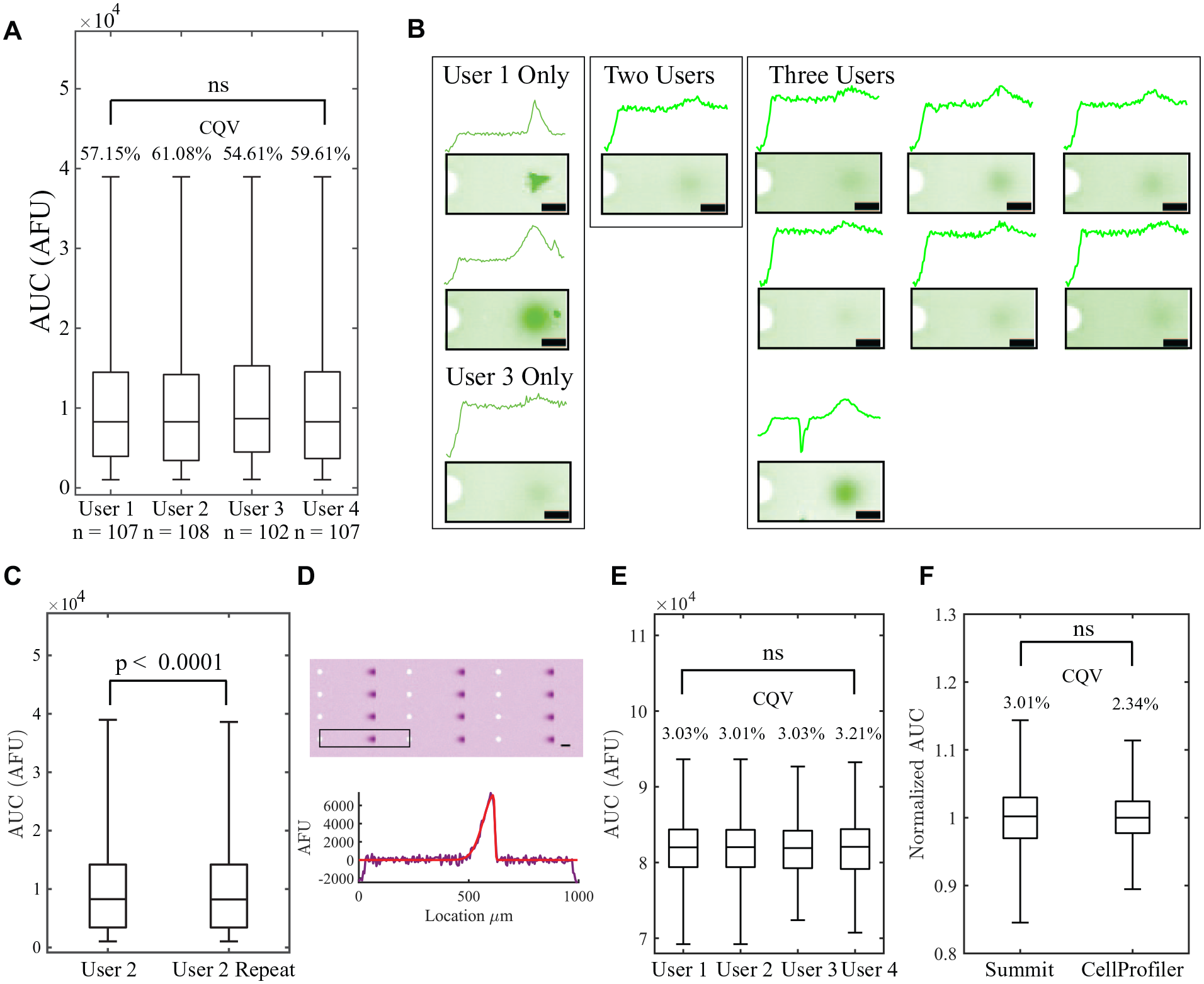
where a is the amplitude, μ is the peak center, and b is the peak width. The protein peaks assume a Gaussian distribution owing to protein diffusion during the EP separation.²⁷ The AUC may be determined by summing over μ ± 2σ, where $σ = \frac{b}{\sqrt{2}} .$ We choose the summation bounds that correspond with the 95% confidence interval for a Gaussian distribution²⁸). As shown in Figure 3A , we cannot reject the null hypothesis, and thus the AUC distributions quantified by the four users can be considered as drawn from a single distribution (Kruskal–Wallis p > 0.05).

Figure 3.

Analysis automation yields insignificant interuser and intrauser variation in quantified protein signal for EP cytometry images collected experimentally and generated by simulation. (A) Box plot of AUC from EP cytometry images of native turbo GFP from U251-GFP cells quantified by four algorithm users, users 1–4 (users 1 and 2 are the developers). Kruskal–Wallis p = 0.95 (and p > 0.99 for Dunn–Sidak correction for multiple comparisons). The number of ROIs that passed quality control (n) and the CQV are shown. (B) False-colored fluorescence micrographs and intensity profiles for every ROI that users 1–4 did not agree upon. Three peak images passed quality control from only one user out of four (i.e., “User 1 Only” and “User 3 Only”). One peak image passed quality control from two out of four users (“Two Users”), and seven passed quality control from combinations of three out of four users (“Three Users”). Scale bar = 100 μm. (C) Box plot of AUC from the GFP image upon repeat analysis by user 2, days after initial analysis. Wilcoxon signed-rank test p < 0.0001 for 108 out of the 112 peaks that passed quality control on initial and repeat analyses (with 62 tied values). (D) False-colored fluorescence micrograph of simulated skewed Gaussian peaks and representative intensity profile for the ROI outlined in black. The skewed Gaussian fit is shown in red (R² = 0.98). Scale bar = 100 μm. (E) Box plot of AUC from the simulated skew peak image analyzed by users 1–4. Kruskal–Wallis p = 0.98 (and p > 0.99 for Dunn–Sidak correction for multiple comparisons). (F) Box plot of AUC normalized to the mean for the simulated skew peak image analyzed by Summit and CellProfiler. Mann–Whitney p = 0.82.

To assess differences between the four users in variation in AUC (which will not be normally distributed²⁹), we quantified the CQV, which is recommended over the coefficient of variation for skewed distributions:³⁰

C Q V = \frac{Q_{3} - Q_{1}}{Q_{3} + Q_{1}}

(2)

where Q₃ and Q₁ are the third and first quartile of the distribution. The CQVs only differ by ~6.5% between the distributions measured by the four users, who each analyzed 102, 107, or 108 peaks. A GUI displays each intensity profile and the corresponding Gaussian fit in a grid and requests that the user select the peak profiles to be thrown out. In total, there were 11 intensity profiles out of 121 manually inspected that all four users did not agree upon ( Fig. 3B ). To determine intrauser variation, user 2 repeated analysis of the GFP EP cytometry image days after the initial analysis ( Fig. 3C ). User 2 identified 108 peaks passing quality control initially and 112 on repeat analysis. To assess the similarity between the initial and repeat analysis sets of peaks, we calculated the Jaccard index to be 0.96 (the size of the intersection divided by the size of the union of the two sets), where 1 is the maximum. For the 108 peaks in common between initial and repeat analyses, the difference between the AUC distributions is not drawn from a distribution around zero (Wilcoxon signed rank test p < 0.0001). While p < 0.0001, the median AUCs are <1% different (user 2: median AUC = 8273; analysis 2, median AUC = 8223) and the distributions overlap substantially. The agreement in the AUC variation and the manual inspection of the separation lanes between users demonstrates the user-to-user reproducibility of Summit, while intrauser variation is also minimal.

As protein peaks may assume non-Gaussian shapes, particularly in chromatography data, users may opt to apply a built-in skewed peak function for fitting non-Gaussian protein peaks. We provide an example of simulated skewed protein peaks in Figure 3D , and the function required to generate skewed peak data is available on the Summit Github repository. The fit function utilizes a skewed Gaussian function given by

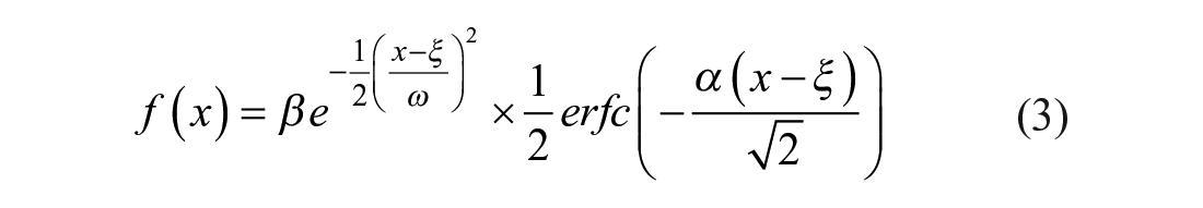
f (x) = β e^{- \frac{1}{2} {(\frac{x - ξ}{ω})}^{2}} \times \frac{1}{2} e r f c (- \frac{α (x - ξ)}{\sqrt{2}})

(3)

where β is the amplitude, ξ is a location parameter, ω is a scale parameter, erfc is the complementary error function, and α is a shape parameter, such that α > 0 produces a right-skewed peak, α < 0 gives a left-skewed peak, and α = 0 returns a nonskewed Gaussian peak. We calculate the AUC by summing between $ξ \pm 2 \frac{ω}{\sqrt{2}} .$ With 400 simulated skewed Gaussian peaks (with hard-coded background and random noise) and user input random variation in peak location and width, we find an average fit R² value of 0.98 ± 0.01 (standard deviation).

To assess user-to-user variation in analysis of the simulated skewed Gaussian image, the four users performed Summit analysis with skewed Gaussian peak fitting ( Fig. 3E ). Here, all lanes of the simulated image pass quality control, so variation between users represents the impact of steps such as ROI generation, peak boundary selection (which aids in parameter estimation for the fits), and how robustly the peak fitting identifies bounds for AUC integration. The CQVs varied by <0.2% and the Kruskal–Wallis p value was 0.98, indicating that skew peak analysis is highly reproducible across users.

Finally, to benchmark Summit’s quantitative accuracy in assessing peak AUC variation, we carried out Summit and CellProfiler analysis on the simulated skewed Gaussian peak image. Among various batch image processing tools, we selected CellProfiler because it includes an example pipeline for skewed electrophoresis peak analysis from Comet assay gels (in which skewed DNA peaks randomly distributed across the gel report the degree of DNA damage from each single cell). Importantly, CellProfiler does not report metrics that readily allow protein sizing (peak locations relative to a common separation axis origin, e.g., microwell), but the image segmentation utilized in CellProfiler does report integrated fluorescence intensities for each background-subtracted peak in the gel. The calculated AUCs from Summit and CellProfiler are not directly comparable because of the 1D averaging of the ROI performed in Summit. Thus, we aimed to assess normalized AUC distributions (AUC for each peak divided by the mean AUC for all 400 simulated peaks) calculated by Summit and CellProfiler ( Fig. 3F ). The normalized AUC distributions are not statistically significantly different (Mann–Whitney p = 0.82). However, CellProfiler reports slightly lower CQVs in the normalized AUC (2.34% vs 3.01%). Thus, Summit quantifies AUC variation from Gaussian fitting of 1D intensity profiles that is in agreement with established batch image processing tools, while Summit is equipped to report separation metrics (e.g., estimated protein molecular mass or separation resolution between two peaks).

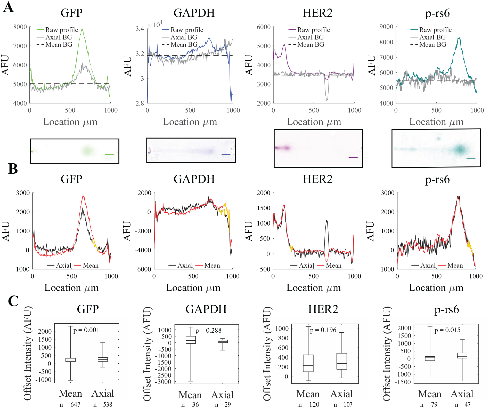
Comparing Efficacy of Mean versus Axial Background Subtraction

We investigated two local approaches for background subtraction for each individual ROI: (1) mean background subtraction (which closely resembles average on-boundary background subtraction in 2D electrophoresis³¹) and (2) axial background subtraction (employed in our previous work²¹). The background subtraction methods are compared with EP cytometry of four example proteins: GFP and GAPDH (from MCF7 breast cancer cell lines) and HER2 and p-rs6 (from patient-derived breast cancer tumor tissue; data made publicly available previously²⁰) in Figure 4 . Once each ROI is segmented, we generate 1D intensity profiles from each 2D EP cytometry image. This is achieved by averaging each pixel along the width of the ROI, which collapses the 2D image to a 1D raw profile ( Fig. 4A ). Both subtraction methods take “gutter” regions directly adjacent to the separation lane as the background region ( Suppl. Fig. S4 ). For mean background subtraction, all pixels within the two gutters are averaged ( Fig. 4A ) and the average value is subtracted from the 1D profile ( Fig. 4B ). Axial background subtraction calculates an average gutter background at every position along the length of the separation lane ( Fig. 4A ). For example, for a typical 5-pixel gutter width, 10 total pixels are averaged and that average value is subtracted from the corresponding intensity value at that location along the separation axis ( Fig. 4B ).

Figure 4.

Comparison of mean and axial background subtraction for Western blot intensity profile background subtraction in Summit. (A) Raw intensity profiles, axial background (BG), and mean BG and false-colored fluorescence micrographs for GFP, GAPDH, HER2, and p-rs6. Scale bar = 100 μm. (B) Intensity profile of the raw profile in A with axial or mean background subtraction. The region of the profile used to calculate the offset intensity is shown in gold. (C) Box plot quantitation of the median of the offset intensity of the intensity profiles with axial or mean background subtraction. Mann–Whitney p values are shown.

In order to assess the efficacy of background subtraction, we introduce a method to quantify how well each method brings the protein peak baseline to zero. We quantified the median of an offset region of the intensity profile outside of the peak area (i.e., 2 to 3 σ from the peak center; outlined in gold in Fig. 4B ). The offset intensity is lower when using mean background subtraction for GFP (median offset, 218 vs 258; Mann–Whitney p = 0.001; Cohen’s d < 0.01) and p-rs6 (median offset, 69 vs 159; Mann–Whitney p = 0.015; Cohen’s d < 0.01, Fig. 4C ). Corroborating this result, the number of peaks that pass quality control is ~11%–50% higher for mean instead of axial subtraction.

Automated Gaussian Curve Fitting for Thousands of Peak Intensity Profiles

In order to improve the quality of the Gaussian fit, the region of the intensity profile to be fit must be selected, and initial guesses for each of the fit parameters must be provided. The manual peak bound selection with an overlaid plot of all electropherograms was previously described for high-throughput microfluidic capillary electrophoresis¹⁷ and is employed here for thousands of separations ( Suppl. Fig. S5 ). The constraints for the parameters are 0 < a < a_max (where a_max is the maximum intensity across all of the intensity profiles), left bound < μ < right bound, and 0 < b < right bound – left bound. MATLAB uses a least-squares curve-fitting algorithm for Gaussian fitting of each curve. If an estimated signal-to-noise (SNR) threshold is provided, only intensity profiles with an estimated SNR ratio >3 are fit to the Gaussian function. Goodness-of-fit metrics such as the R² value and confidence intervals for each fit parameter are stored in the results data structure.

Increasing the goodness of the Gaussian fit improves the measurement of molecular mass and quantity of a detected protein. The R² values of the Gaussian fit were lower with axial subtraction than with mean subtraction, except for the HER2 peaks ( Fig. 5 A, B ). The largest difference in R² values between the two background subtraction methods was with the skewed GAPDH peaks (median R² = 0.71 and 0.81 for axial and mean subtraction, respectively). GAPDH and HER2 had statistically significantly lower R² values than GFP or p-rs6 with mean subtraction (Kruskal–Wallis p < 0.0001; Dunn–Sidak multiple comparison test p < 0.0001 for each pairwise comparison except for GAPDH and HER2, p = 0.14; all sample sizes shown in Fig. 5B ). The median R² values for GAPDH and HER2 were 0.71 and 0.88, respectively. For a more specific assessment of fit performance, we quantified the uncertainty in the fit parameters. We calculated the percent variation between each fit parameter and the lower bound of the parameter’s 95% confidence interval and found that the uncertainty decreases with increasing R² value, as anticipated ( Fig. 5B ). For example, the percent variation in peak width is

% v a r i a t i o n σ = \frac{σ - σ_{c i}}{σ} \times 100

(4)

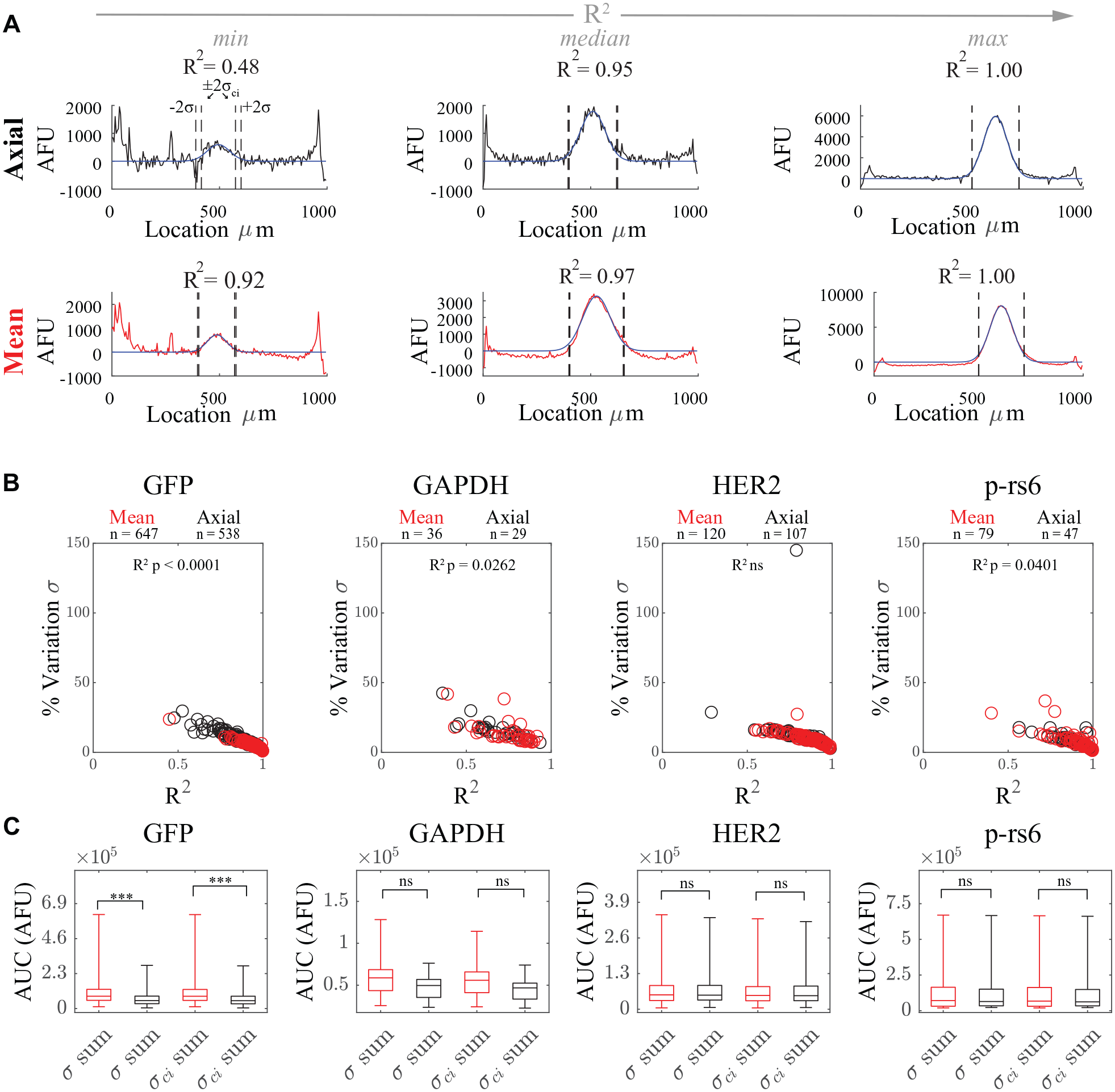
The parameter with the smallest percent variation is the peak center ( Suppl. Fig. S6 ), which largely differed by <5%. In contrast, for the majority of peaks with a fit R² value <0.8, the percent variation in the peak width is >10% ( Fig. 5B ).

Figure 5.

Quantitative assessment of goodness of Gaussian fitting and AUC dependence on mean versus axial background subtraction. (A) Representative intensity profiles (axial subtraction, black trace; mean subtraction, red trace) and Gaussian fit (blue trace) of GFP peaks that passed quality control with the minimum (min), median, or maximum (max) R² value for the axial subtraction set. Black dashed lines indicate the summation bounds for calculating the AUC from the peak width, σ (±2σ or ±2σ_ci, where ci corresponds to the 95% confidence interval for the peak width fit parameter). (B) Percent variation between σ and σ_ci as a function-of-fit R² value for mean (red points) and axial (black points) subtraction for the analysis of EP cytometry images of GFP, GAPDH, HER2, and p-rs6. Number of data points and the Mann–Whitney p value for the R² value are shown. (C) Box plot quantification of the AUC with the indicated summation bounds. Red indicates mean background subtraction and black indicates axial background subtraction. The numbers of lanes that passed quality control with both background subtraction methods are n = 523 (GFP), n = 19 (GAPDH), n = 104 (HER2), and n = 45 (p-rs6). Mann–Whitney p value significance levels: ns = not significant, *** p < 0.0001.

Dependence of AUC on Peak Width Parameter Confidence Interval

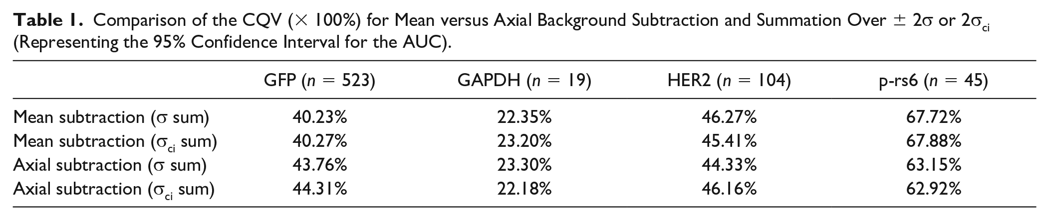
We quantified AUC variation with summation of the background-subtracted intensity profile over μ ± 2σ or μ ± 2σ_ci (which represents a 95% confidence interval for the AUC based on the uncertainty of the peak width fit parameter) as shown in Figure 5A . As shown in Figure 5C and Table 1 , the measured distributions vary minimally based on the background subtraction employed. For all proteins studied here except GFP, we fail to reject the null hypothesis that protein levels measured with mean or axial subtraction are drawn from a single distribution (Mann–Whitney test p > 0.05). The CQV of AUC differed by only a few percent between mean and axial background subtraction for each protein target investigated here. Mean subtraction slightly increases AUC CQV by ~2% and ~4.5%, respectively, for HER2 and p-rs6, while decreasing CQV by ~3.5% and 1% for GFP and GAPDH, respectively. Here, protein variation for GFP, GAPDH, HER2, and p-rs6 is relatively accurately reported when quantified from AUCs with the typical μ ± 2σ summation because CQVs differ by only ~1%–2% when calculated with μ ± 2σ_ci summation bounds instead.

Table 1.

Comparison of the CQV (× 100%) for Mean versus Axial Background Subtraction and Summation Over ± 2σ or 2σ_ci (Representing the 95% Confidence Interval for the AUC).

	GFP (n = 523)	GAPDH (n = 19)	HER2 (n = 104)	p-rs6 (n = 45)
Mean subtraction (σ sum)	40.23%	22.35%	46.27%	67.72%
Mean subtraction (σ_ci sum)	40.27%	23.20%	45.41%	67.88%
Axial subtraction (σ sum)	43.76%	23.30%	44.33%	63.15%
Axial subtraction (σ_ci sum)	44.31%	22.18%	46.16%	62.92%

Discussion

We designed Summit as an automated platform for carrying out analysis of EP cytometry images, storing critical analysis parameters needed for reproducibility and often neglected in Western blot densitometry. Further, we sought to understand how algorithm design decisions, such as a method of background subtraction, affect uncertainty and variation in protein expression. Consequently, we introduce offset intensity as a metric for assessing the efficacy of background subtraction. Additionally, we evaluate the confidence intervals of Gaussian fit parameters and AUCs of protein peaks. While parameters and design choices may need to be tuned for each protein analyzed, we offer guidelines based on increasing the number of quantifiable separations per image and minimizing variation induced by the analysis itself.

User-to-User Variation in Quantitation Is Minimal Owing to Accessibility of Parameters to Reproduce Analysis and Automation

Emerging guidelines for computational research to improve scientific reproducibility³² suggest that individual steps of code that affect the final analysis should be logged.³³ Thus, the choice of how to store output of both the analysis of interest and the variables used to execute the functions is crucial for making a given analysis reproducible.

Even using the same ROIs to segment an EP cytometry image, user-to-user-variation in analysis output can occur owing to manual quality control with optional quantitative thresholds. The optional thresholds include a minimum Gaussian fit R² value (previously recommended at ~0.7) and an SNR ratio estimate >3.²¹ After thresholding, a user may eliminate a given intensity profile for various reasons: (1) punctate fluorescence (e.g., dust or fluorescent antibody aggregates) in the peak region, (2) gel damage in the peak or background region, (3) large fluorescent debris (e.g., fluorescent cell debris) in the peak or background region, (4) unexplained injection dispersion causing peak skew, (5) poor Gaussian fitting resulting in inaccurate peak boundary identification, or (6) peak SNR ratio that is too low. Similar manual inspection and elimination of protein spots for analysis has been applied to regions of reverse-phase protein arrays, prompting concern that user-to-user variation in quality control could yield inconsistent results.³⁴ Here, the slight disparity in CQV (~6.5% for the experimentally collected EP cytometry image) may be attributable to differences in which intensity profiles the users allowed through quality control. When all four users did not agree, the most common feature of the peaks was a lower than average SNR ratio. Inclusion of a more rigorous SNR calculation as part of quality control (which would quantify peak signal as the peak amplitude and noise as the standard deviation of a background region at the edge of the ROI) may reduce user-to-user variation in the assessment of low SNR peaks.

Choice of Background Subtraction Method Impacts Assay Throughput

Background subtraction of protein signal remains a challenge in the quantitative analysis of protein electrophoresis and microarray images.^35,36 The choice of background subtraction method strongly influences the measured quantity of protein¹⁰ and variance. Common background subtraction approaches for electropherograms include rolling ball, baseline, and “on-boundary” (e.g., lowest or average) subtraction.^10,35 The rolling ball method has been shown to yield densitometry protein measurements that are less correlated with a radioimmunoassay than if no background subtraction were performed.¹⁰ Average on-boundary subtraction (the average of a trace just beyond the protein band boundary) in 2D electrophoresis was shown to achieve the lowest overall protein coefficient of variation in acidic 2D electrophoresis. A similar “neighborhood correction” strategy applied to reverse-phase protein microarrays that suffer from nonuniformities across the array also yielded a lower protein spot coefficient of variation.³⁷ Thus, on-boundary or neighborhood-based subtractions are appealing for both electrophoresis and protein arrays.

Similar to protein microarrays, EP cytometry background subtraction must occur for hundreds to thousands of individual regions across the array. Furthermore, nonuniform background, as observed in gradient gel EP cytometry³⁸ and in 2D gel electrophoresis,³⁹ requires a subtraction other than the straightforward and computationally inexpensive baseline subtraction. Thus, we aimed to identify appropriate local background subtraction methods that could address nonuniform background (across the device or within an ROI), maximize the number of quantifiable peaks, and reduce quantification variance.

Quantifying variation in offset intensity, CQV dependence on subtraction method, and summation bounds, and assessing if higher n reveals otherwise unmeasured cell subpopulations, can aid in the choice of background subtraction best suited for a given protein target and research question. When mean subtraction reduces or only slightly increases the CQV relative to axial subtraction, mean subtraction may be the preferred background subtraction method, as it likely increases n.

Maximizing the fraction of analyzed samples that yield useful data (i.e., pass quality control) is critical in single-cell analysis in order to identify rare cell subpopulations. We hypothesize that mean subtraction yields higher n because the effect of any “hot” pixels in the background gutter region is averaged out with mean subtraction. In the case of cells derived from precious patient tumor samples, maximizing assay quality yield is critical to assess biomarker heterogeneity (like the HER2 and p-rs6 analyzed here) that may dictate whether a chemotherapy drug is effective or not.²⁰ Thus, further refining the background subtraction process to maximize n is an important future direction.

As new data types may benefit from alternative background subtraction methods tailored to the features of the background, Summit includes an optional input to the intProf function in which the user may supply their own background subtraction function. Such custom functions will be especially useful for low-abundance proteins, for which low peak SNR ratios may result from averaging to generate the 1D intensity profile. Additionally, low SNR ratio peaks may benefit from denoising algorithms employed in 2D electrophoresis,⁴⁰ such as nonlinear filtering.⁴¹

Narrow Confidence Intervals of Fit Parameters Indicate Analysis Contributes Minimally to Technical Variation of Quantified Peak AUC or Location

While offset intensity is different between mean and axial subtraction, we only expect differences in variation of offset intensity, not magnitude, to result in altered AUC variation. Thus, to truly understand whether either axial or mean background subtraction is associated with higher protein variation, we also directly compared the AUCs with different subtraction methods while evaluating the accuracy of AUC determination. We hypothesize that mean and axial subtraction yield different GFP AUC distributions because of the bleed-through of GFP signal into the background region seen in Figure 4A .

Accurate quantitation of peak width and location parameters is critical for the determination of protein size,⁴² separation performance (e.g., separation resolution), and summation bounds for the AUC. Here, AUC is determined from the background-subtracted intensity profile,⁴³ as AUC quantification directly from the Gaussian fit is preferable for peaks with substantial overlap. We hypothesized that higher uncertainty of the peak width parameter may reduce accuracy of the AUC for lower R² fits. We found that GAPDH and HER2 had the lowest median R² values, which results from the lower SNR ratio of the GAPDH peaks and notable injection dispersion for HER2 shown in Figure 4A . However, the uncertainty of the peak width parameter for these lower R² peaks did not lead to statistically significant differences in the AUCs when summing over μ ± 2σ versus μ ± 2σ_ci (Mann–Whitney p > 0.05). Thus, Summit quantifies these examples of peaks with lower SNR ratio or dispersion without higher uncertainty in the AUC.

Quantitative analysis of EP separation data can reveal the presence and abundance of proteoforms responsible for biological processes such as cancer progression.^44–47 Summit provides reproducible quantitation by storing all critical parameters and output variables in the results data structure. Further, automating most aspects of the analysis and quality control reduces user-to-user variation in the analysis results. We found that the differences between quantified protein peak AUC are not statistically significant between Summit users. Minimization of assay technical variation introduced by the algorithm may be achieved by examining variation in background subtraction offset, and CQV variation within the 95% confidence interval of peak bounds. In some instances, there may be a trade-off between the number of analyzed peaks and variation, depending on the background subtraction employed.

For both background subtraction methods explored here, punctate noise in the vicinity of the peak or background “gutter region” is a common feature that prevents certain peaks from passing quality control. We are investigating 2D segmentation methods that may improve yield by isolating the antibody signal from the punctate nonspecific signals on the periphery of the separation lane. Improving assay quality yield would enhance the ability of EP separation methods to detect rare cell populations.

Owing to the modular design of Summit, we anticipate components such as the ROI generation and intensity profile background subtraction could be applied to other arrayed separations and detection of different biomolecules. To date, the algorithm has been applied to both size-based separations in custom lab-on-a-disk devices⁴⁸ and single-cell isoelectric focusing assays.¹⁶ For the latter, geometric differences between the 1-mm-long EP cytometry separation lanes and 9-mm-long focusing zones were readily modified, as the parameters defining the geometry of the separation array are Summit input variables. Given the ease of adapting the analysis to other geometries, Summit could likely also be used for standard Western blotting densitometry. We anticipate that the skewed Gaussian function included in Summit could be applied to commonly skewed data types such as the arrayed comet assay for DNA damage.¹⁵ Further, addition of an alternate skewed fit function, such as the Lorentzian-modified Gaussian,^49,50 could allow application of Summit to chromatography data.

In the future, Summit-extracted peak shape parameters may shed insight on proteins that are poorly solubilized in EP cytometry (e.g., proteins originating from circulating tumor cells⁵¹). Metrics of EP injection dispersion may guide optimization of sample preparation. For example, we envision identifying effective denaturation conditions for EP cytometry tuned to different classes of protein domain structures⁵² based on peak skew, variance, and quantity of signal entrapped at the microwell interface. Such quantitative analysis will broaden the applicability of EP cytometry to new sample types and protein targets.

Supplemental Material

sj-pdf-1-jla-10.1177_24726303211036869 – Supplemental material for Summit: Automated Analysis of Arrayed Single-Cell Gel Electrophoresis

Supplemental material, sj-pdf-1-jla-10.1177_24726303211036869 for Summit: Automated Analysis of Arrayed Single-Cell Gel Electrophoresis by Julea Vlassakis, Kevin A. Yamauchi and Amy E. Herr in SLAS Technology

Footnotes

Acknowledgements

We are grateful to current and former Herr lab members, and students from the Cold Spring Harbor Labs Single-Cell Analysis Course for user feedback on Summit. We acknowledge Ms. Anjali Gopal and Mr. Andoni Mourdoukoutas for their contributions to reproducibility analyses.

Supplemental material is available online with this article.

Declaration of Conflicting Interests

The authors declared the following potential conflicts of interest with respect to the research, authorship, and/or publication of this article: The authors acknowledge competing financial interest(s) as follows: J.V., K.A.Y., and A.E.H. are inventors of EP cytometry intellectual property and may benefit from licensing royalties.

Funding

The authors disclosed receipt of the following financial support for the research, authorship, and/or publication of this article: This work was partially supported by the Society of Lab Automation and Screening Graduate Education Fellowship (J.V.), NSF Graduate Fellowship DGE1106400 (J.V., K.A.Y.), NSF CAREER CBET1056035 (A.E.H.), and NIH R01CA203018 (A.E.H.).

ORCID iDs

Julea Vlassakis

Amy E. Herr

References

Toby

T. K.

Fornelli

Kelleher

N. L.

Progress in Top-Down Proteomics and the Analysis of Proteoforms. Annu. Rev. Anal. Chem. 2016, 9, 499–519.

Burnette

W. N.

“Western Blotting”: Electrophoretic Transfer of Proteins from Sodium Dodecyl Sulfate-Polyacrylamide Gels to Unmodified Nitrocellulose and Radiographic Detection with Antibody and Radioiodinated Protein A. Anal. Biochem. 1981, 112, 195–203.

Wenisch

de Besi

Righetti

P. G.

Conventional Isoelectric Focusing and Immobilized PH Gradients in ‘Macroporous’ Polyacrylamide Gels. Electrophoresis 1993, 14, 583–590.

Righetti

P. G.

Caravaggio

Isoelectric Points and Molecular Weights of Proteins. J. Chromatogr. A 1976, 127, 1–28.

Herr

A. E.

Singh

A. K.

Photopolymerized Cross-Linked Polycrylamide Gels for On-Chip Protein Sizing. Anal. Chem. 2004, 76, 4727–4733.

Jin

Furtaw

M. D.

Chen

, et al. Multiplexed Western Blotting Using Microchip Electrophoresis. Anal. Chem. 2016, 88, 6703–6710.

Anderson

G. J.

M Cipolla

Kennedy

R. T.

Western Blotting Using Capillary Electrophoresis. Anal. Chem. 2011, 83, 1350–1355.

Bharadwaj

Santiago

J. G.

Mohammadi

Design and Optimization of On-Chip Capillary Electrophoresis. Electrophoresis 2002, 23, 2729–2744.

Mellors

J. S.

Jorabchi

Smith

L. M.

, et al. Integrated Microfluidic Device for Automated Single Cell Analysis Using Electrophoretic Separation and Electrospray Ionization Mass Spectrometry. Anal. Chem. 2010, 82, 967–973.

10.

Gassmann

Grenacher

Rohde

, et al. Quantifying Western Blots: Pitfalls of Densitometry. Electrophoresis 2009, 30, 1845–1855.

11.

Duncombe

T. A.

Herr

A. E.

Photopatterned Free-Standing Polyacrylamide Gels for Microfluidic Protein Electrophoresis. Lab Chip 2013, 13, 2115–2123.

12.

Pan

Sackmann

E. K.

Wypisniak

, et al. Determination of Equilibrium Dissociation Constants for Recombinant Antibodies by High-Throughput Affinity Electrophoresis. Sci. Rep. 2016, 6, 39774.

13.

Hughes

A. J.

Spelke

D. P.

, et al. Single-Cell Western Blotting. Nat. Methods 2014, 11, 749–755.

14.

Gutzweiler

Gleichmann

Tanguy

, et al. Open Microfluidic Gel Electrophoresis: Rapid and Low Cost Separation and Analysis of DNA at the Nanoliter Scale. Electrophoresis 2017, 38, 1764–1770.

15.

Wood

D. K.

Weingeist

D. M.

Bhatia

S. N.

, et al. Single Cell Trapping and DNA Damage Analysis Using Microwell Arrays. Proc. Natl. Acad. Sci. U.S.A. 2010, 107, 10008–10013.

16.

Tentori

A. M.

Yamauchi

K. A.

Herr

A. E.

Detection of Isoforms Differing by a Single Charge Unit in Individual Cells. Angew. Chem. Int. Ed. 2016, 55, 12431–12435.

17.

Shackman

J. G.

Watson

C. J.

Kennedy

R. T.

High-Throughput Automated Post-Processing of Separation Data. J. Chromatogr. A 2004, 1040, 273–282.

18.

Weingeist

D. M.

Wood

D. K.

, et al. Single-Cell Microarray Enables High-Throughput Evaluation of DNA Double-Strand Breaks and DNA Repair Inhibitors. Cell Cycle 2013, 12, 907–915.

19.

Ngo

L. P.

Owiti

N. A.

Swartz

, et al. Sensitive CometChip Assay for Screening Potentially Carcinogenic DNA Adducts by Trapping DNA Repair Intermediates. Nucleic Acids Res. 2020, 48, e13.

20.

Kang

C.-C.

Ward

T. M.

Bockhorn

, et al. Electrophoretic Cytopathology Resolves ERBB2 Forms with Single-Cell Resolution. NPJ Precis. Oncol. 2018, 2, 10.

21.

Kang

C.-C.

Yamauchi

K. A.

Vlassakis

, et al. Single Cell-Resolution Western Blotting. Nat. Protoc. 2016, 11, 1508–1530.

22.

Mcquin

Goodman

Chernyshev

, et al. CellProfiler 3.0: Next-Generation Image Processing for Biology. PLoS Biol. 2018, 16, e2005970.

23.

Berg

Kutra

Kroeger

, et al. Ilastik: Interactive Machine Learning for (Bio)Image Analysis. Nat. Methods 2019, 16, 1226–1232.

24.

Perkel

Starfish Enterprise: RNA Goes Spatial. Nature 2019, 572, 549–551.

25.

Yamauchi

Herr

Sub-Cellular Western Blotting of Single Cells. Microsyst. Nanoeng. 2017, 3, 16079.

26.

Jackson

Browell

Gautrey

, et al. Clinical Significance of HER-2 Splice Variants in Breast Cancer Progression and Drug Resistance. Int. J. Cell Biol. 2013, 2013, 1–8.

27.

Giddings

J. C.

Unified Separation Science. John Wiley & Sons: New York, 1991; pp 97–101.

28.

Glantz

Primer of Biostatistics, 6th Ed. McGraw Hill Professional: New York, 2005.

29.

Cai

Friedman

Xie

X. S.

Stochastic Protein Expression in Individual Cells at the Single Molecule Level. Nature 2006, 440, 358–362.

30.

Bonett

D. G.

Confidence Interval for a Coefficient of Quartile Variation. Comput. Stat. Data Anal. 2006, 50, 2953–2957.

31.

Wheelock

Å. M.

Goto

. Effects of Post-Electrophoretic Analysis on Variance in Gel-Based Proteomics. Expert Rev. Proteomics 2006, 3, 129–142.

32.

Begley

C. G.

Ellis

L. M.

Drug Development: Raise Standards for Preclinical Cancer Research. Nature 2012, 483, 531–533.

33.

Peng

R. D.

Reproducible Research in Computational Science. Science (80-). 2011, 334, 1226–1227.

34.

Liu

Roebuck

P. L.

, et al. Development of a Robust Classifier for Quality Control of Reverse-Phase Protein Arrays. Bioinformatics 2015, 31, 912–918.

35.

Wheelock

Å. M.

Buckpitt

A. R

. Software-Induced Variance in Two-Dimensional Gel Electrophoresis Image Analysis. Electrophoresis 2005, 26, 4508–4520.

36.

Shannon Neeley

Baggerly

K. A.

Kornblau

S. M

. Surface Adjustment of Reverse Phase Protein Arrays Using Positive Control Spots. Cancer Inform. 2012, 11, 77–86.

37.

Zhu

Gerstein

Snyder

ProCAT: A Data Analysis Approach for Protein Microarrays. Genome Biol. 2006, 7, R110.

38.

Duncombe

T. A.

Kang

C.-C.

Maity

, et al. Hydrogel Pore-Size Modulation for Enhanced Single-Cell Western Blotting. Adv. Mater. 2015, 28, 327–334.

39.

Berth

Moser

F. M.

Kolbe

, et al. The State of the Art in the Analysis of Two-Dimensional Gel Electrophoresis Images. Appl. Microbiol. Biotechnol. 2008, 79, 329.

40.

Goez

M. M.

Torres-Madroñero

M. C.

Röthlisberger

, et al. Preprocessing of 2-Dimensional Gel Electrophoresis Images Applied to Proteomic Analysis: A Review. Genom. Proteom. Bioinforma 2018, 16, 63–72.

41.

Tsakanikas

Manolakos

Effective Denoising of 2D Gel Proteomics Images Using Contourlets. In 2007 IEEE International Conference on Image Processing, San Antonio, TX, Sept 16–19, 2007; IEEE: Piscataway, NJ, 2007; pp 269–272.

42.

Kim

J. J.

Chan

P. P. Y.

Vlassakis

, et al. Microparticle Delivery of Protein Markers for Single-Cell Western Blotting from Microwells. Small 2018, 14, e1802865.

43.

Vohradský

Pánek

Quantitative Analysis of Gel Electrophoretograms by Image Analysis and Least Squares Modeling. Electrophoresis 1993, 14, 601–612.

44.

Mitra

Brumlik

M. J.

Okamgba

S. U.

, et al. An Oncogenic Isoform of HER2 Associated with Locally Disseminated Breast Cancer and Trastuzumab Resistance. Mol. Cancer Ther. 2009, 8, 2152–2162.

45.

Solakidi

Psarra

A.-M. G.

Nikolaropoulos

, et al. Estrogen Receptors Alpha and Beta (ERalpha and ERbeta) and Androgen Receptor (AR) in Human Sperm: Localization of ERbeta and AR in Mitochondria of the Midpiece. Hum. Reprod. 2005, 20, 3481–3487.

46.

Okoro

D. R.

Rosso

Bargonetti

Splicing up Mdm2 for Cancer Proteome Diversity. Genes Cancer 2012, 3, 311–319.

47.

Rajan

Elliott

D. J.

Robson

C. N.

, et al. Alternative Splicing and Biological Heterogeneity in Prostate Cancer. Nat. Rev. Urol. 2009, 6, 454–460.

48.

Kim

J. J.

Sinkala

Herr

A. E.

High-Selectivity Cytology via Lab-on-a-Disc Western Blotting of Individual Cells. Lab Chip 2017, 17, 855–863.

49.

Caballero

R. D.

Garcıa-Alvarez-Coque

M. C.

Baeza-Baeza

J. J.

Parabolic-Lorentzian Modified Gaussian Model for Describing and Deconvolving Chromatographic Peaks. J. Chromatogr. A 2002, 954, 59–76.

50.

Shadle

S. E.

Allen

D. F.

Guo

, et al. Quantitative Analysis of Electrophoresis Data: Novel Curve Fitting Methodology and Its Application to the Determination of a Protein-DNA Binding Constant. Nucleic Acids Res. 1997, 25, 850–860.

51.

Sinkala

Sollier-Christen

Renier

, et al. Profiling Protein Expression in Circulating Tumour Cells Using Microfluidic Western Blotting. Nat. Commun. 2017, 8, 14622.

52.

Orengo

Michie

Jones

, et al. CATH—A Hierarchic Classification of Protein Domain Structures. Structure 1997, 5, 1093–1108.

Supplementary Material

Please find the following supplemental material available below.

For Open Access articles published under a Creative Commons License, all supplemental material carries the same license as the article it is associated with.

For non-Open Access articles published, all supplemental material carries a non-exclusive license, and permission requests for re-use of supplemental material or any part of supplemental material shall be sent directly to the copyright owner as specified in the copyright notice associated with the article.

0.00 MB

1.64 MB