
Abstract
A digital assay is one in which the sample is partitioned into many small containers such that each partition contains a discrete number of biological entities (0, 1, 2, 3, …). A powerful technique in the biologist’s toolkit, digital assays bring a new level of precision in quantifying nucleic acids, measuring proteins and their enzymatic activity, and probing single-cell genotypes and phenotypes. Part I of this review begins with the benefits and Poisson statistics of partitioning, including sources of error. The remainder focuses on digital PCR (dPCR) for quantification of nucleic acids. We discuss five commercial instruments that partition samples into physically isolated chambers (cdPCR) or droplet emulsions (ddPCR). We compare the strengths of dPCR (absolute quantitation, precision, and ability to detect rare or mutant targets) with those of its predecessor, quantitative real-time PCR (dynamic range, larger sample volumes, and throughput). Lastly, we describe several promising applications of dPCR, including copy number variation, quantitation of circulating tumor DNA and viral load, RNA/miRNA quantitation with reverse transcription dPCR, and library preparation for next-generation sequencing. This review is intended to give a broad perspective to scientists interested in adopting digital assays into their workflows. Part II focuses on digital protein and cell assays.
Introduction
For the purposes of this article, we define a biological assay as the quantification of the concentration or activity of a biological entity in a sample container. A digital assay is one in which the sample is first partitioned into many small containers such that each partition contains a discrete number of biological entities (0, 1, 2, 3, …). The term digital assay should not be confused with digital microfluidics 1 or single-molecule imaging techniques,2–4 which are reviewed elsewhere.
Digital versus Analog Assays
Figure 1 compares a conventional analog assay with a digital assay. Analog assays, typically performed in a vial or a microplate, provide a readout signal A proportional to the bulk sample concentration C. Readout is commonly performed using spectrophotometry, fluorimetry, or nonoptical methods. For example, fluorescence intensity emitted from a probe may be used to quantify the concentration of DNA, or the enzymatic activity of a protein kinase. By contrast, in a digital assay, the sample is first diluted and partitioned into small containers such that each partition contains a discrete number of biological entities. Each partition is individually assayed, giving a 0 or 1 result if any molecules are present. One common misconception is that digital assays require a limiting dilution where each container has either zero or one molecules. 5 While this can be done, it is generally more efficient to have higher loading factors. Exploiting Poisson statistics, digital assays can perform precise counting with as many as six entities per partition, although the noise increases at high loading factors. The sample concentration can be estimated by counting the fraction of empty partitions E (see below).
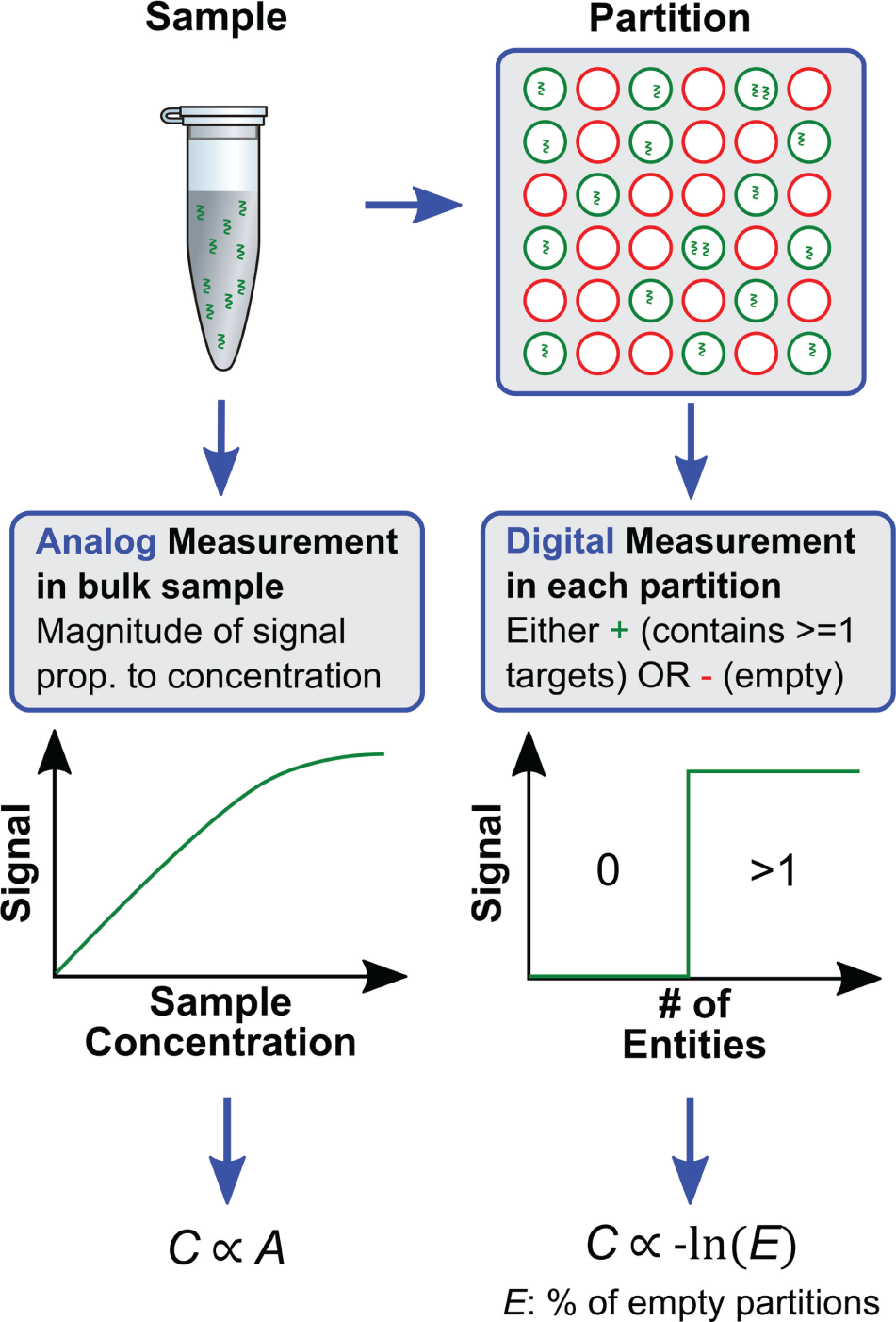
Comparison of digital assays vs. conventional analog biological assays.
The term digital assay originates from the field of digital computers, where computations performed in logic circuits give one of two possible binary outputs. Digital signals are used extensively throughout engineering, particularly in computation and wireless communications. In each case, the information is encoded in a series of ones and zeros. The advantage of digital signals is the reduced burden on detection elements; each needs only to distinguish between two signals: high and low. When this concept is carried over into biological sensors, it simplifies instrumentation—the sensor needs only to tell the difference between a positive and negative partition. The ratio of positive to negative partitions can then be related to the number of molecules in the sample, using Poisson statistics.
Benefits of Partitioning
Partitioning provides several benefits to digital assays over their conventional counterparts, particularly as the number of partitions increases and the partition volumes become small. Two notable effects of partitioning are illustrated in Figure 2 . The first of these is the concentration effect: the limit of detection (LOD) is improved because a small reaction volume increases the effective concentration of the target molecule. 5 This makes it possible, for example, to amplify and detect single molecules of DNA6–8 and single-cell secretions to the extracellular environment.9–11 The second of these, the enrichment effect, improves the analysis of complex mixtures by purifying the target of interest from interfering compounds. More specifically, it increases the ratio of the target of interest versus the background. In an illustrative example ( Fig. 2B ), partitioning results in 8× purification in one replicate, and complete purification in another replicate. In digital PCR (dPCR), the enrichment effect improves amplification efficiency of low-abundance mutant nucleotides against a wild-type background, which is useful for applications like cancer diagnostics. 12 The concentration effect scales inversely with sample volume, while the enrichment effect scales with the number of partitions. A third benefit of partitioning is that a digital assay provides superior precision and linearity when counting copies of targets, simply because it measures individual molecules rather than an ensemble concentration. Precision improves with the number of partitions, since more single entities can be resolved within a large population. Finally, increasing the number of partitions extends the dynamic range, that is, the range of sample concentration that can be measured.
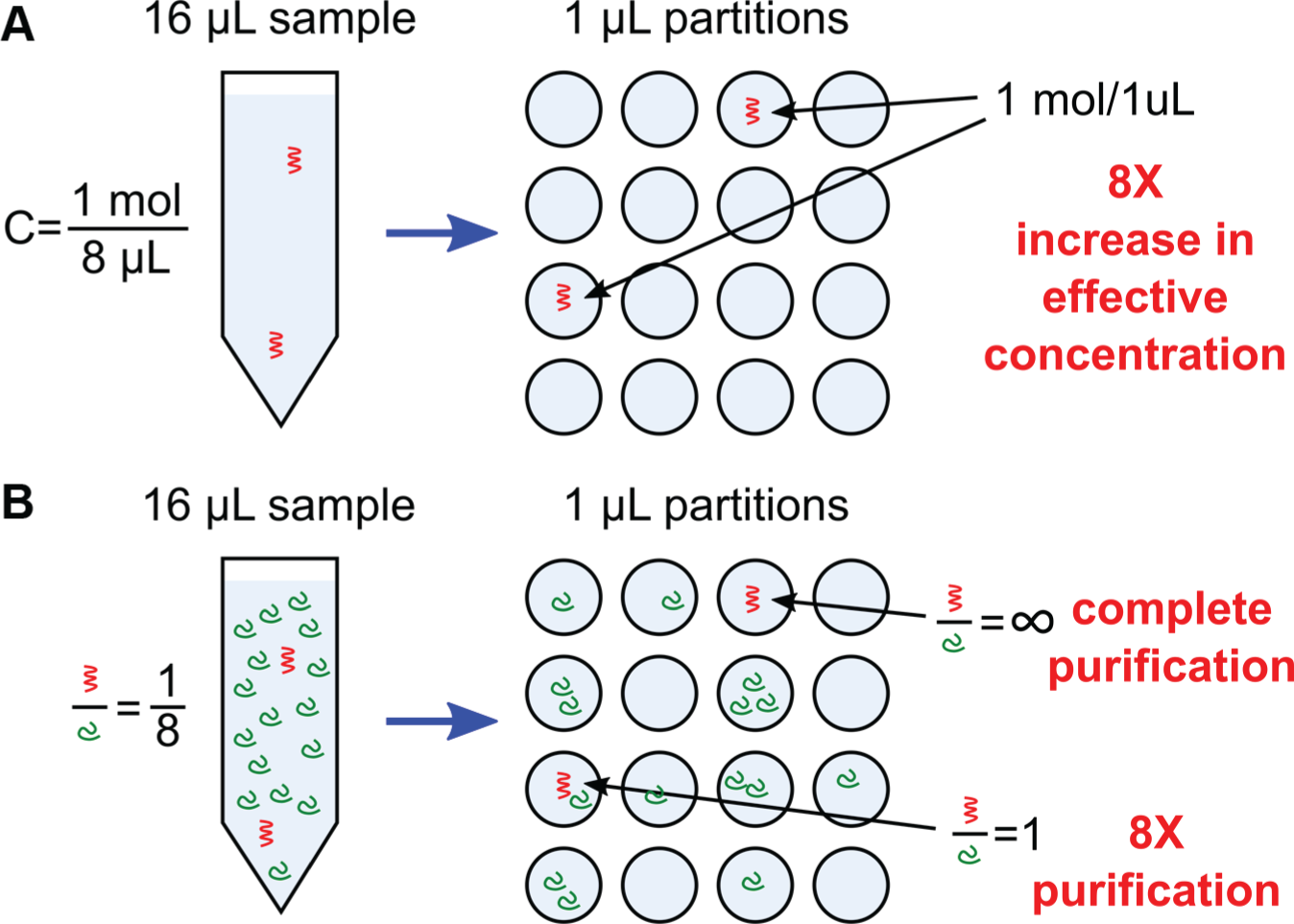
Benefits of partitioning in digital assays. Shown are two illustrative examples: (
Partitioning Methods: Chambers and Droplets
Partitioning is accomplished using two general approaches: (1) arrays of physically isolated chambers or wells or (2) droplet emulsions where the reaction is conducted in water droplets separated by a continuous oil phase. Either approach can provide partition volumes ranging from femtoliters to almost microliter volumes.
In the case of chamber arrays, digital assays have been conducted in commercially available 96-, 384-, or 1536-well plates. However, as described above, scaling to more wells improves the dynamic range and the ability to enrich mutant samples. Scaling can be achieved by miniaturizing the wells using photolithographic and microfabrication processes. For example, photolithography and silicon etching have been used to fabricate 50,000 wells for digital enzyme-linked immunosorbent assay (ELISA), each with a 50 fL volume. 13 Similar platforms for performing digital enzyme assays, with wells designed to accommodate 1.4 fL volumes, have also been fabricated by micromolding a flexible elastomer (PDMS) against a 1 µm silicon structure. 14 Chamber arrays can also be made in plastics using micromolding 15 or imprint lithography,16,17 and in other materials using variants of soft lithography. 18 The resolution of the manufacturing process determines volume variability. Using photolithography, tolerances can be as small as hundreds of nanometers, and with nanoscale imprint lithography, they can be <25 nm. Volume variability contributes to uncertainty in digital counting assays, as described in the next section.
The second approach for partitioning utilizes droplet emulsions in oil. Monodisperse droplets can be made using microfluidic t-junctions where an aqueous stream is combined with a stream of oil, 19 or by flow-focusing cross-geometries where the aqueous stream is combined with two orthogonal streams of oil. 20 The oil should be nonreactive and have low solubility to prevent the diffusion of reactants between reactors; often, fluorocarbon oils are chosen for this purpose. Stable droplet generation requires the addition of surfactants to stabilize the water oil interface and prevent droplet coalescence.21–24 The surfactant must be optimized so that it does not interfere with the assay, and keeps small biomolecules from diffusing into the oil. For more details on droplet microfluidics, the reader is referred to several excellent reviews on the subject, including a comprehensive 2012 review by Guo et al. 25 and a 2010 review by Theberge et al. 26 Tran et al.’s 2013 27 and Teh et al.’s 2008 28 reviews cover technical developments in droplet microfluidics technology, including droplet processing components and their integration in laboratory workflows. Lagu et al.’s 2013 29 and Zagnoni and Cooper’s 2011 30 reviews focus on the application of droplet microfluidics for single-cell biology, highlighting the physics of droplet formation and manipulation, cell encapsulation methods, a variety of sensing and sorting methods, and the use of confinement in single-cell analysis.
Each of the two approaches (chambers or droplets) has its respective benefits. In general, the advantage of droplet systems is that they can generate as many partitions as needed. Droplet dPCR (ddPCR) systems, for example, can provide as many as 10 million partitions. However, droplets are generated serially, which requires minutes to hours to generate sufficient partitions. Step emulsification systems address this issue by massive parallelization, allowing them to generate tens of thousands of droplets in minutes while maintaining relatively uniform droplet size.31,32 The volume uncertainty in droplet systems is due to the polydispersity of droplet generators, usually <5%, while volume uncertainty for lithographically defined chambers is determined by the manufacturing tolerances, as described above. For example, commercial dPCR systems using chamber and droplet implementations typically have <3% uncertainty. 33 In either implementation, care must be taken to avoid adsorption of biomolecules to the interfaces, which can lead to sample loss or enzyme deactivation. Physical chambers can be coated with blocking agents (e.g., bovine serum albumin) to prevent the adsorption and deactivation of biomolecules. 14 Similarly, droplet systems can utilize amphiphilic surfactants, which present a blocking group such as polyethylene glycol (PEG) facing the aqueous side, and a hydrophobic tail facing the oil side.22,24,34
Organization and Scope of This Review
This two-part review article will cover the most popular types of digital assays, including nucleic acids (dPCR), proteins (digital ELISA and enzymatic activity), and cells (single-cell gene expression, proteomics, and transcriptomics). The large variety of assays is accompanied by an equally wide range of applications, each of which will be covered in the respective sections. Part I covers partitioning statistics, and then moves on to dPCR concepts, systems, and applications. Part II 35 discusses digital protein assays, digital cell assays, and their respective applications. Given the readership of SLAS journals, the intended audience is the scientific community using and developing laboratory automation. Accordingly, the article covers fundamental concepts, the methods and types of digital assays reported in the literature, commercial products, and future trends.
Partitioning Statistics
In digital assays, partitioning statistics are used to determine sample concentrations and confidence intervals. Partitioning the sample into small containers results in a statistical distribution of targets (DNA molecules, proteins, or cells) among the partitions ( Fig. 1 ). Partitioning is similar to aliquotting, a common step in a laboratory workflow; however, the latter typically involves such a large number of targets per aliquot that the statistical variation between samples is ignored. By contrast, in digital assays, the number of targets in the sample (m) is typically less than or on the order of the number of partitions (n). As a result, there is significant statistical variation in the number of molecules per partition. The average number of targets per partition (λ) depends on the sample concentration (C) and the number of partitions (n).
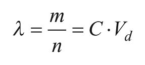
Here, m is the number of targets in the sample and Vd is the partition volume.
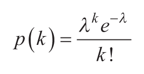
The probability that a partition will contain k copies of the target is governed by the binomial and Poisson distributions. 36 It is worthwhile to understand the intuition behind these distributions, as they are central to digital assays. The binomial distribution is a discrete probability distribution that gives the likelihood of k successes in m trials, each with a probability p. 37 For example, when rolling a die, the binomial distribution gives the probability of rolling a 4 in exactly 7 out of 10 trials. In the case of digital assays, throwing the die is analogous to “throwing” one target entity randomly into an array of partitions, and a success is when a target falls in the selected partition. If there are n partitions, and the partitioning process is perfectly random, the probability that the target appears in the selected partition is 1/n. This trial is repeated m times, once for each molecule in the sample. The binomial distribution, shown below, gives the probability of k successes, that is, the probability that the selected partition contains exactly k molecules.
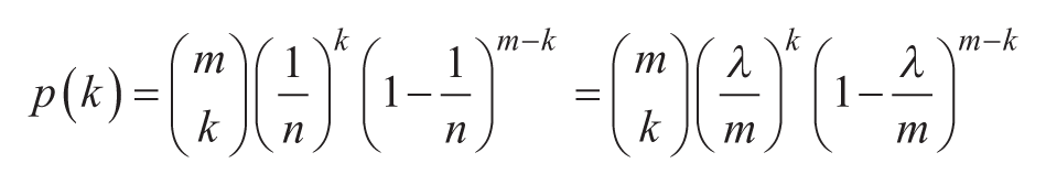
Digital assays typically employ a large number of partitions. When n is large, and the probability of a successful trial (1 / n) is small, the binomial distribution can be approximated by the Poisson distribution.
The mean and variance of the Poisson distribution are both equal to
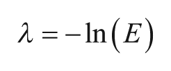
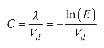
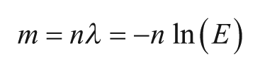
Figure 3 shows calculated Poisson distributions for various values of sample concentration l. As l increases, the proportion of empty partitions falls to zero, making quantitation impossible. To statistically have at least one empty partition (nE > 1), the number of targets must be less than n In (n). 5 This is the ideal limit on the upper dynamic range. In practice, both the upper and lower end of the dynamic range are limited by sources of error.
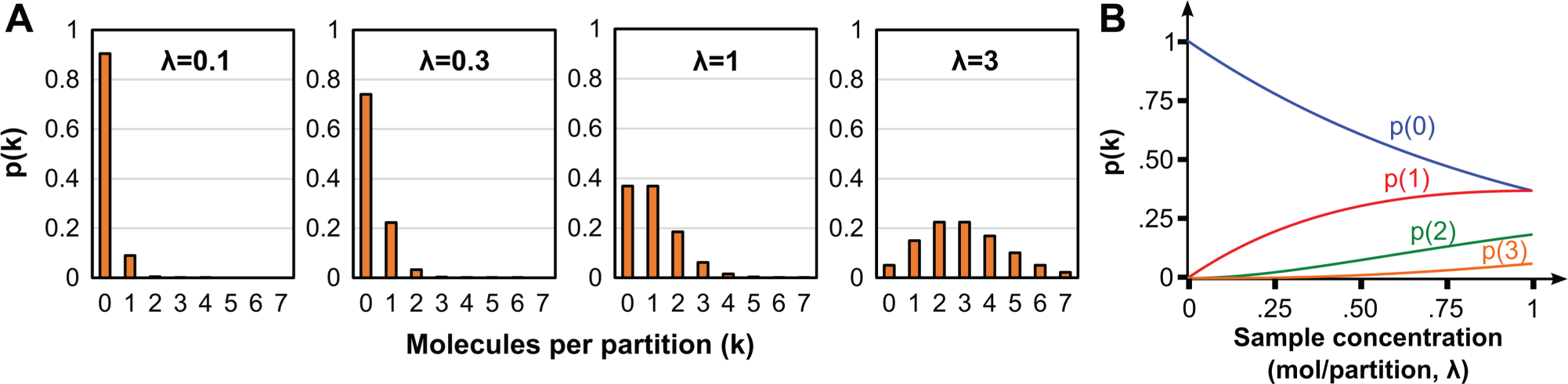
Poisson encapsulation statistics. (
Sources of Error
In conventional analog assays, measurement uncertainty is typically limited by the resolution of the detection instrument ( Fig. 1 ), for example, the ability of a fluorimeter to resolve small differences in emitted fluorescence. In digital assays like dPCR, the detection instrument needs only to identify whether a partition has 0 or >1 targets, which makes data analysis less dependent on the properties of the detector or assay chemistry. Digital assays have two sources of error: subsampling error and partitioning error. 5 Subsampling error sets the lower detection limit at low concentrations and is independent of the instrument, while partitioning error dominates at high concentrations and may depend on the sampling and partitioning instrument.
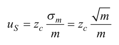
Subsampling errors arise in any biological assay (digital or analog), which does not analyze the full volume of the sample, but rather a subsample of it, resulting in statistical variation between replicate tests. For example, a diagnostic sample like blood serum could be several milliliters, while a typical dPCR system can handle only 20 µL samples. The subsampling process introduces an unavoidable source of error, particularly when there are few targets within the original sample to detect. When subsampling a fraction of a larger sample, the standard deviation of the targets per subsample is
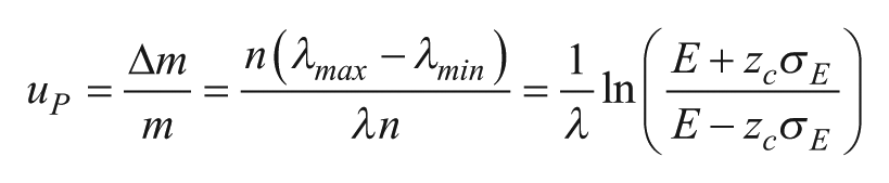
Partitioning errors, which are specific to digital assays, occur because the distribution of targets among partitions may differ from one experiment to the next. In a set of replicate experiments, there is a variance in the number of empty partitions E that propagates to a corresponding variance in the calculated concentration l.
5
An estimate of partitioning error can be found based on the analysis of Dube et al.,
39
which models the partitioning as a binomial process. The standard deviation in the proportion of negative partitions E is
This variation becomes significant at high concentrations (large l), when very few partitions are empty (
Figure 4 compares the relative contributions of subsampling and partitioning errors versus sample concentrations at 20,000 and 1 million partitions. At large l, partitioning error limits the maximum concentration that can be measured, while both errors increase at l < 1. In practice, the sample concentration is chosen to minimize error. For example, in dPCR, the sample concentration is typically adjusted such that l ranges from 0.001 to 65,38 (and in some cases, up to 8 40 ). At n = 1,000,000, the partitioning error drops significantly to <3%, illustrating the benefits of more partitions.
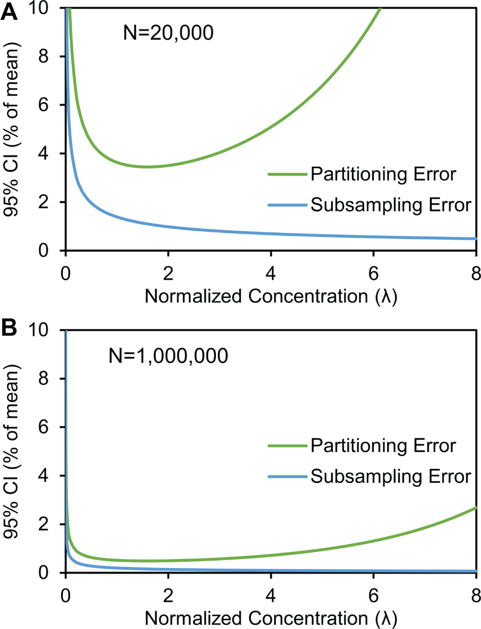
Subsampling errors and partitioning errors in digital assays assuming (
The Poisson model does not take into account variation in partition volume, which can skew the distribution of targets, particularly at high concentrations.12,41 As described by Pinheiro et al.,
42
the volume uncertainty uVd
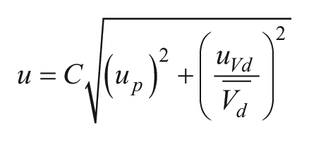
Here,
Digital PCR
The most mature digital assay, digital PCR (dPCR) is a method for absolute quantification of a nucleotide sequence. 5 Although the first paper dates back to 1999, 43 dPCR did not gain widespread use until the first commercial instruments became available in 2007. 44 dPCR is based on the same biochemical principles as quantitative real-time (qPCR), but differs in how quantitation is performed. In qPCR, a sample containing target DNA, PCR reagents, and fluorescent probes is thermally cycled, while monitoring fluorescence at each cycle. During each replication cycle, hydrolysis probes (e.g., Taqman) or intercalating DNA binding dyes (Evagreen or SYBRgreen) exponentially increase fluorescence emission at each cycle, with a rate dependent on amplification efficiency ( Fig. 5 ). Hydrolysis probes release fluorescence when cleaved during each replication cycle, while DNA intercalating dyes increase fluorescence emission when bound to double-stranded DNA. Hydrolysis probes typically offer higher specificity, sensitivity, and quantitation. In all cases, the number of cycles required to achieve a detectable fluorescence, Ct, is related to the number of targets in the original sample.
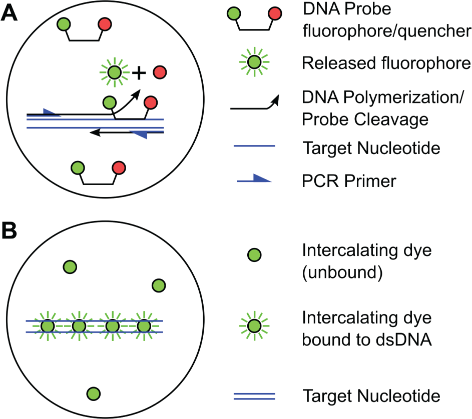
Amplification and detection chemistry in dPCR (same for qPCR). (
In dPCR, the detection chemistry is essentially identical; however, the sample, reagents, and probes are first partitioned into many replicate reactions ( Fig. 1 ), with commercial systems generating between 1000 and 10 million partitions. 43 The partitions are then subjected to excess rounds of thermal cycling (>30), so that any partition that contains one or more DNA targets becomes fluorescent, regardless of amplification efficiency. Then, the proportion of nonfluorescent partitions, through Poisson statistics described above, is used to calculate the target concentration within a well-defined confidence interval.5,39,45 To have a sufficient number of empty partitions, high-concentration samples must first be diluted so that λ is within a range suitable for Poisson quantitation (0.001–6) with tight confidence intervals.5,38
Digital PCR Systems
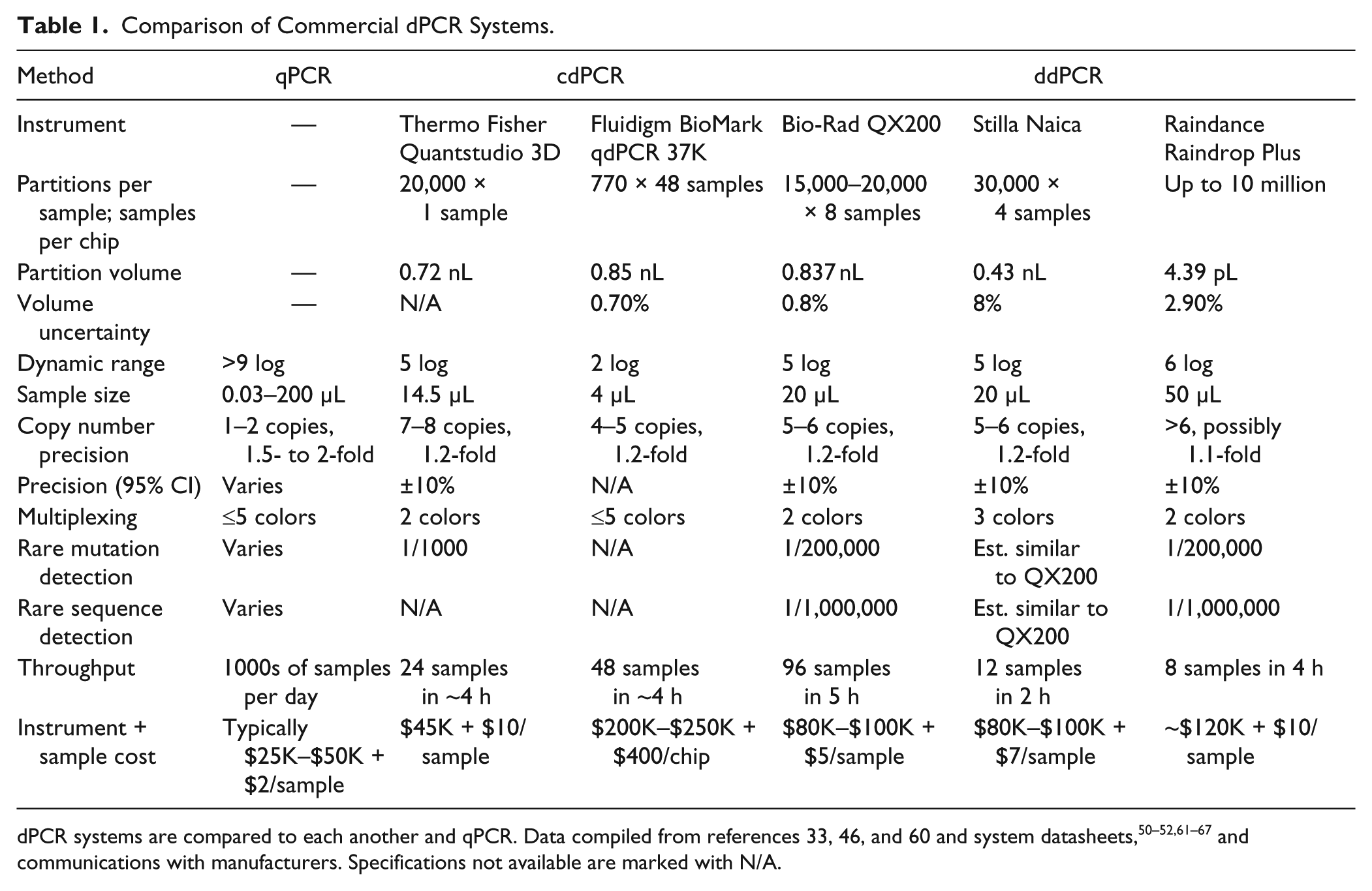
Figure 6 and Table 1 compare five commercially available dPCR systems, which fall into two categories, depending on the way they partition and detect samples. 46 The first category, chamber-based digital PCR (cdPCR) systems, utilize physical structures as partitions. Vogelstein, who coined the term digital PCR in 1999, performed sample partitioning by manually pipetting samples and a PCR mix into a commercial 96-well plate. 43 However, he recognized the benefit of increasing the number of partitions, noting that in 1536-well plates, the theoretical sensitivity in mutation detection would be ~0.1%, and that very high partition systems could be limited only by polymerase errors. True to this assertion, modern cdPCR systems have scaled to more partitions with smaller volumes. For example, Thermo Fisher’s Quantstudio 3D ( Fig. 6B ) is an “open-array plate” that consists of 20,000 thru-holes, each with a diameter of 60 µm, etched through a microscope slide. The inner surfaces are coated with a hydrophilic surface, enabling samples to be loaded via capillary action to form 0.72 nL partitions. The plate is then immersed in an immiscible fluid (oil) to seal the sample on both sides, preventing evaporation or cross-contamination between reactions. Fluidigm’s BioMark system ( Fig. 6A ) consists of microfluidic channels and chambers with flexible valves that route the sample to the chambers and seal them during reactions. The 48.770 chip contains 48 panels of 770 chambers (36,960 total), each with a 0.85 nL volume. Carl Hansen’s group 47 expanded Fluidigm’s concept to 1 million chambers, utilizing an immiscible fluid to help with chamber isolation. The SlipChip dPCR system 48 (not shown) partitions samples by “slipping” two plates with surface-etched microchannel and well structures, providing 1280 compartments with 2.6 nL volumes.
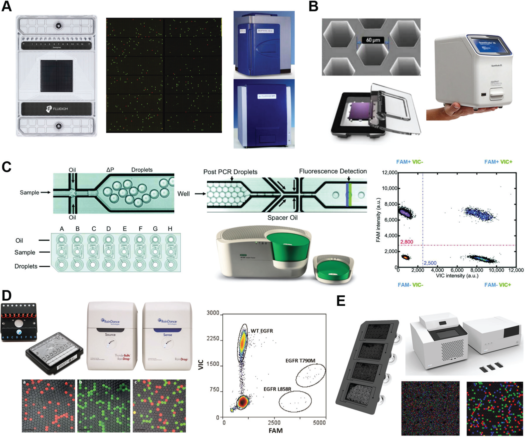
Commercial dPCR systems. (
Comparison of Commercial dPCR Systems.
The second category, ddPCR systems, performs PCRs in water-in-oil droplet emulsions, as described in the introduction section. The PCR mix in each droplet must also include PCR-compatible surfactants, often proprietary, to stabilize the emulsion and ensure chemical isolation during amplification. 22 The first report of ddPCR in 2007 49 demonstrated single-copy detection limits using Taqman hydrolysis probes in 10 pL droplets within 18 cycles. This technology was spun out from Lawrence Livermore Labs into QuantaLife, a start-up that developed the first commercial ddPCR system and eventually sold it to Bio-Rad. Bio-Rad’s current offering ( Fig. 6C ) is the QX200 ddPCR system, which generates up to 20,000 droplets with volumes of ~1 nL.40,50 Raindance Technology’s Raindrop system ( Fig. 6D ) 51 generates up to 10 million droplets with volumes of 5 pL, utilizing an array of eight parallel drop generators to increase throughput. Raindance was acquired by Bio-Rad in January 2017. The Stilla Naica System for Crystal Digital PCR 52 ( Fig. 6E ) utilizes step emulsion droplet generators,32,53,54 which can be massively parallelized to hundreds of nozzles; however, Stilla’s current product focuses on a moderate number of droplets (30,000) with short workflow times (2 h) and increased readout capabilities (three fluorescence channels). A unique feature of step emulsion generators is that they do not require the flow of oil; hence, in the Stilla system, the oil is preloaded into the Sapphire chip, simplifying operation and reducing potential contamination.
It is evident that compared with cdPCR systems, ddPCR can readily scale to more partitions in a cost-effective manner. As mentioned earlier, increasing the number of partitions provides several benefits: First, adding partitions proportionally increases dynamic range, so a larger range of samples can be accommodated without dilution. Second, it improves the ability to detect rare targets in the presence of similar nucleotide sequences or inhibitors, due to the enrichment effect ( Fig. 2B ). This is helpful in detecting single-nucleotide polymorphisms (SNPs) and other rare alleles in a largely wild-type population, such as circulating tumor DNA (ctDNA) (to be discussed later). Third, it is better at resolving copy number variations (CNVs), particularly when the target concentration is low. 55
The commercial systems also differ in how they monitor fluorescence during PCR, either by fluorescence imaging or laser-induced fluorescence (LIF) cytometry. The former approach is used in the Fluidigm BioMark system, which is unique in that it can measure fluorescence at each partition after each cycle. The BioMark system can therefore operate in qPCR or dPCR mode. Thermo Fisher’s Quantstudio 12K, a predecessor to the Quantstudio 3D, also provides both capabilities. Real-time, intracycle monitoring on all partitions may help to eliminate false positives in dPCR, but limits the maximum number of supported partitions. Quantstudio 3D and Naica 52 also use fluorescent imaging, but perform only a single-endpoint fluorescence measurement upon the conclusion of all cycles. Fluorescence imaging, when extended to a wide field of view, can analyze as many as 1 million droplets simultaneously. 56 The second approach, LIF droplet flow cytometry, 57 is used by the ddPCR systems from Bio-Rad and Raindance, which serially analyze droplet fluorescence using flow cytometers operating at hundreds or thousands of drops per second. LIF can achieve higher sensitivity and dynamic range than imaging, but its serial nature reading requires more time.
Multiplexing capabilities, offered on all systems to varying degrees, are useful for oncology and food analysis, where multiple targets are quantified simultaneously. The QX200, Raindrop, and Quantstudio 3D support two fluorescence channels at nonoverlapping spectral wavelengths, and Naica provides three. One way to increase the number of fluorophores is amplitude multiplexing, where probes of substantially different intensities can be simultaneously used on the same fluorescence channel. 58 In traditional flow cytometry, amplitude multiplexing comes at the expense of dynamic range, but in digital assays the trade-off is less severe because the fluorescence is used only for counting and not for direct analog quantification. The Raindance system claims to multiplex up to 10 different probes by using 5 amplitude multiplexed probes on two fluorescence channels. For example, a 7-plex assay was used to quantify common mutations in oncogenes. 59 Although not officially offered, other systems in principle should also be able to achieve amplitude multiplexing to various degrees.
Comparison of dPCR with qPCR
Since the transformational invention of PCR in 1983, nucleic acid quantitation has evolved from a qualitative technique (PCR + electrophoresis), to semiquantitative (qPCR), and now, with the advent of dPCR, to absolute quantitation. Compared with its most recent predecessor, qPCR, dPCR provides benefits in three areas. 46
Absolute quantitation. The qPCR workflow requires calibration with standard curves because the relationship between Ct and a target concentration can vary by a factor of 1000, depending on many factors: the target sequence, background, PCR chemistry, primer efficiency, probe intensity, and instrument itself. 12 Generating a standard curve requires sample dilutions over a 5 log range, with multiple replicates at each concentration. Aside from being time-consuming, it requires additional sample, and calibration results may vary from lab to lab. Based on statistical analysis, the digital nature of dPCR provides an absolute quantification of target number, independent of the above factors. As a result, dPCR does not require calibration and is more consistent across laboratories and varying assay conditions. 68 While it is calibration-free, precise quantitation with tight confidence intervals requires that the sample concentration fall within the dynamic range to minimize partitioning error; thus, dPCR may still require a titration step when dealing with unknown concentrations. Absolute quantitation makes dPCR well suited for precision diagnostics and for quantifying DNA libraries for next-generation sequencing (NGS).
Precision. Precision is the ability to reproducibly resolve small differences in copy number, and is necessary for studies in CNV and gene expression. In qPCR, since the fluorescence doubles at each cycle, a single assay can typically resolve only a twofold difference in copy number. Better precision, that is, tighter confidence intervals, can be improved by increasing replicates. One study achieved 1.5-fold resolution with 7 replicates and 1.25-fold resolution with 18 replicates. 45 However, increasing replicates requires additional sample with fixed concentration. In dPCR, the desired precision can be achieved by increasing the number of partitions, which reduces partitioning error. ddPCR routinely achieves 1.25-fold resolution and can resolve 1.16-fold resolution. In Hindson’s study of CNV, 7 ddPCR provides much greater precision (coefficient of variation [CV] decreased 37%–86%) than qPCR, and reproducibility is improved by a factor of 7 while providing single-molecule sensitivity.
Detection of rare targets. A hallmark of dPCR is its ability to detect rare mutants by partitioning, which enriches the mutant relative to the wild type. Both qPCR and dPCR can detect single molecules in “clean” single-plex amplifications. However, in qPCR, inhibitors or excess background DNA can impact amplification efficiency and alter the relationship between Ct and target number. 69 This is especially problematic in rare mutant detection (RMD), wherein the DNA within a sample may contain mutant and wild-type alleles that are both amplified during thermal cycling. If in 100-fold excess or more, the wild-type molecule often overwhelms the lower-concentration target by consuming polymerase, nucleotides, and fluorescent probes to the detriment of the lower-concentration target.5,12 In dPCR, partitioning enriches the target from the background ( Fig. 2B ), which improves amplification efficiency and tolerance to inhibitors. Simultaneously, more partitions increase dynamic range, allowing a high-concentration wild type and a low-concentration mutant to be detected in the same run. The same principles apply to rare sequence detection (RSD).70,71 ddPCR systems can resolve rare mutants (RMD) with <1 in 200,000, and RSD at <1 in 1 million.72,73 RMD and RSD are useful in noninvasive diagnostics for detecting circulating DNA from tumors, fetal cells, or viruses.
On the other hand, qPCR still wins in other areas.
Dynamic range. Dynamic range, the range of sample concentration within which a PCR system can perform quantitation, is a significant strength of qPCR; it achieves a range of >9 log versus up to 6 log for dPCR (although 4–5 log is more typical of dPCR). 12 On the low end of the range, qPCR and dPCR can both detect single molecules, as described above; however, on the upper end of the range, the two methods differ. In qPCR, the inverse exponential relationship between Ct and target concentration results in a dynamic range that can be as much as 10 log. In dPCR, the maximum number of quantifiable targets is limited by the number of partitions to ~6n, but <1.5n is typically used to minimize partitioning error. 38 Bio-Rad’s 20,000-droplet system achieves about a 4 log range, but can be extended to 5 log by splitting the sample between eight sample wells run simultaneously on the same chip. Raindance’s system, with 5 million to 10 million droplets, can reach 6 log. 51 If the sample concentration is above the dynamic range, it must be diluted, introducing an additional step into the workflow. As mentioned above, a large dynamic range is useful in rare mutation detection, and for measuring large differences in expression between two genes. 46
Large volume samples. In clinical diagnostics, patient samples, such as serum, can be in the milliliter range. If the instrument’s sample volume is much smaller, subsampling errors may occur, especially at low concentration. It may fail to collect a minimum number of rare nucleic acid targets necessary for quantitation. 12 As a rule of thumb, in order to have 95% confidence, the lower LOD is three molecules in the sample volume. In this regard, qPCR has an advantage because it can typically accommodate large-volume samples (up 200 µL), while dPCR systems have small sample size (20 µL), necessitated by design. In cdPCR, small chambers reduce chip fabrication and reagent costs, and permit a manageable field of view for fluorescent imaging. In ddPCR, rapid drop generation works best at submillimeter-length scales, resulting in drop volumes of nanoliters down to femtoliters. 74 By comparison, qPCR has no such limit, making it better suited for detecting low concentrations in larger sample volumes.
Throughput. Sample throughput is the number of unique samples that can be processed per day. qPCR wins in this regard because samples are not partitioned, and are read during thermal cycling. Commercial qPCR systems can process thousands of samples per workday. 46 By contrast, the dPCR workflow requires both pre-PCR partitioning and post-PCR reads of each well, limiting throughput. For example, when Raindance’s system is set to 10 million partitions, it can process 16 samples per 8 h workday. The Bio-Rad QX200 system, with only 20,000 partitions, can perform ~96 samples in 5 h. The Stilla Naica System processes 12 samples in <2 h: 15 min to generate drops, 60 min to amplify, and 15 min to read. While dPCR may have higher precision than a single qPCR assay, Weaver et al. argue that qPCR can obtain similar precision by running replicates, and still achieve higher throughput. 45 In laboratory environments where many similar samples are processed with a fixed method and a single calibration, qPCR is more suitable.
Other aspects of qPCR and dPCR systems to consider include the following:
Sample recovery. The recovery of PCR amplified samples is of interest when preparing DNA for NGS. Global recovery of sample is provided by both qPCR and dPCR systems, by either pipetting or breaking the droplet emulsion. 40 However, the recovery of specific partitions in dPCR is not yet available in commercial systems. In principle, it can be done in cdPCR systems by pipetting sample from positive chambers, or in ddPCR systems by sorting droplets of interest using fluorescence-activated droplet sorting. 57
Ease of use. Arguments can be made for both methods in terms of ease of use. Laboratories are more familiar with qPCR, but dPCR does not require calibration, making it more amenable to automation or lay operation. Absolute quantitation also makes it easier for laboratories to reproduce results. However, the lower dynamic range of dPCR means that samples may require predilution. The high throughput of qPCR is more appropriate in laboratory applications where many assays are conducted with a single calibration step, while dPCR may be more simple to use when absolute quantitation is needed on dissimilar samples.
Cost. Considering both capital and per sample reagent costs, dPCR is currently more expensive than qPCR. For example, the Bio-Rad ddPCR system (drop generator, PCR cycler, and reader) costs $90K–$100K, and the reagent cost per sample is ~$5. 60 By comparison, qPCR instruments are in the $25K–$50K range, and the reagent cost is $2. However, the per sample cost in qPCR may be offset by the added costs of calibration standards, whereas dPCR is calibration-free. Given that commercial dPCR instruments have only been available for <10 years, it is expected that their cost will come down over time.
Applications of Digital PCR
Based on the comparisons above, dPCR is best suited in applications where the key requirements are precise and accurate quantification and the ability to detect rare mutants or sequences. On the other hand, qPCR is preferable when dynamic range or throughput is the driver. Examples of dPCR applications ( Fig. 7 ) include CNV for genotyping genetic diversity and disease processes, detection of ctDNA, quantification of viral load and low-level pathogens, and quantification of NGS libraries. Each is discussed in turn below.
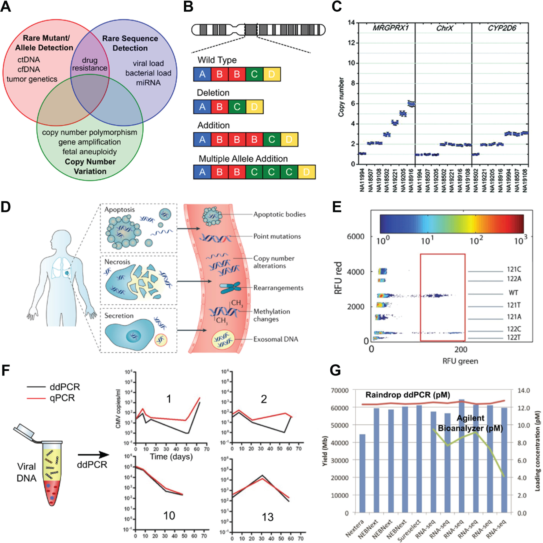
Applications of dPCR. (
Copy Number Variation Genotyping
CNVs (
Fig. 7B
) are sequences of >1 kb pairs that are present in variable copies in as much as 6%–19% of the human genome,75–77 as well as plants.
78
CNVs are considered structural alterations of the genome, and may include the deletion or addition of entire genes, along with their regulatory regions. A rich source of genetic diversity among individuals, CNVs can alter gene dosage, modify protein coding regions, unmask recessive alleles, and influence a variety of complex disease phenotypes,
75
including susceptibility to HIV, autism, and schizophrenia, as well as the process of cancer metastasis.
79
For example, fewer copies of the CCL3L1 chemokine gene can make an individual more susceptible to HIV,
80
but extra copies of the EGFR gene can lead to increased risk for breast cancer.
81
CNV analysis requires quantifying the ratio of a target nucleotide sequence compared with a reference. The first reports of human CNV analysis in 2004 utilized comparative genomic hybridization and complementary microarrays,82,83 and later, sequencing and qPCR provided more quantitative capabilities. Like qPCR, dPCR can quantify CNV in hours rather than days (vs. sequencing), but its advantage over qPCR is its ability to resolve small differences in copy number. Where qPCR can statistically resolve twofold differences (zero to two copies), and with replicates 1.25-fold (up to four copies),
45
a single dPCR run can resolve CNVs up to eight copies. Increasing partition numbers to 1 million or more improves resolution to 1.1-fold differences even in low concentrations (
Fluidigm’s BioMark system (N = 768) was the first commercial dPCR system to report CNV studies in 2008, demonstrating 15% resolution of RPP30 spiked in two haploid genomes. 86 To avoid tandem copies, the authors opted for specific target amplification (STA) instead of restriction enzymes. Prior to dPCR, the target was preamplified together with a reference gene (RNase P) for five cycles, producing separated amplicons at the same ratio as the original sample. STA avoids the stochastic nature of restriction enzymes, but has the potential to introduce bias during the preamplification. In 2011, the Bio-Rad system (N = 20,000) demonstrated precise CNV analysis of up to six copies of MRGPRX1 in HapMap samples 6 ( Fig. 7C ). The same system has been used to measure copy number amplification of HER2 in breast cancer samples.87,88 The more recent Quantstudio 3D system demonstrated a resolution of up to eight copies with <2.6% CV in samples spiked with a known copy number of CCL3L1, and 7% CV for the HER2 gene in breast cancer clinical samples. 89 Using a combination of sequencing and dPCR, Ni et al. provided early evidence that CNVs in circulating tumor cells are specific to cancer types and reproducible among patients, and are thought to play a role in metastasis. 79 Copy number assays also have applications in prenatal screens for fetal aneupoloidy. 90 Trisomy is typically diagnosed by cytogenetic karyotyping of chromosomes obtained from amniocentesis or chorionic villus samples; however, the test can take as much as 1–2 weeks. Using the Fluidigm digital array chip, Fan et al. accurately identified all cases of trisomy in samples within hours. The high-copy-number precision of dPCR is well suited to detecting a 1.5-fold change associated with trisomy. 90
Liquid Biopsy: Detecting Circulating Tumor DNA
dPCR can be used for liquid biopsy, 91 a cancer diagnostic that measures ctDNA released into a patient’s bloodstream by tumor apoptosis, necrosis, or secretion 92 ( Fig. 7D ). Less invasive than direct biopsy, liquid biopsy is particularly attractive when the tumor is not accessible. Several somatic mutations in ctDNA (KRAS, BRAF, NRAS, TP53, PIK3CA, etc.) represent a new generation of cancer biomarkers that can predict, for example, the progression of metastatic tumors 93 , a melanoma’s response to therapies, 94 or a colorectal tumor’s resistance to chemotherapy drugs.93,95 For example, a wide-ranging study by Bettegowda et al. 93 demonstrated the clinical utility of ctDNA in monitoring the progress and even potential morbidity of a variety of cancers. They found that the fraction of patients that had detectable levels of ctDNA increased depending on the stage of cancer: 47% of patients with stage I cancer, and 55%, 69%, and 82% of patients with stage II, III, and IV cancers, respectively. The concentration of ctDNA also increased with stage, and those with lower blood levels of ctDNA lived significantly longer than those with higher levels. The authors concluded that the clinical utility of ctDNA could only be determined by longitudinal studies, necessitating a convenient and sensitive method for liquid biopsy.
A challenge in liquid biopsy is that ctDNA is typically <1% of fragmented DNA in the bloodstream. 71 Moreover, only a fraction of the ctDNA (<10%) is mutated, depending on how advanced the cancer may be. 71 A hallmark of dPCR is its ability to detect rare mutants by partitioning, which enriches the mutant relative to the wild type. ddPCR systems from Raindance and Bio-Rad can resolve rare mutants (RMD) at frequencies as low as 0.0005%,72,73 compared with 1% for qPCR and 2% for NGS. 91 Furthermore, while NGS can only detect if a mutation is present, dPCR can quantify it as well, enabling one to monitor the progression of the disease. When measuring ctDNA, the fact that tumor DNA is as little as 5% makes it proportionally more challenging to resolve subtle changes. The high-copy-number resolution of dPCR (as little as 1.1) is an added benefit in diagnostics that require longitudinal monitoring, such as viral load.
Several studies have shown promising results, beginning with a clinical breast cancer study that detected ctDNA using the Fluidigm BioMark system. 96 The prevalence of the PIK3CA and TP53 loci was shown to be a better predictor of tumor burden than counting circulating tumor cells or conducting an immunoassay for cancer antigen CA15-3. Using a variant of the Raindance system, Taly et al.59,73 devised a multiplex ddPCR method to detect mutations in the KRAS oncogene in patients with colorectal cancer ( Fig. 7E ). Using amplitude multiplexing, they were able to detect up to five mutations in a single experiment, 97 and achieved an RMD sensitivity of 0.0005% (1 in 200,000). Endoplasmic growth factor (EGFR)–activating mutations make the tumor more susceptible to therapies based on tyrosine kinase inhibitors (TKIs).64,65 Stilla’s Crystal Digital PCR64,65 system was shown to detect 3 EGFR mutations involved in TKI susceptibility, all at a frequency of 0.05% compared with the wild-type population.64,65 Oxnard’s study of lung cancer patients 98 used the Bio-Rad QX100 system to regularly monitor EGFR mutations during targeted tumor therapy. Quantitation of EGFR T790M, with a sensitivity of 0.005%, predicted whether the tumor would be susceptible to the targeted drug (erlotinib) or develop resistance to it. Moreover, the mutations were detected up to 16 weeks before tumor growth could be observed via radiometry. These studies show the promise of dPCR in early diagnostics and in guiding therapeutic treatments.
Infectious Disease: Rare Sequence Quantification of Viral or Bacterial Load
Precise quantification of circulating viral or bacterial DNA is critical not only for early diagnosis, but also to monitor the progression of infection and response to treatment. 99 HIV patients undergoing retroviral therapy are regularly monitored for residual infection, and immunosuppressed organ transplant patients are proactively screened for cytomegalovirus (CMV), Epstein–Barr virus, adenovirus, and others. Early diagnostic approaches for identifying pathogens relied on light microscopy; however, this approach was laborious and could not identify small cells like viruses. Since the 1990s, the gold standard has become qPCR, which quantifies viral or bacterial load by measuring circulating DNA. However, in qPCR, the construction of calibration curves and amplification efficiency can vary greatly from lab to lab, resulting in as much as 20%–30% CV at low template concentrations. 99 dPCR provides (1) absolute quantification of target sequences, (2) in some cases, lower CVs at low concentration, and (3) tolerance to PCR inhibitors like sodium dodecyl sulfate (SDS) and heparin.69,100 Sedlak and Gerome’s 2013 and 2014 reviews99,100 outline the use of dPCR in viral and microbial diagnostics, including the measurement of occult RNA, HIV-1, and adenovirus using commercial dPCR products.
In 2008, an early variant of the Raindance platform was used to amplify and detect spiked-in adenovirus solutions with a LOD as low as 1 template per 167 droplets, or 92 per microliter. 101 This chip used continuous-flow ddPCR where droplets shuttle between hot and cold zones during amplification, and cross “neck-down” regions where their fluorescence is detected. In 2013, Strain et al. 102 used the Bio-Rad QX100 system to quantify HIV pol and 2-LTR circles in more than 150 clinical blood samples. For HIV pol, they determined that ddPCR was 5× more precise than qPCR for template frequencies less than 300 copies per million cells. The ddPCR LOD, determined by subsampling error, was 14 copies per million cells (95% CI). However, the dynamic range of 105 required that the sample be diluted to accommodate the high amount of normalization gene. Two studies compared the QX100 ddPCR system with qPCR in measuring CMV spiked in clinical samples.103,104 While Hayden et al.’s initial study suggested that dPCR had less sensitivity and precision than qPCR in clinical samples, 104 Sedlak’s subsequent report showed that with equal sample volumes, ddPCR achieved the same sensitivity and better precision at loads of >104 IU/mL. 103 The authors also demonstrated longitudinal CMV monitoring in a patient population ( Fig. 7F ). On a broader note, although dPCR did improve precision, it did not ultimately improve clinical outcomes, and therefore, with its lower throughput and higher costs, replacing qPCR may not yet be justified. 103 Looking ahead, one of the challenges in virology is quantitation at near- or subtherapeutic thresholds. Currently, qPCR can detect 40–60 copies/mL, but cannot quantitate it. 103 For dPCR to provide precision at such low concentrations would require that the sample be preconcentrated to reduce subsampling error. A second opportunity is quantitation of viral standards. With its ability to perform absolute quantitation, ddPCR systems (Bio-Rad and Raindance) are more suitable than qPCR when validating CMV standards sold by commercial sources. 105 Lastly, as noted by Sedlak, the role of dPCR in viral diagnostics may include the detection of not only viral sequences, but also their mutations, which lead to antiviral drug resistance. 99 Such a capability would require rare sequence, as well as rare mutant, detection ( Fig. 7A ).
Quantitation and Preamplification of Next-Generation Sequencing Libraries
NGS begins with a high-quality DNA library in precise quantities. Constructing an NGS library (e.g., Illumina) includes several steps: fragmentation of the genomic sample, size selection, end repair, adapter ligation, PCR enrichment, and quantitation. Of these, dPCR has proved to be useful in evaluating the integrity of size selection, enrichment, and quantitation. Using the Raindance system, Didelot et al. 106 used ddPCR to quantify the size distribution and integrity of DNA fragments. They performed multiplex ddPCR with four primer probes, each targeted to different lengths of DNA. In doing so, the approximate distribution of nucleotide sequence lengths could be digitally quantified by counting the number of amplified species resulting from each probe. When the same distribution is analyzed using qPCR, it has CVs on the order of 10%–50%. After library construction, a portion of the genomic sample is selected for sequencing. Targeted sequencing often requires unbiased amplification of predesignated loci, usually by PCR with a selected primer library. The common issue of biased amplification can be addressed by dPCR. Partitioning fragmented DNA into small containers effectively enriches the target sequences against background, thus improving the amplification of rare sequences or those difficult to amplify. Using a variant of the Raindance system, Tewhey et al. 107 amplified nearly 4000 targets simultaneously using a highly multiplexed primer library. First, multiple droplet libraries containing each of the primers were generated and pooled. Then, the primer library drops were serially merged with droplets containing the genomic sample. After PCR, the droplet emulsion was broken, and the amplified DNA was enriched and sequenced with high specificity and sensitivity. The last but important use of dPCR is quantitation. To achieve high-yield and high-quality sequencing, NGS sequencers require a relatively narrow range of DNA loading capacity (e.g., Illumina suggests 60 gigabases per lane 108 ). Too little DNA will result in poor coverage, low read depth, and failure to detect SNPs or rare sequences. Too much will result in overclustering, where all sequences may not be resolved. DNA quantitation with spectrophotometry or fluorescence is qualitative and has limited sensitivity, requiring more than 1000× more sample than the sequencer itself, and thus wasting precious sample. 109 Using the Fluidigm dPCR chip with universal adapter primers, White et al. demonstrated absolute quantitation of as few as 100 template molecules, and was able to sequence with nanogram-scale libraries rather than microgram ones. 109 In another example, quantitation by the Raindance ddPCR system correlated more closely with sequencing yield compared than the Agilent Bioanalyzer, which uses capillary electrophoresis and fluorescence 108 ( Fig. 7G ). In this study, 11 samples were sequenced using an Illumina HiSeq 2500. Prior to loading, the DNA was quantified using both methods, and 60 GB was loaded onto each lane based on the ddPCR quantitation. The ddPCR provides more accurate and precise quantitation, which correlates more closely to yield than the Bioanalyzer; however, it should be noted that the Bioanalyzer also provides sizing data. Postsequencing, ddPCR can be used to validate any discovered target sequences. Due to the excellent quantitation and amplification capabilities of dPCR, it is rapidly becoming a standard tool in NGS.
Quantifying mRNA through Reverse Transcriptase dPCR
By adding a reverse transcription step, dPCR can quantify RNA levels with virtually all the benefits of digital partitioning. Of particular interest is the detection of circulating microRNAs (miRNAs), which are known to be biomarkers for cancer, endocrine dysfunction, and other diseases. 7 Hindson et al. demonstrated reverse transcriptase (RT) dPCR by performing a reverse transcription step manually prior to dPCR in the Bio-Rad QX100 system. 7 RT-dPCR had 37%–86% lower variability and 7× better day-to-day reproducibility than its qPCR counterpart, and with a similar detection limit. In serum samples, RT-dPCR could better distinguish between samples that were positive or negative for miR-141, a prostate cancer marker. Similar studies have validated plasma miRNA biomarkers for lung 110 and breast cancer. 111 Intracellular RNA profiling of single cells was demonstrated by Warren et al., using the Fluidigm digital array chip (N = 1200). 112 Harvested cells were stained and sorted by fluorescence-activated cell sorting (FACS) before being individually lysed and transferred to the chip. Their study investigated gene expression in five types of hematopoietic precursors, revealing heterogeneous expression of PU.1 and GADPH, housekeeping genes previously thought to remain constant. Gene expression studies with RT-dPCR offer absolute quantitation of mRNA even at the single-cell level. Higher-throughput alternatives to RT-dPCR now include recent methods for single-cell transcriptome sequencing, 113 to be covered in Part II of this review. Lastly, RT-dPCR has also been applied to viral monitoring of GBV-C, an occult RNA virus that can slow the progression of HIV.99,114 After total cell RNA isolation and reverse transcription, White et al. used the Fluidigm 48.770 chip (N = 770) for dPCR, demonstrating 11% variability compared with 23% for qPCR, and a LOD of 3–10 copies/µL, lower than that for qPCR.
Food and Agricultural Testing
dPCR has also found use in the testing of environmental samples (seeds, plant material, soil, and wastewater), where inhibitors from the DNA isolation process can decrease the efficiency and reproducibility of qPCR. 115 Morisset et al. 116 demonstrated the utility of ddPCR for quantifying genetically modified organisms (GMOs) in maize feed samples. 117 A duplex ddPCR assay compared levels of the MON810 transgene with those of the HMG reference gene. The assay achieved a sensitivity of five target DNA copies and a wide dynamic range, similar to that of qPCR, and reported better repeatability and better tolerance to seed powder inhibitors than qPCR. dPCR has been used to quantify pathogenic bacteria in plants, 118 and Rački et al. used RT-dPCR to detect pepper mild mottle virus and showed it was more tolerant to complex matrices and inhibitors than qPCR. 115
Summary and Conclusions: Part I
Digital assays partition samples into thousands of wells or droplets, and utilize Poisson statistics to calculate the sample concentration with absolute precision. The most mature digital assay is dPCR, evidenced by several commercial instruments currently used by researchers for a wide variety of applications. With the advent of dPCR, nucleic acid amplification has evolved from qualitative (PCR + electrophoresis) to semiquantitative (qPCR), and now to absolute quantitation. dPCR substantially improves precision in counting single molecules and resolving a small number of copies in the presence of inhibitors or wild-type populations. However, it does so at the expense of throughput. The applications of dPCR center primarily around three key capabilities: rare mutation detection (ctDNA), RSD (viral load, bacterial load, and circulating miRNA), and precise copy number quantitation (CNV and NGS libraries). Looking to the future, the use of dPCR in quantifying circulating nucleic acids is gaining widespread acceptance and holds considerable promise in improving detection limits and lab-to-lab reproducibility. To further standardize methodologies and results, Huggett et al. published the dMIQE (Minimum Information for Publication of Quantitative Digital PCR Experiments). 41 The use of dPCR is also quickly becoming a standard technique in NGS library prep. 109 Having covered digital assays with nucleic acids on Part I of this review, Part II will focus on digital approaches in proteins and cells.
Footnotes
Acknowledgements
The author thanks Dr. Rémi Dangla for insightful comments and discussions on the manuscript, and Priyan Weerappuli for a detailed manuscript review.
Declaration of Conflicting Interests
The author declared no potential conflicts of interest with respect to the research, authorship, and/or publication of this article.
Funding
The author disclosed receipt of the following financial support for the research, authorship, and/or publication of this article: The author gratefully acknowledges support from the National Science Foundation Division of Chemical, Bioengineering, Environmental, and Transport Systems (CBET), award numbers 1236764 and 1512544, and from the Division of Electrical, Communications and Cyber Systems (ECCS), award number 1232226.