Sage Journals: Discover world-class research

Abstract

The assay metric Z’ has come to play a critical gatekeeping role in determining whether high-throughput assays can be performed. While Z’ is commonly required to be > 0.5, this expectation is not well supported. Requiring Z’ > 0.5 likely prevents many potentially useful phenotypic and cell-based screens from being conducted, and causes other assays to be conducted under extreme conditions that may prevent activity from being found. We used power analysis and a novel numerical simulation approach to determine how Z’ reflects assay performance under a variety of conditions. Our results show that assays with Z’ > 0.5 perform better than assays with lower Z’, but when an appropriate threshold is selected, assays with Z’ < 0.5 can almost always find useful compounds without generating too many false positives. We provide a method that will allow researchers to estimate how to set an appropriate threshold for their assay. We suggest that instead of always requiring Z’ > 0.5, assays with Z’ < 0.5 should be performed when they can be justified in terms of the importance of the target and the limitations of alternate assay formats.

Keywords

cell-based assays phenotypic drug discovery assay development screening metrics

Introduction

The assay quality metric Z’ was introduced in 1999 by Zhang et al.¹ in a paper that has so far been cited almost 6000 times. Z’ is defined as:

1 - \frac{3 * (σ_{p c} + σ_{n c})}{| μ_{p c} - μ_{n c} |}

(1)

where σ and µ represent the standard deviation and mean, respectively. Z’ defines a separation band between normalized positive (pc) and negative control (nc) populations, and unlike other measures of assay quality such as the signal-to-noise and signal-to-background ratios, it takes into account not only the amplitude of responses but also their variance.

Z’ has come to exert a very prominent role in determining whether assays are considered suitable for high-throughput screening (HTS). Despite the fact that there is no direct relationship between Z’ and the probability of correctly declaring a compound a hit,² it is now essentially a universal requirement that for an assay to advance to HTS, Z’ must be > 0.5 (see https://www.europeanleadfactory.eu/how-submit/drug-target-assays/requirements and https://grants.nih.gov/grants/guide/pa-files/par-17-331.html for examples). In the authoritative Assay Guidance Manual, four chapters state that Z’ should be > 0.5 without providing a rationale for the cutoff,^3–6 although two of these^3,6 point out problems that can arise if unrealistically strong controls are used to achieve Z’ > 0.5. A fifth chapter⁷ recommends Z’ > 0.4. This recommendation emerges from two papers; the first defined the ability of an earlier parameter, the signal window (SW), to correctly identify hits,⁸ and the second estimated the relationship between SW and Z’.⁹

Why care if the requirement for Z’ > 0.5 is not firmly rooted in analysis of assay performance? Is it not best to conduct only “excellent” assays? We see two serious negative consequences of rigidly requiring Z’ > 0.5. First, it likely bars many potentially valuable assays from ever advancing to HTS. Cell-based assays are inherently more variable than biochemical assays¹⁰ and therefore may be more likely to have Z’ between 0 and 0.5, as has been noted by Bray et al.³ While target-based screens conducted in vitro with purified proteins have dominated HTS in the recent past, there is a growing sense that drug discovery efforts based on this paradigm have been less successful than anticipated.¹¹ Phenotypic screening, which is an alternative approach, has to be conducted in cells, in organoids, or even in some cases model organisms. It therefore seems likely that requiring Z’ > 0.5 is preventing important and useful phenotypic assays from being done, leaving potentially valuable compounds undiscovered. It is impossible to know how many assays have failed to go forward because of the requirement for Z’ > 0.5, either in assay originators’ labs or during the transition to HTS format in screening centers. We also cannot know how much time has been spent trying to optimize assays unnecessarily to get them to have Z’ > 0.5; our direct experience suggests this might be substantial. Second, and related, the requirement that Z’ be > 0.5 may lead researchers to conduct assays under conditions that maximize Z’ but hinder detection of useful compounds, as has been noted by Glickman⁶ and Bray et al.³ As an example of our experience with this, we recently developed a screen for compounds that act as antagonists of phorbol dibutyrate (PDBU) binding to C1 domains.¹² To achieve Z’ > 0.5, we conducted the screen with a very high concentration (100 nM) of the activator PDBU. Since the Kd for PDBU binding is in the low nM range,¹³ however, we speculate that using PDBU in excess may have prevented us from finding competitive antagonists.

Here, we have explored the effects of Z’ on assay performance using power analysis and a novel computational approach we developed, seeking to determine the practical differences in performance between assays with different Z’ and different distributions of σ. While our results show that assays with Z’ > 0.5 do perform better than assays with Z’ < 0.5, they do not support the use of a strict cutoff based on Z’. Instead, they are consistent with the idea that when an appropriate threshold is chosen, assays with Z’ < 0.5 can have significant ability to detect hits while still generating a manageable number of false positives. We propose that researchers should take a more nuanced approach to using Z’ to assess assay quality, matching threshold selection to assay performance in the context of the unmet need for the assay. Those in a position to determine whether assays are conducted should use these arguments when they make decisions rather than relying on a single metric.

Materials and Methods

For all of our simulations, we used the R software, Version 3.4.4.¹⁴ In our simulations we generated 40,000 compounds so that half were set to be inactive (0% inhibition) and half were simulated to be active. Among the active compounds, 19,800 were generated by drawing random values, x_i, from a geometric distribution with a probability parameter of 0.05. Since this generates positive integers, we transformed these values to y_i = 1−x_i/max(x_i), so that y_i are all between 0 and 1, and they are concentrated very close to 1. The other 200 active compounds were drawn from a standard uniform distribution, to ensure that if we divide the [0,1] segment to 50 bins, there will be a small number of active compounds in every bin. These values were then converted to percent inhibition (% inhibition).

For each Z’ between 0.1 and 0.9 (in increments of 0.1), we calculated the corresponding $σ_{n c}$ and $σ_{p c}$ and introduced Gaussian noise with appropriate σ. We explored two main scenarios. In the first, we assumed constant standard deviation ( $(σ_{n c} / σ_{p c}) = 1 .$ In this case, at any level of activity, σ = $(1 - Z') / 6 .$ In the second, we set the standard deviation to be proportional to the % inhibition, so that the average standard deviation is determined by the assays Z’ and thus is equal to (1 − Z’)/6. For some constant, C, we calculate σ as a function of the % inhibition, p, as follows:

σ (p) = \frac{2 σ_{0}}{C + 1} . (C + \frac{p (1 - C)}{100})

(2)

With this formulation, when C = 1, we get the constant variance case, because $σ (p) = σ_{0}$ for all p. In general, $σ (p)$ is a linear function of p, and $\frac{1}{2} (σ (100) + σ (0)) = σ_{0} .$ For example, for Z’ = 0.4, we get $σ_{0} = 0.1,$ and if C = 5, $σ (0) = 1 / 6$ and $σ (100) = 0.2 / 6 .$ Supplemental Figure 1 shows the values of $σ (p)$ when Z’ = 0.3, for C = 1, 2.5, 5, 10, and ∞, to illustrate the procedure’s output. Note that for C =∞, we define $σ (p) = \frac{2 σ_{0} (100 - p)}{100} .$ For each level of compound activity, we then introduced Gaussian noise using the calculated σ.

Results

Estimating Assay Power When the Standard Deviation Is Constant

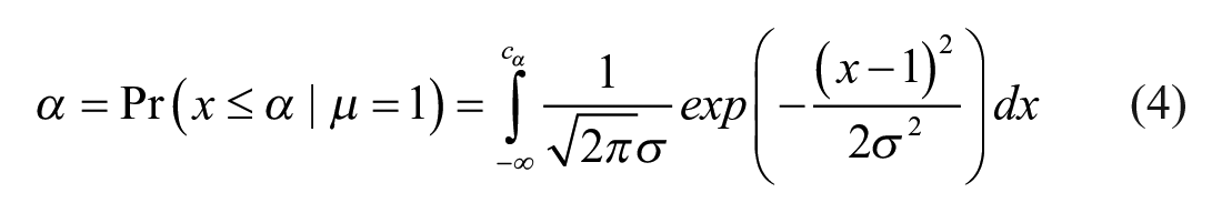
Z’ is a normalized measure that in the simplest case assumes constant σ regardless of response amplitude.¹⁵ Under the conditions of these assumptions, Z’ depends (linearly) on σ alone. One way to assess the effect of Z’ on assay performance is to estimate power (1 − β, where β is the type II error rate), which is the ability to correctly reject the null hypothesis and detect genuine hits. If one sets α, the type I error rate (which is the probability of incorrectly rejecting the null hypothesis, or accepting a false positive), to a desired value, this can be done for different effect sizes and Z’ using Equation (3):

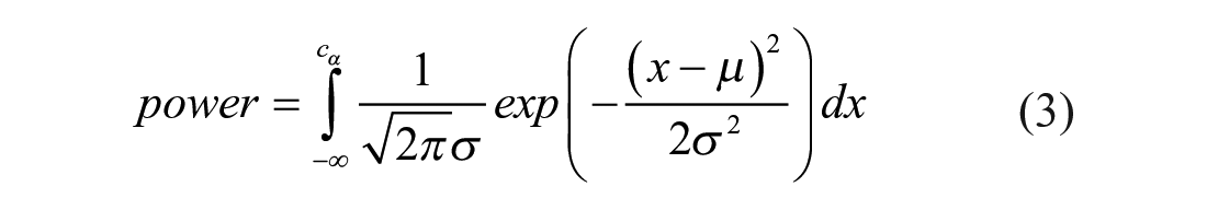
power = \int_{- \infty}^{c_{α}} \frac{1}{\sqrt{2 π} σ} e x p (- \frac{{(x - μ)}^{2}}{2 σ^{2}}) d x

(3)

where $μ < 1$ is the activity under the alternative, and we use the one-sided $c_{α}$ cutoff to control the probability of a Type I error at the α level, under the null hypothesis of no activity [mean = 1; see Equation (4)]

α = \Pr (x \leq α | μ = 1) = \int_{- \infty}^{c_{α}} \frac{1}{\sqrt{2 π} σ} e x p (- \frac{{(x - 1)}^{2}}{2 σ^{2}}) d x

(4)

and σ = (1-Z’)/6 is determined from the Z’ value as described above.

Note that for this and all results described below, we have adopted the convention that we are screening for inhibitors. The exact same logic applies, however, for activator screens. We also multiply power by 100 and report it as a percentage to simplify written descriptions. Figure 1 shows plots of power as a function of Z’ and inhibitory effect calculated for α < 0.05, 0.01, and 0.001 for Z’ ranging from 0 to 0.9. An assay with a Z’ of 1, where σ is 0, would be able to detect any level of inhibition with a power of 1 and a false positive rate of α < 0.05. Such an assay is indeed “ideal” in the sense that it likely cannot be achieved in the real world. The calculations show that for α < 0.05, an assay with Z’ = 0.9 will reach 80% power for levels of inhibition greater than ~4%. As Z’ is decreased in steps of 0.1, the level of inhibition needed to achieve 80% power increases linearly, but by only ~4% per step. An assay with Z’ = 0.5 thus reaches 80% power when compounds inhibit by > ~20%. Assays with Z’ < 0.5 behave surprisingly well by this measure. An assay with Z’ = 0.1 reaches 80% power when inhibition is > ~36%.

Figure 1.

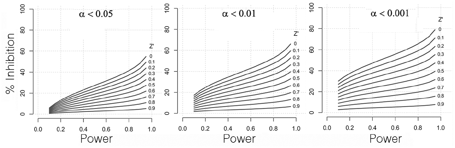
Assays with Z’ < 0.5 have significant statistical power when the standard deviation is constant. Plots of percent inhibition versus power for α < 0.05, 0.01, and 0.001 allow determination of the level of inhibition needed to generate a desired statistical power level.

Because the vast majority of compounds are likely without effect (see below), it is generally accepted that α = 0.05 would result in too many false positives. Higher activity levels are required if either lower α or more power is desired, but assays with Z’ < 0.5 still appear to perform well. For α < 0.001 (which corresponds to the > 3σ assumption that is implicit in the definition of Z’), an assay with Z’ = 0.9 reaches 80% power for compounds that inhibit by > 6.7%. As Z’ decreases in steps of 0.1, the level of inhibition required for 80% power increases, but only in steps of ~6%. Thus, for Z’ = 0.5, inhibition by >32% is required for 80% power, but an assay with Z’ = 0.1 reaches 80% power when inhibition is >58%. To achieve 90% power, these values increase to 35% and 65%, respectively. Assays with higher Z’ clearly perform better by this analysis, but there does not seem to be a compelling rationale for rejecting assays with Z’ below 0.5.

A Novel Approach to Simulating Assay Performance under the Assumption of Constant Standard Deviation

Power analysis is most applicable when trying to distinguish between two normally distributed populations. In terms of screening, those populations would be “active” and “inactive” compounds. In screening, however, compounds can have a range of effects. When analyzing assay performance, what we really would like to know is not just how many active compounds assays with different Z’ will find but also how active those hits are likely to really be, since compounds with low levels of activity may not be any more desirable than completely inactive ones. This is a complex problem depending on both the properties of the assay and the distribution of activities in the compound library being screened, and analytic solutions are impossible. It is possible, however, to solve the problem numerically, provided we try to duplicate what happens in an assay and are willing to make some assumptions about the distribution of activity in the compound library. Taking the assay component first, Z’ is commonly understood as defining a separation band between the positive and negative controls,¹ which it does. The σ we measure when we assess how the sum of all of the errors in the system (liquid handling, compound dispensing, measurement instrumentation, biology, etc.) introduces uncertainty into defined control signals, however, also applies to our estimates of the effects of test compounds throughout the entire signal range of the assay. This means that when we measure the effect of a compound in an assay, we do not obtain the “true” value of its effect (unless our assay has a Z’ of 1 and therefore a σ of 0). Instead, we get a noisy estimate; the “true” effect of a given compound lies probabilistically within a normal distribution (whose width is defined by σ) that includes the measured value. Turning to the compound library, the number of both active compounds found and false positives generated obviously depends on the distribution of compound activities in the collection being screened. There can be no genuine hits in a library with no active compounds, and there will be no false positives if all compounds are active. Unfortunately, we do not know the true distribution of compound activities for any compound library, because this is always measured in the presence of noise introduced by an assay.

We put these two pieces together as follows to mimic an assay in silico. We first modeled a modestly sized “typical” screening collection composed of 40,000 compounds, assuming that compound activity would be distributed in a more-or-less exponential fashion with fewer and fewer compounds demonstrating progressively higher levels of inhibition. We assigned about half the compounds to have absolutely no inhibitory effect at all, another ~18,000 compounds to inhibit by 25% or less, ~1900 compounds to inhibit between 25% and 50%, and only ~100 compounds to inhibit by > 50%. The final distribution of activities in our model compound collection is shown in two forms in Figure 2A . Then, for Z’ ranging from 0 to 0.9, we took the “true” assigned inhibitory effect of each compound and assigned the compound a second “assayed” value obtained probabilistically from a normal distribution (whose width was determined by the σ associated with that Z’) containing the “true” value. This procedure converts each of the defined bins of activity in Figure 2A into a normal distribution with σ determined by Z’. For bins with hundreds or thousands of compounds, the procedure results in a fairly well-defined probability distribution for the “assayed” values. Because, however, we assumed that there are relatively few compounds producing higher levels of inhibition, the resulting “assayed” distributions were sparse. To circumvent this, we repeated the overall procedure 100 times for each Z’ and averaged the results. The effects of this procedure on the apparent distribution of compound activities in the set is shown in Figure 2B . As Z’ decreases, the apparent distribution changes fairly dramatically, coming to look more and more like a normal distribution centered on 0% inhibition.

Figure 2.

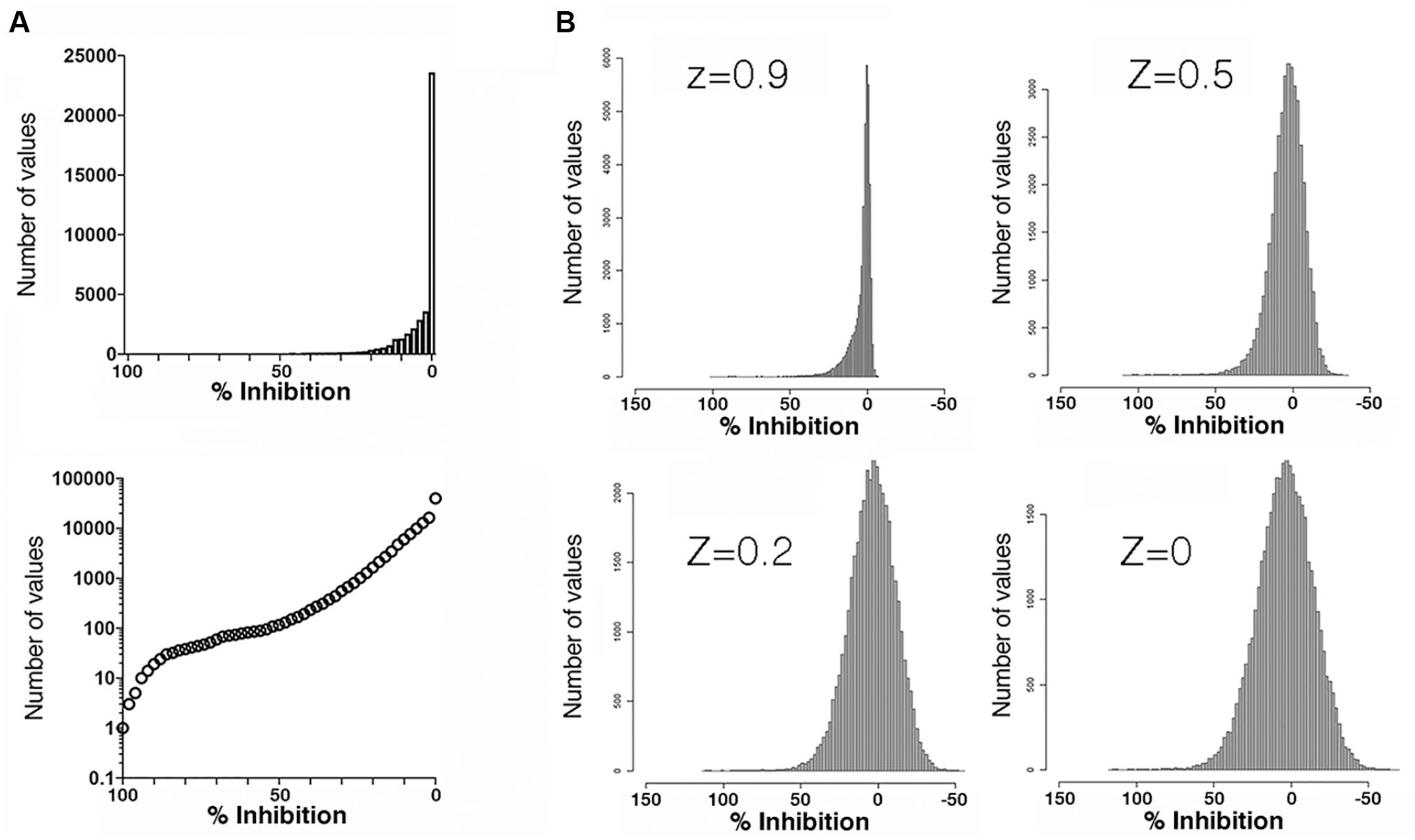
Assay-introduced noise makes a simulated compound collection appear normally distributed. (A) A histogram and a log-scaled cumulative density function display a simulated collection composed of 40,000 compounds. (B) Histograms demonstrate how assays with different Z’ and thus different standard deviations change the apparent distribution of compound activities.

In Figure 3A , we show plots for several different Z’ for three parameters that we calculated as we decreased the observed apparent “assayed” % inhibition from 100%. The first parameter (displayed as a solid line that goes up) is the cumulative total number of apparently active compounds found. Of course, the “true” activity of these compounds may be different than this apparent value. The second (displayed as a dashed line that goes down) is the cumulative number of the 20,000 completely inactive compounds that are mistakenly identified as active as a result of the noise that was added. The final parameter (displayed as a dotted line that goes up) is the cumulative total number of compounds found whose “true” inhibitory activity (i.e., prior to noise addition) is actually ≥ 50%. We included this parameter because it gives us insight as to how assays behave with respect to finding compounds that, while not completely inactive, may be less active than desired. The choice of 50% apparent inhibition was arbitrary but informed by our experience that in many cases, screens are conducted with the intention of finding compounds that inhibit by 50% or more. The utility of this parameter is most readily appreciated in the plot for Z’ = 0 ( Fig. 3A , bottom right). As apparent % inhibition decreases from 100, we initially detect active compounds, almost all of which “truly” inhibit by > 50%, as evidenced by the overlap between the solid and dashed lines. At around 80% inhibition, the curves start to diverge, as we start discovering significant numbers of compounds that “truly” inhibit < 50%, but whose “assayed” values have spread probabilistically so that they falsely appear to produce higher levels of inhibition. By 72% inhibition, only 80% of the compounds that we detect as apparently inhibiting ≥ 50% in fact do so. The other 20% that we thought we found “truly” inhibit less. Since we know how many compounds there are in our set that inhibit ≥ 50%, we can determine that we have found only ~53% of them at this threshold of 72% apparent inhibition. In terms of our 40,000-compound set, this equates to identifying 74 compounds that appear to inhibit ≥ 50% in a primary screen and then having 59 of them confirmed with retesting; 53 compounds that really inhibit ≥ 50% remain undiscovered. We could find more and more of them if we set progressively less stringent thresholds, but then we would mistakenly find relatively more compounds that inhibit < 50% as we went, so our success rate on retesting would decrease. We arbitrarily chose the threshold at which 80% of the compounds identified as inhibiting ≥ 50% actually do so (referred to from here onward as T_80%≥50, as described above = 72% for Z’ = 0) as a means of comparing performance of assays at different Z’. This parameter is not calculated; it is determined analytically based on our knowledge of each compound’s “true” and “assayed” inhibitory activity. For an assay with Z’ = 0.9, T_80%≥50 is 49%, at which point we will have discovered ~99% of all of the compounds that inhibit by ≥ 50%. For an assay with Z’ = 0.5, T_80%≥50 is 53%, at which point 84% of all the compounds that inhibit ≥ 50% will have been found. For an assay with Z’ = 0.1, T_80%≥50 is ~68% inhibition, by which point 58% of the compounds that inhibit by ≥ 50% will have been discovered, which does not seem too bad. Overall, while this analysis indicates that assays with higher Z’ do a better job of finding all of the compounds that we want to find, it also demonstrates that if an appropriate threshold is selected, assays with Z’ < 0.5 are still capable of finding many useful compounds without also identifying an overwhelming number of less active compounds that will need to be retested and discarded. Values for T_80%≥50 and the total fraction found of compounds that inhibit ≥ 50% for different Z’ are presented in Table 1 in the column labeled $σ_{n c} / σ_{p c} = 1 .$

Table 1.

Calculated Performance of Assays with Different Z’.

$σ_{n c} / σ_{p c}$	1		2.5		5		10		∞
Z’	T_80%≥50	Fraction	T_80%≥50	Fraction	T_80%≥50	Fraction	T_80%≥50	Fraction	T_80%≥50	Fraction
0	72.4074	0.526786	81.8769	0.348214	92.007	0.205357	97.953	0.169643	—	—
0.1	66.9019	0.580357	74.3894	0.446429	82.978	0.339286	89.6947	0.241071	—	—
0.2	62.8278	0.642857	66.6817	0.589286	74.7197	0.4375	80.2252	0.375	83.5285	0.321429
0.3	58.7538	0.723214	62.7177	0.625	65.5806	0.589286	70.6456	0.482143	74.7197	0.5
0.4	56.1111	0.767857	58.0931	0.732143	61.0661	0.660714	63.1582	0.607143	73.7287	0.508929
0.5	52.9179	0.839286	54.7898	0.776786	56.992	0.732143	58.4234	0.732143	64.3694	0.651786
0.6	50.6056	0.919643	51.7067	0.875	52.1471	0.839286	53.5786	0.803571	57.5425	0.767857
0.7	48.7337	0.955357	50.1652	0.928571	50.8258	0.919643	49.7247	0.928571	53.3584	0.875
0.8	48.6236	0.964286	49.7247	0.9375	50.0551	0.928571	50.2753	0.928571	52.1471	0.946429
0.9	49.1742	1	49.8348	0.991071	49.9449	0.982143	50.1652	0.982143	50.6056	0.982143

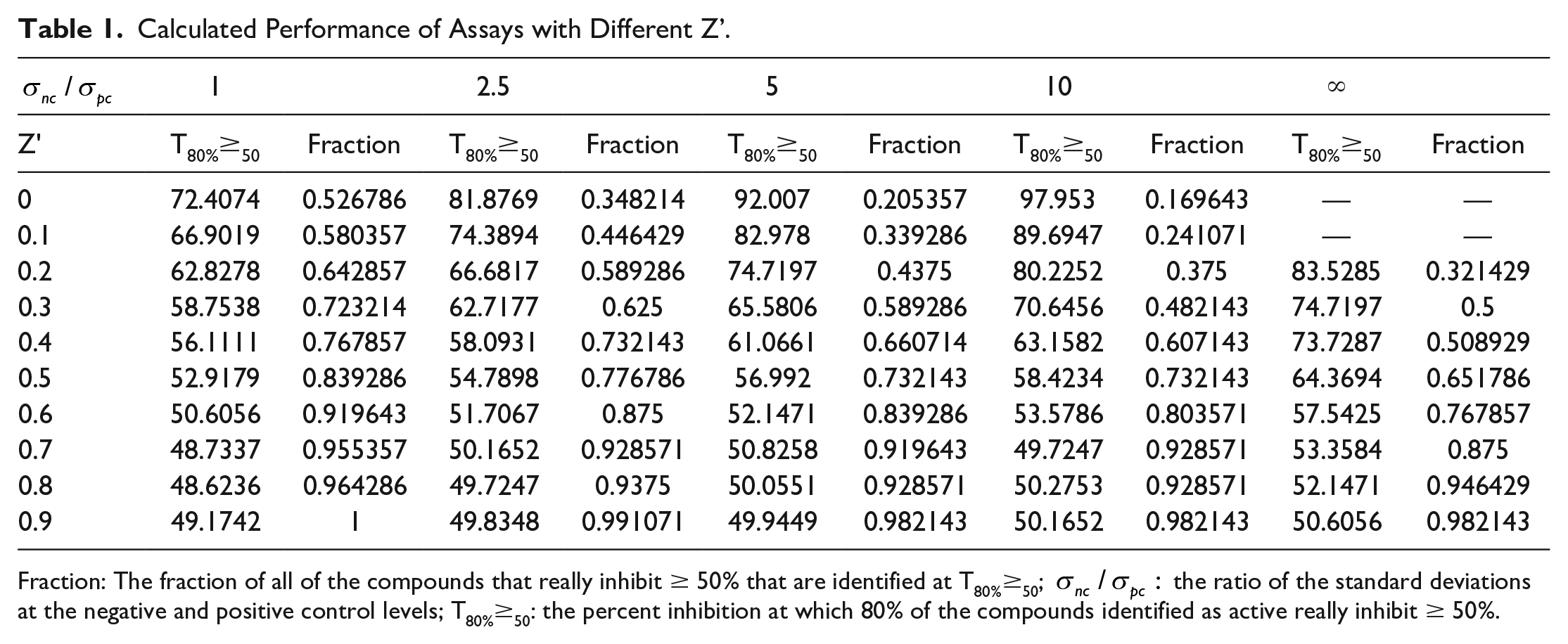
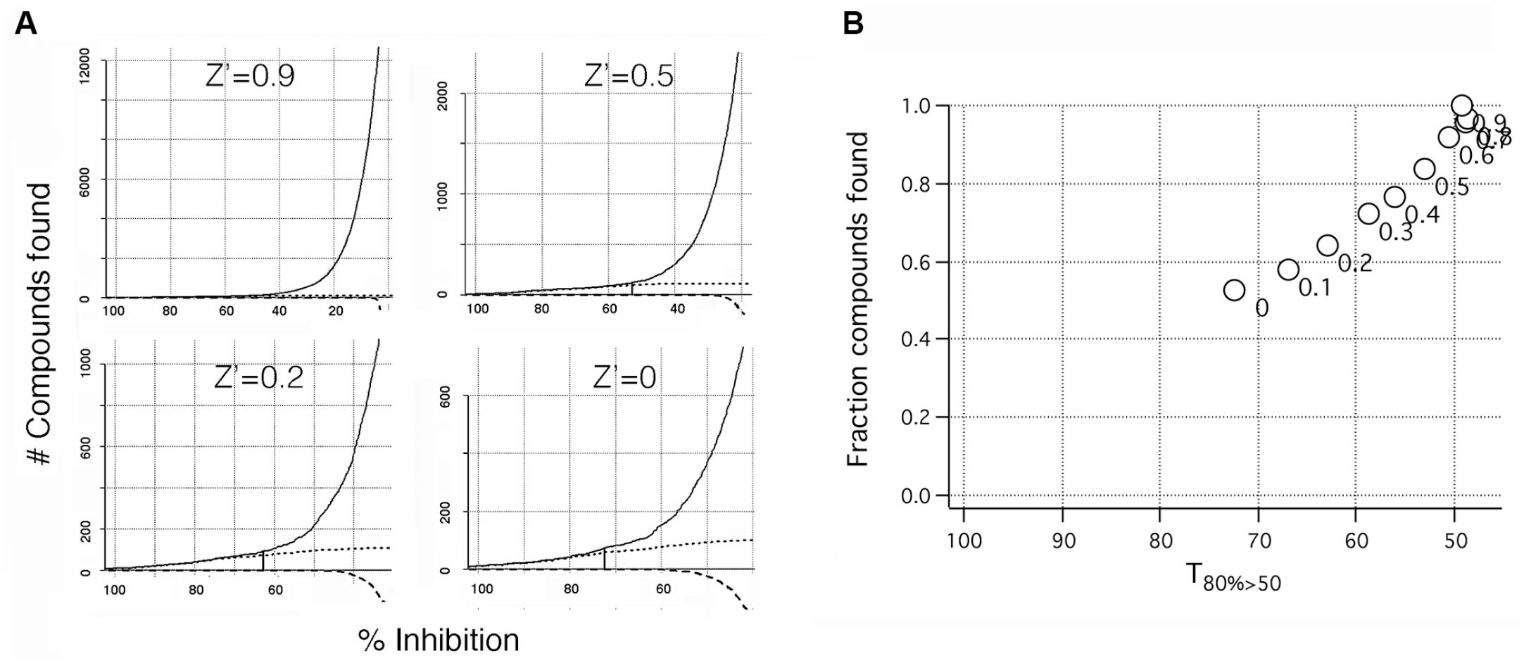
Fraction: The fraction of all of the compounds that really inhibit ≥ 50% that are identified at T_80%≥50; $σ_{n c} / σ_{p c} :$ the ratio of the standard deviations at the negative and positive control levels; T_80%≥50: the percent inhibition at which 80% of the compounds identified as active really inhibit ≥ 50%.

Figure 3.

Simulations indicate assays with Z’ < 0.5 have significant ability to find compounds when the standard deviation is constant. (A) Plots of the total number of compounds found (solid line, upward), the total number of completely inactive compounds misidentified as active (dashed line, downward), and the number of compounds found that actually inhibit ≥ 50% (dotted line, upward) as a function of apparent percent inhibition for the indicated Z’. The vertical lines indicate the percent inhibition at which 80% of the compounds identified as active in fact inhibit ≥ 50%. This parameter, which we call T_80%≥50, is used to characterize assay performance. (B) Plots of the fraction of the compounds that inhibit ≥ 50% found as a function of T_80%≥50 for assays, with the Z’ indicated slightly below and to the right of each symbol.

Assay Performance When the Standard Deviation Is Not Constant

So far, we have considered only assays in which the standard deviation is constant. As Sui and Wu have noted, however, it is often the case that σ varies with signal amplitude, and they demonstrated that this can profoundly affect assay power.¹⁵ To examine how unequal standard deviation affects assay performance, we repeated both our power analysis and our simulations under conditions in which σ increased linearly with signal amplitude from a low value of $σ_{p c}$ (i.e., 100% inhibition) to a high of $σ_{n c},$ so that $σ_{n c} / σ_{p c}$ was 2.5, 5, or 10. We also simulated the most extreme case possible, in which $σ_{p c}$ = 0 and thus $σ_{n c} / σ_{p c}$ = ∞.

Power analysis suggests that unequal σ has relatively small effects when Z’ is > 0.5, but degrades assay performance when Z’ < 0.5 ( Fig. 4A ). As stated above, for α < 0.001, an assay with Z’ = 0.5 reaches 80% power for compounds that inhibit > 32% when $σ_{n c} / σ_{p c} = 1 .$ This increases as $σ_{n c} / σ_{p c}$ increases, reaching a value of ~55% for $σ_{n c} / σ_{p c}$ = ∞. In comparison, when Z’ = 0.1, the percent inhibition required to reach 80% power increases from 58% at $σ_{n c} / σ_{p c}$ = 1 to ~92% when $σ_{n c} / σ_{p c}$ = ∞. Results using the simulation approach also indicate a substantial degradation in assay performance that is particularly pronounced when Z’ < 0.5 (Fig. 4B and Table 1). An assay with Z’ = 0.5 has a T_80%≥50 of 53% and will detect 84% of the compounds that inhibit ≥ 50% when $σ_{n c} / σ_{p c} = 1 .$ When $σ_{n c} / σ_{p c}$ = ∞, T_80%≥50 increases to 65% inhibition and the assay will detect only 65% of the compounds that inhibit >50%. In contrast, an assay with Z’ of 0.1 has T_80%≥50 = 67% and will detect almost 58% of the compounds that inhibit ≥ 50% when $σ_{n c} / σ_{p c} = 1 .$ These values change to a T_80%≥50 = 90% and 24% of total compounds that inhibit > 50% when $σ_{n c} / σ_{p c}$ = 10. When $σ_{n c} / σ_{p c}$ = ∞, there is no T_80%≥50, because at every possible level of inhibition, more than 20% compounds that “truly” inhibit < 50% will be mistakenly found. Of course, the expectation that >80% of the compounds must inhibit ≥ 50% could be relaxed if one were willing to accept the costs of more compounds failing on retest.

Figure 4.

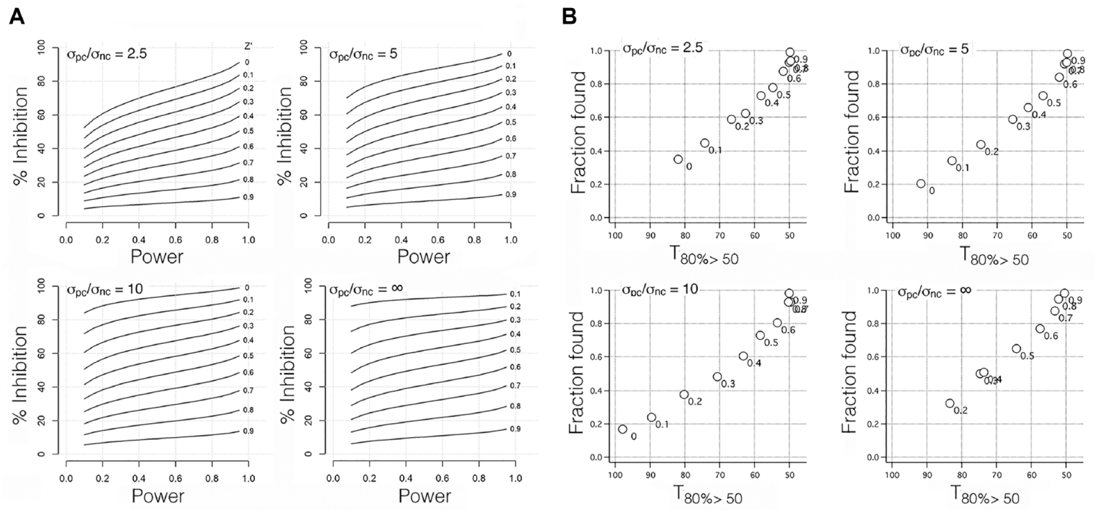
Performance is degraded for assays with Z’ < 0.5 when the standard deviation is not constant, but most assays can still find active compounds. (A) Plots of percent inhibition versus power for assays with $σ_{n c} / σ_{p c}$ indicated. When $σ_{n c} / σ_{p c}$ = ∞, assays with Z’ = 0 have essentially no power at any percent inhibition, so this curve is omitted. (B) Plots of the fraction of the compounds that inhibit ≥ 50% found as a function of T_80%≥50 for different $σ_{n c} / σ_{p c} .$ Z’ to which each symbol corresponds is indicated below and to the right of the symbol. When $σ_{n c} / σ_{p c}$ = ∞, there is no T_80%≥50 for assays with Z’ = 0 and Z’= 0.1 (these will always find > 20% less active compounds), and so the symbols are omitted.

Discussion

Our goal in this work was to determine whether assays should be required to have Z’ > 0.5. We find two compelling reasons why they should not. First, whether assessed by analyzing statistical power or by the simulation approach we developed, it is clear that, except in extreme circumstances, assays with Z’ < 0.5 can find useful compounds without also finding too many unwanted, less active compounds, provided an appropriate activity threshold is selected. Second, Z’ does not serve to allow meaningful comparison of assay performance, assessed either by power calculations or by our simulation method, except when assays have the same $σ_{n c} / σ_{p c},$ and even then it provides no useful information as to how they will perform at finding active compounds. It seems unlikely that Zhang et al. ever intended Z’ to be used as a strict criterion for whether assays should be performed or that they intended Z’ = 0.5 to be used as a cutoff, since they mention having successfully conducted screens with Z’ ranging from 0.2 to 0.6.¹ We suspect that a great deal of confusion was caused by their description of assays with 0 < Z’ < 0.5 as “double” assays, which was a typographical error in the original article (K. Oldenburg, email to A. Zweifach, August, 2, 2018); the intent was to describe these assays as “doable.” Although Iversen et al.⁹ and Sui and Wu¹⁵ correctly deciphered the meaning of this, we speculate that others may not have, and the confusion this caused may have contributed to the idea that Z’ has to be > 0.5.

We have taken two approaches to assess assay performance: power calculations and simulations. Sui and Wu were the first to perform power analysis on assays with different Z’.¹⁵ Our results are largely in agreement with theirs. They found that assuming constant σ and α < 0.001, assays with Z’ as low as 0 retain significant power to find active compounds; for compounds that inhibit by 50%, we both estimate that power = 50%, and show that power increases for compounds that inhibit more than this. Further support for the idea that Z’ need not be > 0.5 can, as mentioned previously, be found by combining the results of two papers from a group at the Lilly Research Laboratories. The first explored the use of the signal window (SW) as an assay quality metric, finding that assays with a SW of 2 or more had reasonable power to identify active compounds.⁸ The second related the SW to Z’, finding that the SW of 2 corresponds to Z’ of ~0.3–0.4.⁹ Sui and Wu¹⁵ also applied power calculations at two signal-to-background ratios when assays have a constant coefficient of variation (i.e., σ is a constant fraction of the signal amplitude). They found that assay performance was substantially degraded. We applied power analysis under four conditions in which σ increases linearly with signal amplitude and also found that assay performance suffers. Except in the most extreme cases, however, our results indicate that power of 80% or more can be achieved if a sufficiently stringent activity threshold is applied.

Our approach to simulating assay performance under different conditions is, to the best of our knowledge, novel. One of the main challenges we faced was deciding on the composition of the model compound collection we used. Zhang et al. mention having assumed a normal distribution of compounds in which the majority have no effect,¹ although it is not clear that this played a significant role in their formulation of Z’. We used a pseudo-exponential distribution instead for the following reasons. It seems to us highly unlikely that in a properly designed screen, equal numbers of compounds will demonstrate blocking and enhancing activity (as we stated, we adopted the formalism of a screen for inhibitors). This would seem to argue against a normal distribution of compound effects. If we were to include enhancing compounds in our set, it would have only minimal effects that would be similar to those of adding additional inactive compounds, but with even less effect on a per-compound basis. Also arguing against an underlying normal distribution of compound activity, we note that the effect of increasing σ in our simulation is to cause the distribution of compound activities to appear progressively more normal. This effect tends to “spread” compound activities to more extreme values. For example, some inactive compounds are made to appear active, an effect that can be appreciated by examining the distribution of compounds for Z’= 0.5 in Figure 2B . Although there are no real enhancing compounds in our set, there appear to be compounds that enhance by more than 30%. Importantly, if the distribution of true compound activities started out as normal and there was any significant width to the distribution, this effect would further spread the values at the extreme of the tails. Since this does not seem to be the case, it suggests that if compounds are normally distributed around 0% inhibition, the width of the distribution must be small and is thus not likely to be a significant factor. We suspect that since the true distribution of activity in a compound library can never be observed, the impression that compound effects are normally distributed is created by the noise introduced by assays. Additional simulation would be needed to determine whether the details of the compound distribution affect results, but because we compared assays using the same set, we suspect any such effect would be small. We note that our simulated set contained ~100 out of 40,000 total compounds that inhibit by > 50%. This would correspond to a hit rate of 0.25% in a screen that set a 50% cutoff for activity, which is reasonable.

A number of assay quality metrics have been proposed that could potentially be used in place of Z’. The group at Lilly Research Laboratories initially proposed the SW,⁸ although they subsequently concluded that Z’ was a better metric.⁹ Zhang² has proposed two parameters—strictly standardized mean difference (SSMD) and coefficient of variability in difference (CVD)—that, unlike Z’, can be interpreted readily in terms of probability of finding active compounds and thus might be better choices than Z’. Sui and Wu¹⁵ suggested replacing Z’ with the power at 50% inhibition. The screening community has so far not adopted any of these alternate metrics, however; acceptance and use of Z’ as an assay quality metric remain widespread in the screening community, and we therefore do not favor replacing it. In fact, we are opposed to using any single assay metric as a strict criterion for assay acceptance. Doing so will continue to cause valuable assays not to be performed and other assays to be performed under non-ideal conditions. As long as important biology is being interrogated, it seems better to us to perform an assay that has a chance of finding some active compounds, even if others will be missed, than not to perform the assay at all and find no compounds. It may also be better in some cases to perform an assay under conditions that yield a lower Z’ than under conditions that give a higher Z’ but may prevent compounds from being found. Our results demonstrate clearly that under almost all conditions at almost any positive Z’, assays can find active compounds without generating too many false positives as long as the threshold selected for defining activity is matched to assay performance.

We recommend the following. Assays with Z’> 0.5 can continue to be justified by this parameter, provided extreme conditions were not used to achieve this benchmark. For assays with Z’ < 0.5, we suggest researchers should use the data in Table 1 to determine the T_80%≥50 for their assay’s Z’ and $σ_{n c} / σ_{p c}$ (which they should calculate in addition to Z’). This will indicate an appropriate threshold to use for hit selection and provide an estimate of the fraction of active compounds they can expect to find. As an example, imagine a researcher who concludes that the best conditions for an assay result in a Z’ of 0.25 and $σ_{n c} / σ_{p c}$ of 7. Although Table 1 does not list values for these conditions, rough interpolation of the values for Z’ = 0.2 and Z’ = 0.3 and $σ_{n c} / σ_{p c}$ = 5 and $σ_{n c} / σ_{p c}$ =10 indicate that if a threshold of 70–75% inhibition is chosen to select hits, ~40–50% of all the compounds that inhibit > 50% will be found, and the use of T_80%≥50 ensures that only 20% of apparent hit compounds will fail to confirm on retesting. We suggest that this information should then be used as part of a detailed justification for the assay that addresses the importance of the target and discusses why the assay should be performed under the conditions chosen, as opposed to other assays or conditions (if such exist) that might yield a higher Z’. Decision makers, rather than relying on a single metric, should in turn be prepared to use the sum total of their expertise, experience, and judgment to assess whether the resulting justification is convincing enough to allow the assay to go forward.

Supplemental Material

Supplemental_Figure_for_Barr_and_Zweifach – Supplemental material for Z’ Does Not Need to Be > 0.5

Supplemental material, Supplemental_Figure_for_Barr_and_Zweifach for Z’ Does Not Need to Be > 0.5 by Haim Bar and Adam Zweifach in SLAS Discovery

Footnotes

Declaration of Conflicting Interests

The authors declared no potential conflicts of interest with respect to the research, authorship, and/or publication of this article.

Funding

The authors received no financial support for the research, authorship, and/or publication of this article.

References

Zhang

J. H.

Chung

T. D.

Oldenburg

K. R.

A Simple Statistical Parameter for Use in Evaluation and Validation of High Throughput Screening Assays. J. Biomol. Screen. 1999, 4, 67–73.

Zhang

X. D.

A Pair of New Statistical Parameters for Quality Control in RNA Interference High-Throughput Screening Assays. Genomics. 2007, 89, 552–561.

Bray

M. A.

Carpenter

Advanced Assay Development Guidelines for Image-Based High Content Screening and Analysis. 2017. In Assay Guidance Manual; Sittampalam

G. S.

Grossman

Brimacombe

, et al., Eds.; Eli Lilly & Company and the National Center for Advancing Translational Sciences: Bethesda (MD), 2004–.

Al-Ali

Blackmore

Bixby

J. L.

, et al. High Content Screening with Primary Neurons. 2013. In Assay Guidance Manual; Sittampalam

G. S.

Grossman

Brimacombe

, et al., Eds.; Eli Lilly & Company and the National Center for Advancing Translational Sciences: Bethesda (MD), 2004–.

Wade

Méndez

Coussens

N. P.

, et al. Inhibition of Protein-Protein Interactions: Cell-Based Assays. 2017. In Assay Guidance Manual; Sittampalam

G. S.

Grossman

Brimacombe

, et al., Eds.; Eli Lilly & Company and the National Center for Advancing Translational Sciences: Bethesda (MD), 2004–.

Glickman

J. F.

Assay Development for Protein Kinase Enzymes. 2012. Assay Guidance Manual; Sittampalam

G. S.

Grossman

Brimacombe

, et al., Eds.; Eli Lilly & Company and the National Center for Advancing Translational Sciences: Bethesda (MD), 2004–.

Iversen

P. W.

Beck

Chen

Y. F.

, et al. HTS Assay Validation. 2012. In Assay Guidance Manual, Sittampalam

G. S.

Grossman

Brimacombe

, et al., Eds.; Eli Lilly & Company and the National Center for Advancing Translational Sciences: Bethesda (MD), 2004–.

Sittampalam

G. S.

Iversen

P. W.

Boadt

J. A.

, et al. Design of Signal Windows in High Throughput Screening Assays for Drug Discovery. J. Biomol. Screen. 1997, 2, 159–169.

Iversen

P. W.

Eastwood

B. J.

Sittampalam

G. S.

, et al. A Comparison of Assay Performance Measures in Screening Assays: Signal Window, Z’ Factor, and Assay Variability Ratio. J. Biomol. Screen. 2006, 11, 247–252.

10.

W. F.

Tolliday

Cell-Based Assays for High-Throughput Screening. Mol. Biotechnol. 2010, 45, 180–186.

11.

Swinney

D. C.

Anthony

How Were New Medicines Discovered?

Nat. Rev. Drug Discov. 2011, 10, 507–519.

12.

Yang

X. A.

Zweifach

Temperature-Dependent Expression of a CFP-YFP FRET Diacylglycerol Sensor Enables Multiple-Read Screening for Compounds That Affect C1 Domains. SLAS Discov. 2019, 24, 682–692.

13.

Das

Rahman

G. M.

C1 Domains: Structure and Ligand-Binding Properties. Chemical Rev. 2014, 114, 12108–12131.

14.

R: A Language and Environment for Statistical Computing. Core Team, R Foundation for Statistical Computing: Vienna, 2018.

15.

Sui

Alternative Statistical Parameter for High-Throughput Screening Assay Quality Assessment. J. Biomol. Screen. 2007, 12, 229–234.

Supplementary Material

Please find the following supplemental material available below.

For Open Access articles published under a Creative Commons License, all supplemental material carries the same license as the article it is associated with.

For non-Open Access articles published, all supplemental material carries a non-exclusive license, and permission requests for re-use of supplemental material or any part of supplemental material shall be sent directly to the copyright owner as specified in the copyright notice associated with the article.

0.00 MB

0.09 MB