Sage Journals: Discover world-class research

Abstract

The Fragile Families Challenge charged participants to predict six outcomes for 4,242 children and their families interviewed in the Fragile Families and Child Wellbeing Study. These outcome variables are grade point average, grit, material hardship, eviction, layoff and job training. The data set provided contained longitudinal survey and observational data collected on families and their children from birth to age 9. The authors used these data to create models to make predictions at age 15. The authors describe the imputation and modeling strategies that led them to make predictions ranked fifth and ninth in the material hardship and layoff categories, respectively. However, the results of the study are inconclusive with respect to increased predictive performance. The authors view this work as a first step toward organizing the Fragile Families missing data by exploiting the structure of the survey instruments.

Keywords

machine learning predictive modeling feature engineering

The Fragile Families Challenge (FFC) was a predictive modeling challenge to identify promising predictors for six measurable outcomes for children and their families. Participants in the FFC were provided data collected from the Fragile Families and Child Wellbeing Study (cf. Reichman et al. 2001; Salganik et al. 2019). This longitudinal data set contains deidentified data for 4,242 children and their families in cities located around the United States. Survey and observational data were collected at the children’s birth, and follow-up studies were conducted at ages 1, 3, 5, 9, and 15, for a total of six collection waves. Using the data from birth to age 9, FFC participants were tasked with creating predictive models for six outcome variables at age 15. The outcome variables were grade point average (GPA), grit, material hardship, layoff, eviction, and job training.

A substantial portion of the work in our submission was the preparation and preprocessing of the data for model training. In this article we discuss semiautomated methods to identify related questions among the survey instruments and use this information to impute missing data. We decided on our approach because we wanted to use the structure of data collection and survey process as much as possible to reason about missing values. Many surveys were conducted, and respondents include parents, teachers, primary caregivers, children, and others. Our primary focus was on surveys administered to the mother and father because these contained relevant responses for household income, relationships, and how time is spent with the child (cf. Reichman et al. 2001). Furthermore, these surveys were administered each collection wave and were the basis for the outcome variables to be predicted. We searched for related questions within individual surveys, between parent surveys, and across collection waves. We found that the results of the effort are inconclusive with respect to predictive performance, but it is a first step in forming a structured approach to imputing missing data in the FFC.

We proceed by first discussing the data set and providing the necessary details to understand our approach. We then discuss our imputation and modeling strategy. We describe the specific types of imputation that were performed on the surveys. Finally, we present the results of our data and modeling work framed in the context of the entire FFC.

Data and Preprocessing

The data in the FFC were split into three categories: training, leaderboard, and holdout data. All of our trials on imputation and model-training operations were performed on the training data set. The remaining data sets were used for intermediate and final model validations. The data from the first five collection waves (birth to age 9) were used as input variables and contained a total 12,942 columns. We refer to these as features. The last wave (age 15) was used as test data for evaluating the model predictions and had six columns of “true” outcomes to be used for comparison. Details of how the outcomes are formed in the challenge are given in Appendix A2. All waves of data contained 4,242 rows, one for each family included in the study.

Missing data were a major obstacle in the FFC. We wanted to have a data set that could be quickly tested with a variety of models, which meant that our specific requirements were to impute all missing data and convert to numeric form. Table 1 shows both the steps taken to impute missing data and the amount of missing data before and after each processing step.

Table 1.

Data and Preprocessing Broken Down by Step.

Step	Name	Number of Features Before and After	Percentage of Data Set Missing Before and After	Number of Features Affected	Number of Rows Affected	Implementation Type
0	Initial preparation	12,942 → 10,423	NA → 54.63	2,519	4,242	—
1	Cross-path imputation	10,423 → 10,423	54.63 → 51.46	1,692	4,242	Automated
2	Cross-caregiver imputation	10,423 → 10,423	51.46 → 45.43	5,169	4,242	Manual
3	Cross-year imputation	10,423 → 10,423	45.43 → 39.33	2,986	4,242	Semiautomated
4	Cross-caregiver imputation (second)	10,423 → 10,423	39.33 → 37.66	1,227	4,242	Manual
5	Mode imputation and and finalization	10,423 → 10,369	37.66 → 0	9,241	4,242	—

Note: This table summarizes each step of the imputation process. The number of features before and after shows how many features were removed during each step. The impact of each step is quantified by the total percentage of missing data imputed. This is further qualified by the number of features imputed and rows affected by each step. Imputation summaries by survey instrument and feature are given in Appendices A7 and A8, respectively.

Step 0: Initial Data Preparation

Two major steps were taken to prepare the data for the subsequent imputation steps. First, all data that could be cast as numeric float values were converted from text to those numeric values. Similarly, categorical (multiple-choice) variables were cast as integer representations when possible. Features that could not be placed into either data type were removed. Second, we removed columns that contained zero variation in the data (were all one value) or were all null valued. As a result of these two operations, 2,519 features were removed from the original training data.

Step 1: Cross-Path Imputation

We refer to a path in the survey as a result of a particular skip pattern. It is a sequence of questions that depends on answers to prior questions or criteria identified during the interview. For example, mothers being surveyed will answer a different set of questions on the basis of their current relationships with their children’s fathers. An inspection of the Fragile Families surveys showed a number of either same or similar questions asked in separate and exclusive paths. This means that a null value appearing for one question in the survey is actually answered in a differently labeled question in the same survey that has either the same or similar question text. For example, in the mother baseline survey, questions B5, B11, and B22, are all the same: “I’m going to read you some things that couples often do together. Tell me which ones you and [baby’s father] did during the last month you were together.” In any given survey, only one of these questions would be answered depending on the path the interview took following these criteria:

questions for mothers who are not romantically involved with baby’s father;

questions for mothers who are in romantic or “on again, off again” relationships; and

questions for married mothers only.

Cross-path imputation is a method to replace question responses that were skipped or not answered by using response values from the same or similar questions elsewhere in the survey but within the same section of questions. This automated algorithm was applied to all surveys, regardless of respondent. Sections of a particular survey are organized to cover major topics such as “income” and “current partner.” Similarity is measured using the Levenshtein edit distance¹ (Bird, Klein, and Looper 2009) between variable labels of survey questions in the same section. These variable labels were encoded by the FFC. Labels with an edit distance of less than 10 were identified and placed into a set. The mean value, in the case of multiple related responses, was then used to replace the original null value. Although a sample of questions were validated by hand and found to be correct, we did observe that there were false positives (see Appendix A3).

Steps 2 and 4: Cross-Caregiver Imputation

In each survey wave (birth, year 1, year 3, etc.), there were a number of same or similar questions when comparing across caregivers. For example, there were questions appearing in the mother survey for a given wave that also appeared in the father survey or the primary caregiver survey. If only one parent was interviewed, the corresponding questions on the other surveys would be null. Two assistants manually identified these questions in each wave. A third person checked the results for validation. Once the related questions were determined, if a question was missing a value, the corresponding survey value was substituted.

Cross-caregiver imputation was performed twice, before and after cross-year imputation. The strategy was to impute within a particular wave in the first iteration of cross-caregiver imputation. The remaining data were imputed after cross-year imputation to capture cases in which only one or no parents would respond after a given wave in the survey.

Step 3: Cross-Year Imputation

Both the mother and father surveys showed monotonic increases in missing values with each successive wave. Although the mother, father, and primary caregiver surveys varied the questions in each wave, there were many similarities. One option was to carry the last completed survey data forward; however, this potentially overrepresents the particular value of the last recorded year, resulting in skewing of the imputed data set. Mode imputation was another option, but we wanted to capture the variation in recorded values across survey waves in the imputation that would otherwise be lost by choosing the most common value. For example, if an eviction was recorded in an earlier survey, we wanted to make sure that it had some influence on the value of the imputed surveys. Although no option is perfect, we chose to take the mean value for a given feature across all of the surveys that were completed. We term this “cross-year” imputation.

Question labels could have different text yet essentially ask for the same information, as shown in Figure 1. The Levenshtein edit distance and simple thresholding produced unreliable matches. Therefore, an algorithm was designed to suggest groups of related questions to a user in each of the survey waves. The algorithm output used the same Levenshtein edit distance from the NLTK toolbox (Bird et al. 2009), and two thresholds were used to identify candidate questions. The first threshold was a hard threshold that determined the preliminary admittance into the set of potential candidates. The user would not see any questions outside of the set. To reduce the chances of false negatives, this primary threshold was set high so that less similar question text would be admitted. However, if the user had to manually remove these entries, that would take more time, which was limited. Therefore, a second lower threshold marked suspect question text with an asterisk. The user need only remove the asterisk for questions that are to be included and put an x next to questions that should not be included. This made it more efficient to scan the sets of question labels and have the user validate. An example of this process is shown in Figure 1. Once completed, the imputation process was conducted sequentially across waves starting with the first two collection waves.

Figure 1.

Two examples of candidate groups of related questions identified by our algorithm. Questions without markers will be clustered, and their values will be averaged to fill in missing data. Questions denoted with an asterisk were labeled as not part of the set automatically, and questions with an x were manually labeled. This procedure was a simple way to find related questions without resorting to much manual effort writing code or comparing surveys.

Step 5: Mode Imputation and Finalization

Our final step was simply to fill in the remaining missing data with most frequent values appearing for a given feature: mode imputation. We did this because most of the input features were interpreted by us to be either categorical or ordinal. This is evidenced by the number of unique values shown in Appendix A4. In retrospect, we would have handled this better by giving different simple imputation assignments to the different continuous or categorical variables. Last, a final pass at removing any columns that displayed zero variation in the data was performed as outlined in step 0.

Feature Engineering

After preparing and imputing the training data set, we created features on the basis of outcome variables using the questions from which they are derived (see Appendix A2). Questions were manually identified and imputed using the steps outlined in Table 1. In addition, grit and material hardship are outcome variables composed of multiple survey questions. The questions that are used to form the grit and material hardship outcomes were summed. This is important because these new features are related to the actual definitions of the outcome variables. For example, material hardship is calculated by taking the average number of “true” responses from 11 binary questions. There is a many-to-one relationship between survey responses and the material hardship outcome that is now captured in these new features.

The last feature-engineering step is to encode integer labels to the categorical data labels. We noticed that many of the survey questions of interest to us had an order to their responses. Therefore, we chose to use the integer labels in some models as continuous input variables. With more time, we would have applied vector (“one-hot”) encoding to truly categorical variables.

Modeling Approach

Model Selection

After completing preprocessing and feature engineering, the result was an imputed set of training data that could be applied to multiple types of models. Because of time and resource constraints, we wanted to quickly test numerous types of models. Therefore, we imposed a self-limited set of models that were easily implementable and available in well-tested packages. We chose the scikit-learn package (Pedregosa et al. 2011) written in Python. With more time, our modeling efforts would have explored relevant social science theories and created heterogeneous models to account for different data types. One model was trained for each outcome variable separately. We experimented with several types of models, both classifiers and regression models. Validating using training data, we found that the linear and logistic regression models tended to perform the best with respect to mean square error (MSE) and were chosen for the final submission. Our final choice of models for the Challenge is listed in Table 2. We found that the L1 regularized linear regression (i.e., least absolute shrinkage and selection operator; Tibshirani 1996) produced the best results using K-fold (10 folds) cross-validation for the GPA, grit, and material hardship outcomes. For the binary variables, eviction, job training, and layoff, we used logistic regression with L1 regularization of the weights.

Table 2.

Summary of Model Selections for Each of the Outcome Variables.

Outcome Variable	Model Type	Number of SelectionK-Folds	Number of Training K-Folds	Number of Features Imputed	Num. Features Engineered	Initial Selection Method
Grade point average	Linear	10	10	28	0	L1-penalty
Grit	Linear	3	10	48	5	L1-penalty
Material hardship	Linear	—	10	41	5	Manual
Eviction	Logistic	—	10	41	5	Manual
Layoff	Logistic	—	10	5	1	Manual
Job training	Logistic	—	10	5	1	Manual

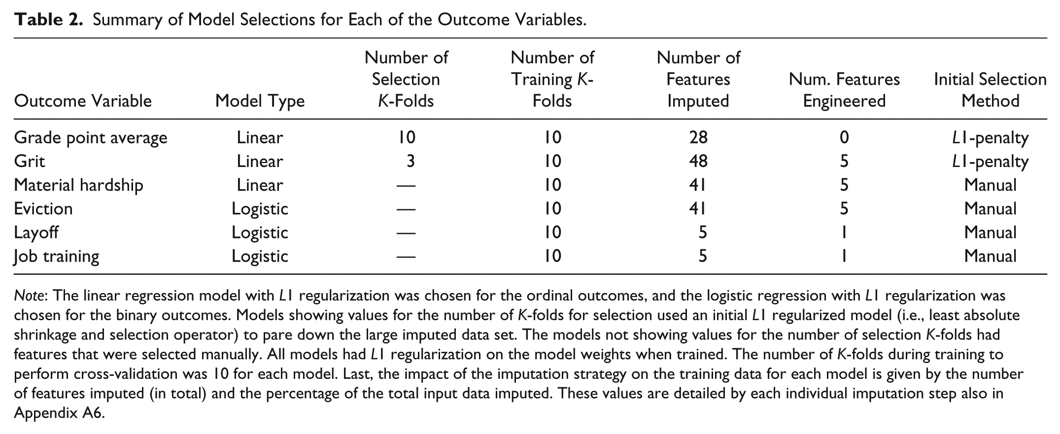
Note: The linear regression model with L1 regularization was chosen for the ordinal outcomes, and the logistic regression with L1 regularization was chosen for the binary outcomes. Models showing values for the number of K-folds for selection used an initial L1 regularized model (i.e., least absolute shrinkage and selection operator) to pare down the large imputed data set. The models not showing values for the number of selection K-folds had features that were selected manually. All models had L1 regularization on the model weights when trained. The number of K-folds during training to perform cross-validation was 10 for each model. Last, the impact of the imputation strategy on the training data for each model is given by the number of features imputed (in total) and the percentage of the total input data imputed. These values are detailed by each individual imputation step also in Appendix A6.

Variable Selection

We used both manual and automated methods for variable selection, as summarized in Table 2. For some outcome variables, we manually identified potentially relevant survey questions and data sources. These manually identified features mostly consisted of the features used to form the outcome variable discussed in the “Feature Engineering” section. If the manually selected subset did not perform well, we used the entire imputed data set for variable selection using L1 regularization. GPA and grit fell into this category. For these models, we selected a subset features that had effectively nonzero weights (i.e., >.00001) in the initial L1 regularized model. A full accounting of the features chosen for each outcome variable is given in Appendix A6.

Challenge Performance Results

The prediction results are summarized in Table 3. Overall, the models in our submission performed better when predicting the material hardship and layoff outcome variables in terms of MSE. These categories both performed better than a mean calculated baseline model and were ranked fifth and ninth, respectively, in the FFC. Distributions comparing our results with the rest of the submissions in the challenge are presented in Appendix A5.

Table 3.

Results of Our Final Submissions Using Both Challenge Ranking and MSE.

Outcome Variable	Outcome Type	Prediction Error	Error Measure	Model Rank	Baseline Error	Model-baseline Improvement (%)
Grade point average	Ordinal	0.365	MSE	36 of 124	0.425	14.04
Grit	Ordinal	0.255	MSE	77 of 111	0.253	−0.96
Material Hardship	Ordinal	0.020	MSE	5 of 113	0.025	21.51
Eviction	Binary	0.055	Brier	33 of 90	0.055	1.07
Layoff	Binary	0.164	Brier	9 of 91	0.167	1.66
Job training	Binary	0.185	Brier	47 of 95	0.185	−0.01

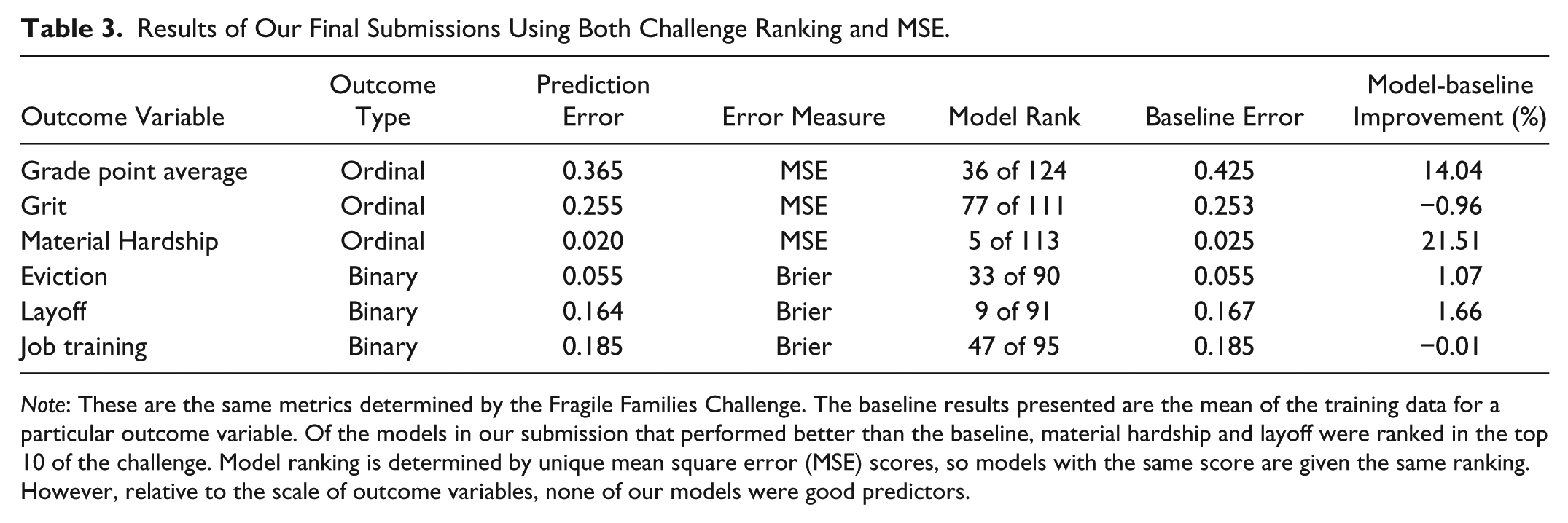
Note: These are the same metrics determined by the Fragile Families Challenge. The baseline results presented are the mean of the training data for a particular outcome variable. Of the models in our submission that performed better than the baseline, material hardship and layoff were ranked in the top 10 of the challenge. Model ranking is determined by unique mean square error (MSE) scores, so models with the same score are given the same ranking. However, relative to the scale of outcome variables, none of our models were good predictors.

Despite FFC rankings, the results of our models and those of the challenge do not indicate particularly predictive models when applied to individual circumstances. This is because error tolerances on individual predictions are not guaranteed with aggregate error measures such as MSE. This is discussed in more detail in Appendix A1. Here, we comment only on the results of our imputation and modeling approach in the context of the challenge. The outcome variables material hardship, layoff, and GPA show improvements over the baseline, and we view this work as a potential first step toward developing imputation techniques for Fragile Families data that exploit the structure of the survey instruments.

Conclusions

In this article we present a submission to the FFC with a focus on the imputation strategy performed. Our approach focused particularly on the structure both within and among the parental surveys. Using a semiautomated process, we imputed data corresponding to related questions within surveys, across survey waves, and across survey respondents. This imputation strategy reduced the total number of missing data from 55 percent to 38 percent before filling the remaining missing values with mode imputation. The results showed mixed performance. Although some models were ranked high in the FFC and several models beat the mean-baseline model, the MSE scores are not likely to show effective model prediction at individual scales (see Appendix A1). The effort described in this article is best characterized as a first step toward organizing and forming model features that exploit the structure of the Fragile Families data.

Supplemental Material

ffc-sage-appendix – Supplemental material for Imputing Data for the Fragile Families Challenge: Identifying Similar Survey Questions with Semiautomated Methods

Supplemental material, ffc-sage-appendix for Imputing Data for the Fragile Families Challenge: Identifying Similar Survey Questions with Semiautomated Methods by Brian J. Goode, Debanjan Datta and Naren Ramakrishnan in Socius

Supplemental Material

SRD-17-0114 – Supplemental material for Imputing Data for the Fragile Families Challenge: Identifying Similar Survey Questions with Semiautomated Methods

Supplemental material, SRD-17-0114 for Imputing Data for the Fragile Families Challenge: Identifying Similar Survey Questions with Semiautomated Methods by Brian J. Goode, Debanjan Datta and Naren Ramakrishnan in Socius

Footnotes

Acknowledgements

We thank Dichelle Dyson and Samantha Dorn. In addition to those already mentioned, the results in this article were created with software written in Python 2.7 using the following packages: Scipy (Jones et al. 2001), Numpy (Oliphant 2006), Pandas (McKinney 2010), Matplotlib (Hunter 2007), and scikit-learn (Pedregosa et al. 2011).

Funding

The author(s) disclosed receipt of the following financial support for the research, authorship, and/or publication of this article: The analysis portion of this research was partially supported by DARPA Cooperative Agreement D17AC00003 (NGS2). Funding for the Fragile Families and Child Wellbeing Study was provided by the Eunice Kennedy Shriver National Institute of Child Health and Human Development through grants R01HD36916, R01HD39135, and R01HD40421 and by a consortium of private foundations, including the Robert Wood Johnson Foundation. Funding for the FFC was provided by the Russell Sage Foundation.

Supplemental Material

Supplemental material for this article is available with the manuscript on the Socius website.

1

The Levenshtein edit distance counts the number of changes needed to be made in one text string to become identical to another.

Author Biographies

Brian J. Goode is a research scientist at the Biocomplexity Institute of Virginia Tech. Brian’s core research interest is developing holistic, quantifiable strategies for bridging the gap between developing models and deployment in terms of policy, decision making, or creating further studies. Brian received his PhD in mechanical engineering with an Office of Naval Research assistantship focusing on differential game control theory to form robust and dynamically evolving strategies. Presently, his research focuses on developing methods to bring more reproducible and replicable research to the social sciences to carry over into the policy and decision space.

Debanjan Datta is a PhD student at the Discovery Analytics Center of Virginia Tech. His research area is data mining, with interests in time series, natural language processing, and general application of machine-learning models to large data sets with practical applications. He was previously a software developer at Yahoo.

Naren Ramakrishnan is the Thomas L. Phillips Professor of Engineering in the Department of Computer Science at Virginia Tech. He is also the director of the Discovery Analytics Center. He received his PhD in computer sciences from Purdue University. His research interests include mining scientific data sets in domains such as systems biology, neuroscience, sustainability, and intelligence analysis. His work has been featured in the National Institutes of Health outreach publication Biomedical Computation Review, the National Science Foundation’s Discoveries series, the Wall Street Journal, Newsweek, Smithsonian, Popular Science, Slate, and ACM TechNews.

References

Bird

Steven

Klein

Ewan

Looper

Edward

. 2009. Natural Language Processing with Python. New York: O’Reilly.

Hunter

John D.

2007. “Matplotlib: A 2D Graphics Environment.” Computing in Science & Engineering 9:90–95.

Jones

Eric

Oliphant

Travis

Peterson

Pearu

et al. 2001. “SciPy: Open Source Scientific Tools for Python.” Retrieved March 16, 2018 (http://www.scipy.org).

McKinney

Wes

. 2010. “Data Structures for Statistical Computing in Python.” Pp. 51–56 in Proceedings of the 9th Python in Science Conference. Retrieved December 23, 2018 (https://conference.scipy.org/proceedings/scipy2010/pdfs/mckinney.pdf).

Oliphant

Travis E.

2006. “A Guide to Numpy.” Trelgol Publishing.

Pedregosa

Fabian

Varoquaux

Gaël

Gramfort

Alexandre

Michel

Vincent

Thirion

Bertrand

Grisel

Olivier

Blondel

Mathieu

Prettenhofer

Peter

Weiss

Ron

Dubourg

Vincent

Vanderplas

Jake

Passos

Alexandre

Cournapeau

David

Brucher

Matthieu

Perrot

Matthieu

Duchesnay

Édouard

. 2011a. “scikit-learn: Machine Learning in Python.” Journal of Machine Learning Research 12(October):2825–30.

Reichman

Nancy E.

Teitler

Julien O.

Garfinkel

Irwin

McLanahan

Sara S.

2001. “Fragile Families: Sample and Design.” Children and Youth Services Review 23(4):303–26.

Salganik

Matthew J.

Lundberg

Ian

Kindel

Alexander T.

McLanahan

Sara

2019. “Introduction to the Special Collection on the Fragile Families Challenge.” Socius 5. doi:10.1177/2378023119871580.

Tibshirani

Robert

. 1996. “Regression Shrinkage and Selection via the LASSO.” Journal of the Royal Statistical Society, Series B (Methodological) 58(1):267–88.

Supplementary Material

Please find the following supplemental material available below.

For Open Access articles published under a Creative Commons License, all supplemental material carries the same license as the article it is associated with.

For non-Open Access articles published, all supplemental material carries a non-exclusive license, and permission requests for re-use of supplemental material or any part of supplemental material shall be sent directly to the copyright owner as specified in the copyright notice associated with the article.

0.19 MB

0.00 MB

0.52 MB