Sage Journals: Discover world-class research

Abstract

Liquid handling instruments for life science applications based on droplet formation with focused acoustic energy or acoustic droplet ejection (ADE) were introduced commercially more than a decade ago. While the idea of “moving liquids with sound” was known in the 20th century, the development of precise methods for acoustic dispensing to aliquot life science materials in the laboratory began in earnest in the 21st century with the adaptation of the controlled “drop on demand” acoustic transfer of droplets from high-density microplates for high-throughput screening (HTS) applications. Robust ADE implementations for life science applications achieve excellent accuracy and precision by using acoustics first to sense the liquid characteristics relevant for its transfer, and then to actuate transfer of the liquid with customized application of sound energy to the given well and well fluid in the microplate. This article provides an overview of the physics behind ADE and its central role in both acoustical and rheological aspects of robust implementation of ADE in the life science laboratory and its broad range of ejectable materials.

Keywords

acoustic droplet ejection ADE dynamic fluid analysis DFA

Introduction

The concept of invisible forces creating “action at a distance” has often been the topic of science fiction and commonly associated with electromagnetic radiation. In the early 20th century, much attention was given to harnessing these unseen forces, such as X-rays and microwaves for both military and medical applications. In the 1920s, intense sound at frequencies above the range of human hearing, both inaudible and invisible radiation, was explored and dramatized by popular press in a science fiction–like manner as “death rays” and the “whisper of death” for silently slaying cells by lysing them.¹

Today, this class of inaudible sound above the frequency range of human hearing, commonly referred to as ultrasound, has been applied across the life sciences. This feature story describes the physics of how sound waves, traveling through both liquids and solids, can be concentrated near a liquid surface (the liquid–gas interface) to create precise droplets and accurate fluid aliquots. Combining acoustics and the hydrodynamics of drop formation with sensing technologies enables robust liquid handling instruments to “move liquids with sound” by controlling the focused acoustic energy delivered to the fluid surfaces.

Acoustic droplet ejection became a science fact in the 21st century. It also brought many practical advantages in addition to precision and accuracy, including reducing contamination due to the transfer device. Sound can be generated by a focused acoustic device external to the liquid, and it is directed through the solid container holding the liquid to the liquid surface. No solid—pipette tip, pin tool, or ejection nozzle—touches the transferred liquid; only sound is required. Eliminating the cost of tips and pins, as well as the cost of washing them and/or disposing of these materials, helped the economics of adopting the technology.^2,3 Following commercial introduction more than a decade ago as a precise and robust technology for liquid handling as a stand-alone instrument or integrated into automated microplate handling systems,⁴ ADE has been widely adopted for life science applications. This article will recount the evolution of ADE from its infancy, with the development of the relevant physics for both actuating droplet generation and sensing how to do so for each individual fluid holding container.

From High-Intensity Ultrasound to Acoustic Droplet Ejection

Creating droplets with acoustic energy dates back to the late 1920s, when it began as a relatively chaotic process. Alfred Lee Loomis, an investment banker and self-funding physicist, along with Robert Williams Wood, a well-known experimental physicist and spectroscopist (and less known as the author of the 1915 science fiction novel The Man Who Rocked the Earth, which provided a description of a nuclear bomb⁵), performed the initial experiments by immersing a high-energy acoustic source in oil. They described the resulting behavior at the liquid surface as “erupting oil droplets like a miniature volcano.”⁶ This was the subject of the first scientific paper by Loomis and was considered the “first major work in the field now known as ultrasound,” with the pair subsequently referred to as “the fathers of ultrasonics” in textbooks. Loomis also investigated the application of this intense sound energy on biological materials. News of the unseen and unheard death ray spread in the popular press,¹ while technical publications in scientific journals described the impacts of ultrasound ranging from gentle agitation at low energy to mixing to cytolysis at high energy.^{7, 8} While acoustic power was recognized by Loomis and co-workers as the key to its influence on live cells, they did not continue to investigate the response of liquid transfer to acoustic power.

Acoustic droplet ejection had two fundamental enhancements to this early, seminal work. One was to focus the acoustic energy, and the other to moderate the acoustic power, turning up the sound intensity only enough to create a single droplet of the desired volume. Focusing sound follows principles similar to those for focusing light; the principles of optics based on the index of refraction have their analog in acoustic physics with the speed of sound. So, the physics for sound focusing was known. Also, fortunately, energy levels of the focused sound required for the ejection of droplets proved to be a far cry from the death ray intensities to lyse cells.

Precise methods and gentle acoustic dispensing to aliquot life science materials in the laboratory began with an understanding of this physics and seeking the best fit with the existing infrastructure. For ADE, this was high-density microplates for high-throughput screening (HTS) applications. The physics behind ADE involves both actuation to generate fluid droplets and the sensing of the conditions associated with the fluid and its container. Both actuation and sensing are achieved with a single, integrated acoustic source/receiver transducer to reduce system complexity and are the core technology of a robust system implementation for ADE, with design considerations made to support the existing infrastructure for HTS liquid handling and standards for microplates.

Principles of ADE—Focusing on a Single Fluid Layer

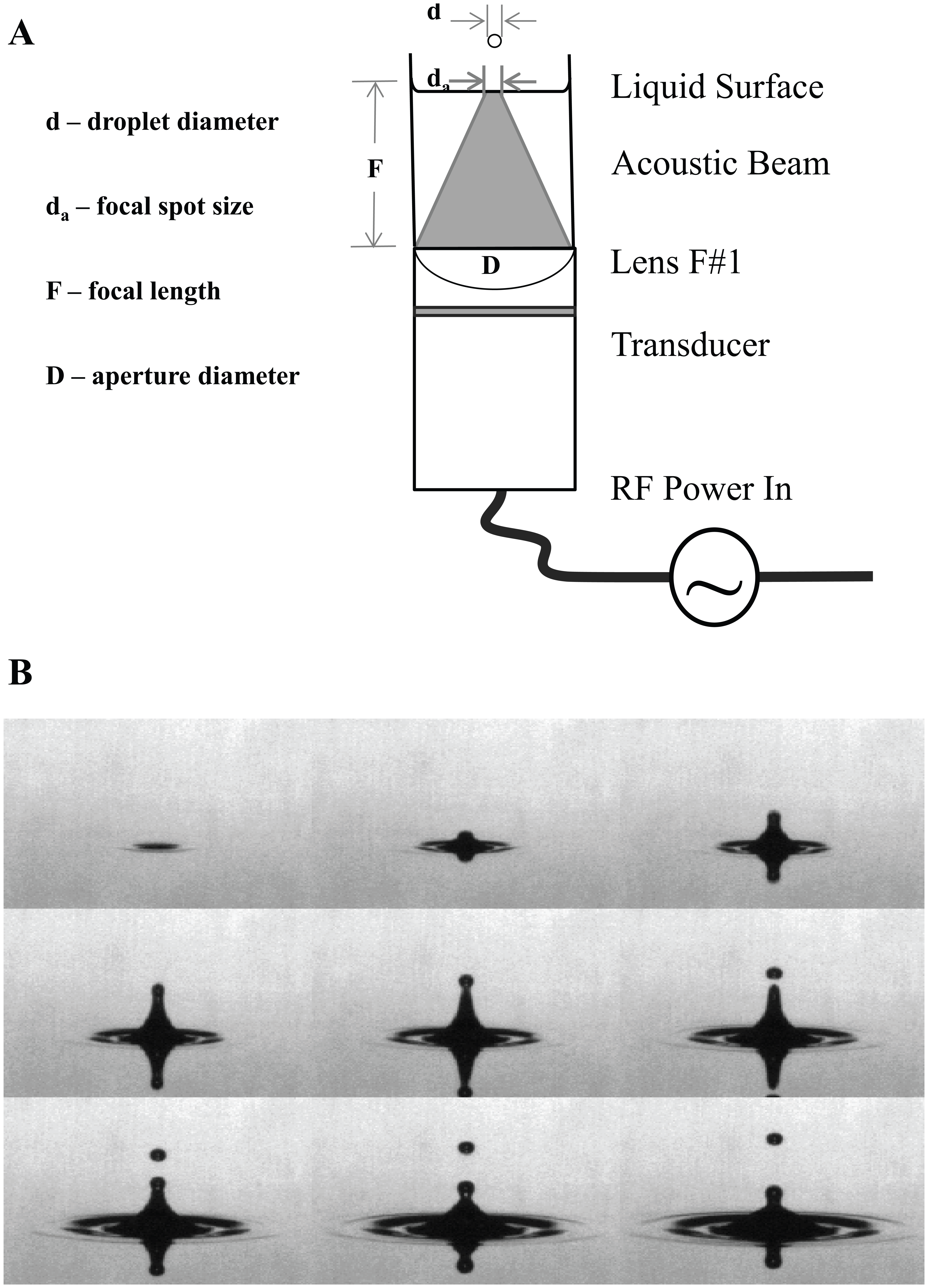
An early configuration of ADE focused acoustic energy at a liquid interface pinned to a nozzle, similar to ink-jet devices, with the size of the acoustic field comparable to the dimensions of the nozzle opening.⁹ Designs that concentrated acoustic energy at the surface of an “infinite pool” were also explored,¹⁰ and later, an intermediate “large pool” version was proposed by Quate and Khuri-Yakub¹¹ for printing applications, as it balanced constraining the fluid volume and interactions with the opening to avoid clogging. The ADE system of Figure 1A illustrates the basic configuration of Quate: a focusing transducer is immersed in a layer of fluid, and the free surface of the fluid is adjusted to be at the acoustic focus of the transducer. It is “nozzle-less,” as it consists of a focused acoustic transducer with an open liquid surface much larger than the dimensions d_a of the acoustic beam at its focal point near the liquid surface. The lens is designed to have a focal length of F and an aperture diameter of D. The ratio of F over D is known as the F-number (F#) of the lens, providing a measure of how sharply the acoustic beam is focused. Most of the initial work with single-fluid-layer ADE systems was performed with lenses having F# = F/D = 1, as shown in Figure 1A .

Figure 1.

(A) Basic configuration of an acoustic drop ejector involving direct contact of the focused acoustic energy source with the ejected liquid. (B) Time evolution of drop formation in an ADE system. The droplet shown here is 2.5 nL in volume and 168 μm in diameter. The time delay in illumination between each image is 50 μs.

The transducer is excited with a burst of radio frequency (RF) signal at a frequency of f. The transducer converts the electrical signal into ultrasonic waves and focuses the ultrasound toward the surface of the fluid layer. When the acoustic waves hit the fluid surface, they exert a momentum on the fluid surface due to the radiation pressure of the sound waves.¹² If the intensity of the acoustic field is sufficiently high, radiation pressure overcomes the restraining force of the surface tension and a mound is formed on the fluid surface. As the acoustic intensity is raised beyond a certain limit, typically described as the threshold of ejection, a droplet is ejected from the top of the mound due to the Rayleigh–Taylor instability.¹³ Figure 1B shows the time evolution of drop formation using ADE, generated by stroboscopically illuminating the fluid surface at various delay times after the application of the electrical signal into the transducer.

Elrod et al. have performed experimental and theoretical investigations of the basic acoustic drop ejector structure of Figure 1A .¹⁴ It has been shown that for a focused acoustic beam where F ∼ D, the ejected drop diameter, d, is fairly close to the width, d_a, of the ultrasonic beam at the focal point of the acoustic transducer. It should also be noted that the basic focusing structure in Figure 1A has been employed in scanning acoustic microscopy (SAM) applications, and the focusing characteristics of such structures have been studied extensively.^{15, 16} Based on these studies, the acoustic beam size, d_a, at the focus can be related to the ejector design parameters, as shown in eq 1.

d_{a} = 1.02 * F # * λ = 1.02 * F # * v / f

where F# = F/D is the F-number of the focusing transducer and λ and v are the wavelength and velocity of sound in the fluid layer, respectively. F and D are the focal length and aperture diameter of the transducer, respectively, and f is the acoustic drive frequency. Therefore, for a given fluid with a particular sound velocity, an ADE system can be designed to produce a desired drop diameter (hence a desired drop volume) by properly choosing the RF design frequency for a given acoustic focus geometry. We should also add that the ADE process produces drops with excellent reproducibility: the volume coefficient of variation (CV) is typically less than 2%.⁴

The dominant physics driving ADE has been shown to be remarkably unchanged over a wide range of frequencies covering more than two decades, producing droplet volume ranges spanning more than six orders of magnitude. With typical fluid sound velocities in the range of 1–2 km/s, typical RF drive frequencies range from about 1 to 200 MHz to generate drops in the subpicoliter to microliter range, with tonebursts in the microsecond to half-millisecond range.^11,14,17,22 With this flexibility in droplet volume, ADE has been employed in a variety of applications using a number of different fluids. Table 1 shows a summary of some applications utilizing ADE.

Table 1.

Various Applications Utilizing ADE That Show the Scaling of Drop Diameters and Drop Volumes with RF.

Droplet Diameter	Droplet Volume	Frequency	Application (with reference)
~10 µm	~1 pL	~150 MHz	Printing using aqueous and hot-melt inks¹⁷
~50 µm	~100 pL	~30 MHz	Spotting applications for cancer research¹⁸
~200 µm	1–10 nL	~10 MHz	HTS and other biological liquid handling applications^19,20
~1 mm	~1 µL	~1.50 MHz	Solder ball (microliter scale)²¹ Precision-selective Parylene coating for electronic applications²²

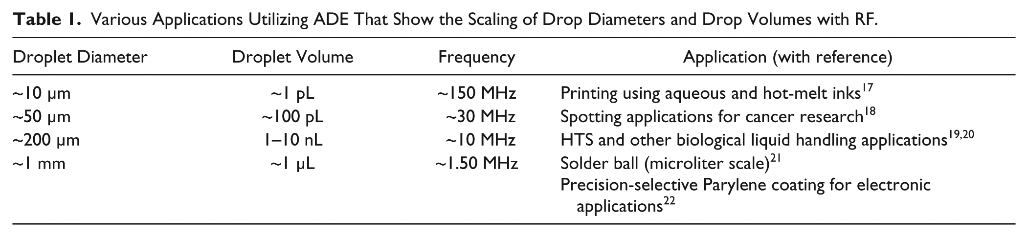
It should also be pointed out here that the observed dependence of the drop diameter on F# appears to be significantly less than linear for F-numbers around 2.¹⁴ If the drop diameter were to follow the acoustic spot size, we would expect the diameter to scale linearly with the F#, as suggested by eq 1. The reason for this discrepancy is not well understood.

Adapting ADE to HTS and Microplate Standards

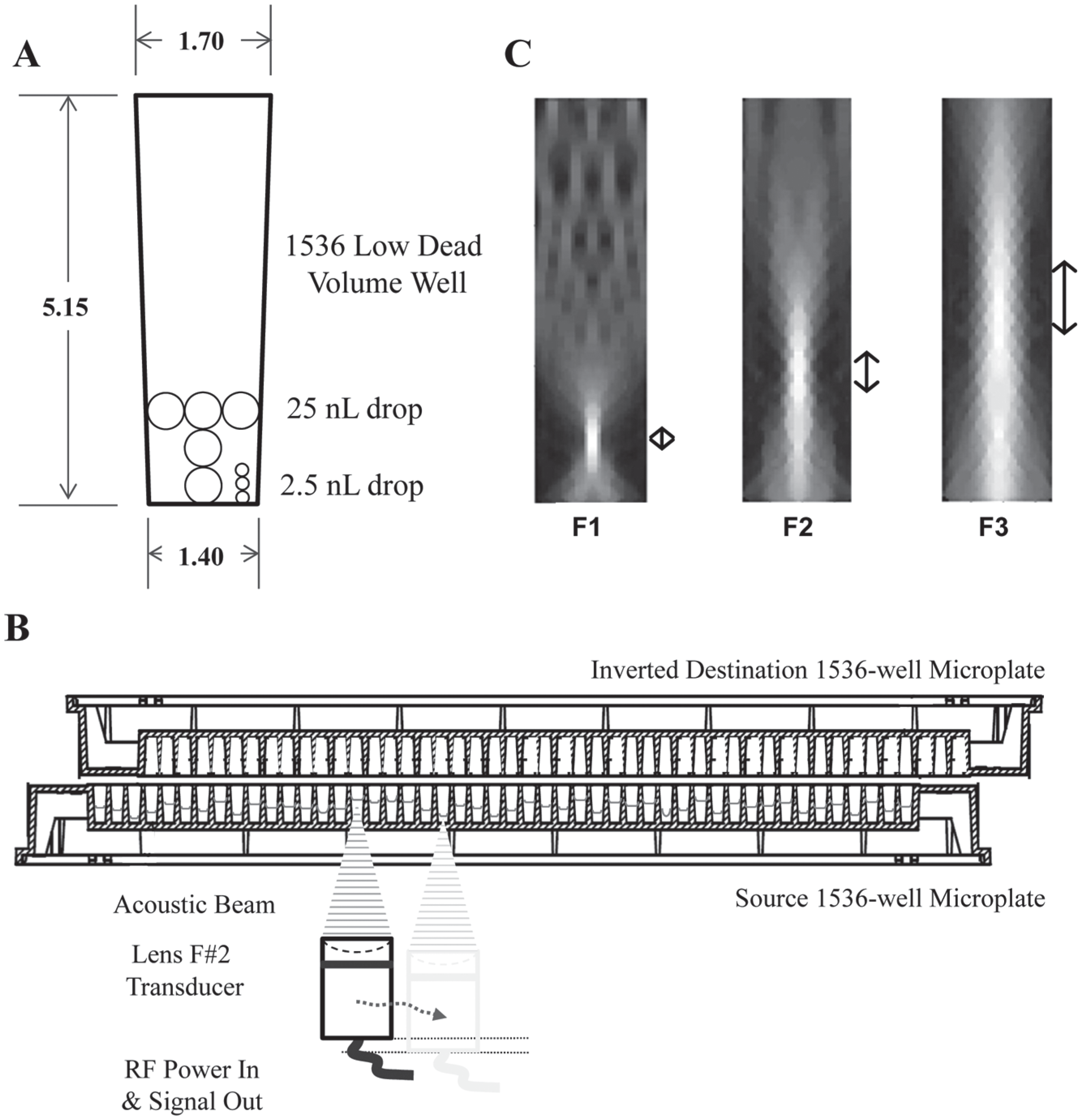
Many of the applications of Table 1 , however, are most useful when more than one material or analyte can be transferred. For the “open pool” methods of ADE, such as for black ink¹¹ or coatings,²² the acoustic generators were all exposed to the same common fluid. For multiple fluid applications, like high-throughput screening, acoustic energy must access many fluid reservoirs. Microtiter plates are commonly used to contain the variety of fluids for HTS applications. The “square” reservoir configurations of Figure 1A explored by earlier researchers differed from the geometry of wells of microplates, as microplate wells are generally taller than they are wide. Figure 2A illustrates a low-dead-volume (LDV) well designed for a 1536-well microplate with an aspect ratio of more than 3:1.

Figure 2.

(A) High-aspect-ratio microplate well where the height is 3.67 times larger than the well bottom width and roughly 3× the well top opening based on dimensions from the Labcyte 1536 Low-Dead-Volume Microplate (Labcyte, Sunnyvale, CA), shown in millimeters. Drop sizes for 2.5 and 25 nL, standard sizes for commercial ADE instruments, are shown to scale. Transfers of fluids down to liquid depths below three droplet diameters require precise power control to maintain precision and accuracy. (B) ADE configuration to eject fluids from microtiter plates based on the 1536 LDV well shape of A. Two transducer positions are indicated, for ejection from two different wells. For the position on the left, the transducer is moved upward to focus on the maximum fluid height before the acoustic beam is occluded. For the position on the right, the transducer is lowered to focus on the surface of a thinner fluid layer. The difference in volumes represents the acoustic well working volume. Note, in contrast to Figure 1A , the acoustic lens is F#2 to enable a larger working volume. (C) Model of acoustic focusing in a water-filled well of a 1536 LDV microplate with lens designs of varying F#: 1, 2, and 3. A 10 MHz acoustic beam enters the well from the bottom and propagates upward. The beam is positioned relative to the bottom so that only 10% of the acoustic energy does not enter the well fluid due to occlusion. Lighter color indicates higher acoustic pressure from the beam. The arrows to the right of the images indicate the usable “depth of focus,” the range of fluid depths for which the acoustic intensity is within approximately ±2% of the peak intensity, and correspond to the 1:4:9 ratio for the square of the F# in eq 2.

Most biological applications such as HTS require a large number of different fluid samples as well as their delivery in rapid succession from a source microplate to a destination microplate. Application of ADE to microplates for HTS automation requires a change in typical transfer configurations in order to align the droplet trajectory of the source microplate well with the destination. Hence, the inclusion of mechanisms to invert destination plates to integrate with standard microplate automation robotics is also needed. The use of “sonar” to locate the liquid–air interface has also been described.⁴ For the configuration of Figure 1A with the acoustic source and lens in direct contact with the fluid, the liquid surface reflection is unambiguous. For indirect configurations, as is required for an acoustic transducer located external to the fluid container, as in the case of a source microplate well in Figure 2B , the sonar results contain multiple reflections, as acoustic waves emitted from the transducer first go through a “coupling fluid,” which is typically water, and then through the bottom of the microplate before entering the well fluid. Note that in Figure 2B , the acoustic path length through the coupling fluid changes, as the transducer height is adjusted to compensate for the change in fluid height from well to well.

As the acoustic waves impinge on the plate bottom, they are partially reflected and partially transmitted into the source fluid, where the waves continue to focus toward the well fluid surface for droplet ejection. The most commonly used well plates are made of plastic materials such as polypropylene or cyclic olefin copolymer (COC). Fortunately, these plastics are generally acoustically “transparent,” such that the acoustic waves go through without a significant loss at the typical low-megahertz frequencies employed in most biological applications. Nevertheless, as will be described in subsequent sections, such a double-layer configuration poses significant challenges in the system design and operation, in order to meet the demanding requirements of typical biological fluid-handling applications.

Desirable ADE Attributes for Biological Fluid Handling

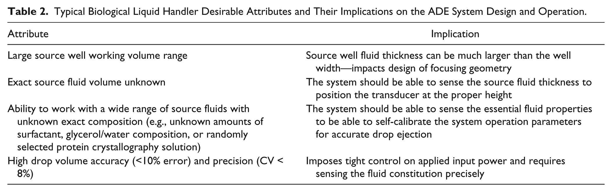
In most biological liquid-handling applications, it is desirable to be able to transfer fluid volumes as fast as possible, with very high accuracy and precision, and with minimum user intervention. Table 2 summarizes some typical system usage requirements and their implications from the point of view of the design and operation of an ADE system. These implications are clarified further in subsequent sections of this article.

Table 2.

Typical Biological Liquid Handler Desirable Attributes and Their Implications on the ADE System Design and Operation.

Attribute	Implication
Large source well working volume range	Source well fluid thickness can be much larger than the well width—impacts design of focusing geometry
Exact source fluid volume unknown	The system should be able to sense the source fluid thickness to position the transducer at the proper height
Ability to work with a wide range of source fluids with unknown exact composition (e.g., unknown amounts of surfactant, glycerol/water composition, or randomly selected protein crystallography solution)	The system should be able to sense the essential fluid properties to be able to self-calibrate the system operation parameters for accurate drop ejection
High drop volume accuracy (<10% error) and precision (CV < 8%)	Imposes tight control on applied input power and requires sensing the fluid constitution precisely

Focusing Transducer Design for Biological Fluid Handling Applications

Experimental and theoretical work for nonbiological applications of ADE largely addressed focusing elements with an F# of 1, where the focal length of the lens was equal to the lens aperture diameter. From a simple, geometrical focus perspective, F# = 1 would limit the maximum depth of the source well fluid that can be accessed to a level that is approximately equal to the well bottom width. For thicker fluid layers, one would expect higher acoustic loss due to the occlusion of the acoustic beam by the well bottom opening. However, as described in Table 2 , for most biological applications, it is desirable to address a large range of source well fluid volumes with the ADE instrument to make better use of the volume in commercial microplates due to their higher aspect ratios (well height to well bottom). Therefore, it is preferred to optimize the lens design to meet the design requirements of achieving focus in the well that is higher than a distance roughly the width of the well bottom to avoid occlusion loss and compensate for the higher attenuation losses due to the longer path of travel for the acoustic beam from the transducer to the liquid surface.

In order to understand the dependence of the maximum ADE addressable fluid depth on the lens F# and optimize the lens design parameters, we have analyzed the acoustic focusing behavior using a wave diffraction model.¹⁶ Figure 2C shows the results of this analysis for lens designs with F-numbers of 1, 2, and 3, using the well geometry of Figure 2A with a bottom opening of 1.4 mm, sound frequency of 10 MHz, and well fluid that has the same sound velocity as water. The figure shows the maximum fluid depths that can be used with each lens design, in order to limit the power loss due to beam occlusion to approximately 10%. It is fairly clear that an F# of 1 limits the usable source fluid volume significantly compared to the other designs.

From the images of the three beams in Figure 2C , it is also evident that the depth of focus of the acoustic beam increases with the F-number. That is, as the F-number is increased, the range of fluid depths near the focal point of the lens where the acoustic intensity is nearly constant increases. This variation of depth of focus with lens F-number is a fundamental property of the beam focusing. For example, for a simple focused beam in a single fluid layer, the depth of focus t_DOF is shown to be as given in eq 2 for a criterion of a 50% drop in acoustic intensity.¹⁶

t_{D O F} = 7.1 * {(F #)}^{2} * λ = 7.1 * {(F #)}^{2} * v / f

This equation shows that the depth of focus increases as the square of F#, which should result in a more relaxed tolerance for focus positioning, as the F# is increased. However, as will be discussed later in the section on acoustic power control requirements, it would be too optimistic to use a 50% criterion in order to come up with a specification on the allowable focus distance error to achieve a tight droplet CV. Based on the acoustic field calculations of Figure 2C , we estimate that the maximum error in transducer focus positioning should be approximately ±100 µm in order to cause a negligible error in the acoustic intensity at focus for ADE to generate 2.5 nL drops with the F#2 lens. The allowable error in transducer focus position for an F#1 lens would be considerably smaller, of the order of ±25 µm.

As discussed in Table 2 , for most biological applications, the well fluid height is not known, and the instrument must “audit” the well fluid contents to estimate the fluid thickness, just prior to drop ejection. Any error in this estimation will result in an error of the positioning of the acoustic transducer height to place the fluid surface near the focal point of the transducer. A larger F# allows more tolerance for both fluid thickness estimation and transducer height adjustment. Thus, selecting F# > 1 gives more efficient drop ejection from fluids whose depth is greater than the well width and results in a lower sensitivity to focus errors due to the transducer position relative to the fluid surface.

Auditing

To eject drops from multiple wells of a microtiter plate, with each well possibly containing a different fluid and filled to a different height, it is necessary to sense the fluid in each well, prior to ejecting drops. This sensing, or auditing, of the well fluids must be done rapidly to achieve high throughput. It is convenient that the same acoustic configuration used to eject the drops (e.g., see Figure 2B ) can be used to audit the fluid in each well. In order to audit the well fluid, the focused transducer is situated beneath the well, and a short (~1 cycle) “ping” excitation is applied to the transducer to create an acoustic pulse that propagates from the transducer to the free surface of the well fluid, and back. A portion of the acoustic energy is reflected each time the pulse encounters an interface. These reflections are then recorded at the transducer, so that in this auditing mode, the transducer both transmits the short auditing ping signal and receives the echoes from the well plate and fluid.

The recorded reflections yield information regarding the well fluid depth, as well as information regarding an important acoustic property of the well fluid: its acoustic impedance. The acoustic impedance, Z, of a fluid is defined as the product of the fluid density ρ and the speed of sound v in the fluid: $Z = ρ * v$ . A typical unit for acoustic impedance is the MRayl, which corresponds to 10⁶ kg/m²-s. To understand the auditing signal, it is convenient to first consider what happens to the acoustic beam as it encounters a single interface (e.g., that between the well bottom and well fluid). In doing so, it is simplest to treat the acoustic beam and its reflections as simple plane waves, and to assume the acoustic beam interacts with an ideal interface at normal incidence. In this case, the reflection and transmission of the acoustic beam are simple to interpret.

At a simple interface, a planar compressional acoustic beam normally incident on that interface will be partially reflected. The amplitude reflection coefficient is readily expressed in terms of the acoustic impedances of the two materials that form the interface. If the acoustic wave is traveling from material 1 into material 2, as indicated in Figure 3A , the amplitude A_r of the reflected wave is given by the simple expression

A_{r} = A_{i} * (Z_{2} - Z_{1}) / (Z_{2} + Z_{1})

Figure 3.

(A) Reflection and transmission of an acoustic plane wave normally incident on an ideal interface. (B) Plots of the amplitude reflection and power transmission through a plastic–fluid interface.

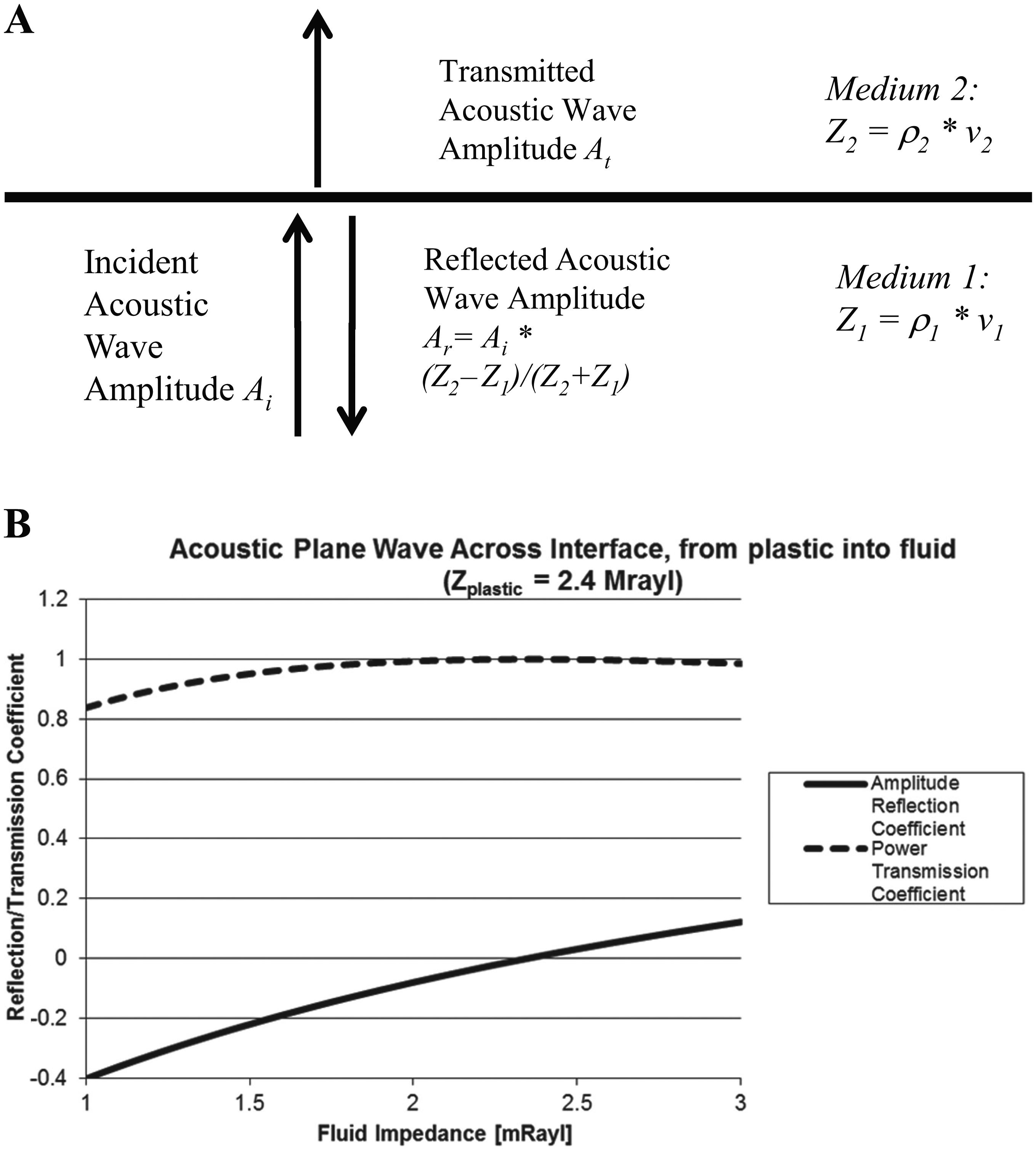
Here A_i corresponds to the amplitude of the incident wave, and Z₁ and Z₂ correspond to the acoustic impedances in materials 1 and 2, respectively. Figure 3B shows a plot of the ratio A_r/A_i for an acoustic compressional wave traveling from plastic (Z = 2.4 MRayl) into a fluid of varying acoustic impedance. Also shown in the plot is the acoustic power transmission coefficient across the interface. It is evident from the form of eq 3 and the plot of Figure 3B that the magnitude of the acoustic reflection at the interface between two media increases as the difference between the acoustic impedances of the two media increases. It is also evident that if the acoustic properties of one of the media are known, then from the acoustic reflection at the interface, the acoustic impedance of the second medium may be calculated.

Acoustic Signal Processing of Sound from Microplate Wells

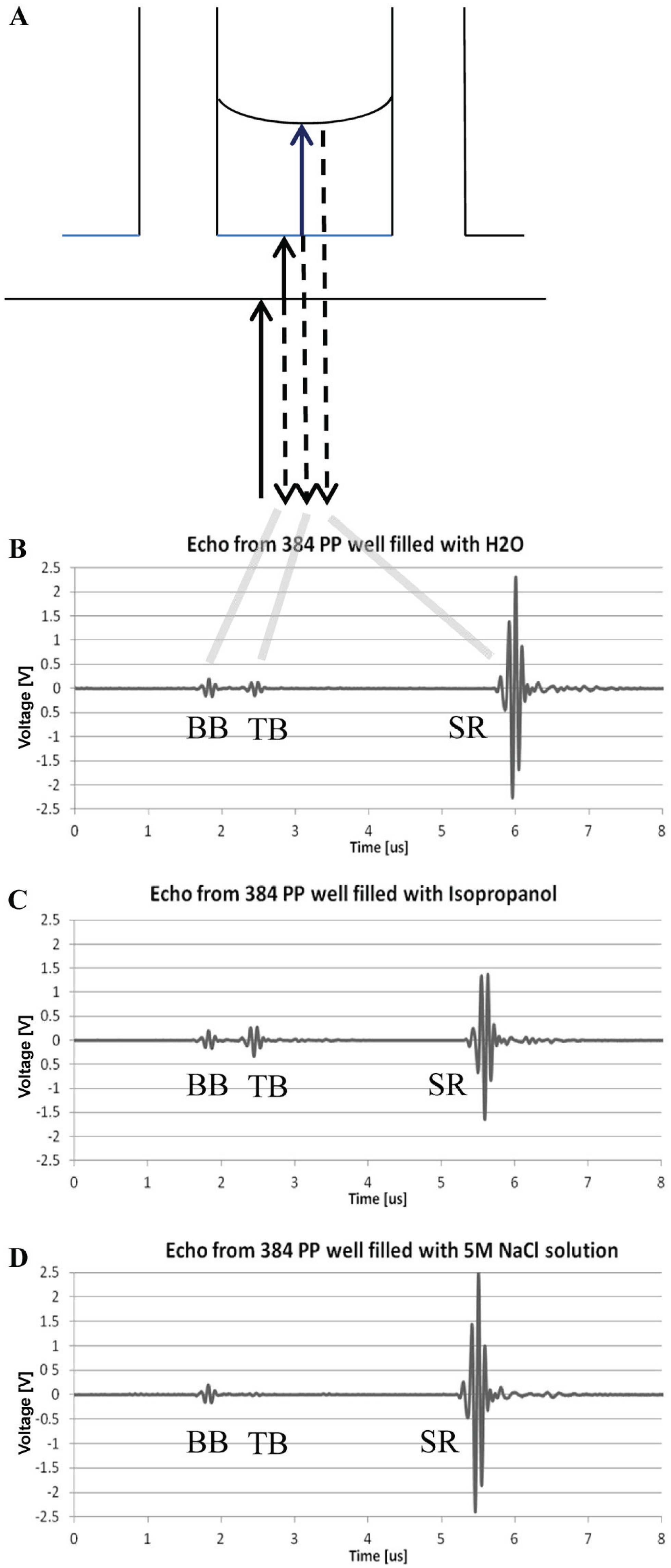
In auditing, the acoustic auditing pulse travels from the transducer, through the well bottom, and into the well fluid. The signal is then reflected nearly completely from the well fluid–air interface (the acoustic impedance of air is much less than any fluid) back to the transducer. For the configuration of a multiwell plate, there are three major echo components, which are usually labeled bottom of well bottom (BB), top of well bottom (TB), and surface reflection (SR). The origins of the three components are indicated in Figure 4A . The BB echo is associated with the reflection from the coupling fluid–well bottom interface. The TB echo is associated with the acoustic reflection at the well bottom–well fluid interface. The SR echo corresponds to the reflection at the well fluid–air interface. From eq 3, the TB echo amplitude will be sensitive to the acoustic impedance of the well fluid, and is thus of particular interest in sensing the well fluid acoustic properties.

Figure 4.

The origin of the acoustic audit signal for a filled well. (A) There are three main echo components: BB, TB, and SR. These are due to reflections at the coupling fluid–well bottom interface, the well bottom–well fluid interface, and free surface of the well fluid, respectively. Audit echo signals from a 384-well polypropylene plate sequentially filled vary with impedance for different fluids: (B) water (Z = 1.49 MRayl), (C) isopropanol (Z = 0.93 MRayl), and (D) 5 M NaCl solution (Z = 2.11 MRayl).

Figure 4B–D show audit echo signals from the same well filled with three fluids of varying acoustic impedance. For the low-impedance fluid isoproponal (Z = 0.93 MRayl) in Figure 4C , the TB/BB ratio is quite large compared to that of water in Figure 4B . For the 5 M NaCl solution in Figure 4D , whose acoustic impedance is large (Z = 2.11 MRayl), and hence closer to the impedance of the well bottom (Z = 2.4 MRayl), the TB/BB amplitude ratio is quite small. Indeed, it may be noted in the figure that the BB echo amplitudes are all nearly identical, as would be expected, since the coupling fluid–well bottom interface is the same in all cases. The BB echo amplitude serves largely as a normalization factor, to account for differences in the driving electronics or transducer efficiency.

From the above plots of Figure 4 , one clearly sees the effect of the well fluid impedance on the relative amplitudes of the TB echo components. This effect may be used in a quantitative manner to determine the acoustic impedance of a given well fluid. The sensitivity of the measurement is evident in the data of Figure 5 . Here, for sodium chloride solutions in water, a plot of the measured TB/BB amplitude ratio versus the known acoustic impedance is shown (plate used is a 384-well polypropylene microtiter plate). The NaCl solutions vary from 0 M (Z = 1.49 MRayl) to 5 M (Z = 2.11 MRayl). From the measured data shown in Figure 5 , it is quite clear that for a NaCl solution of unknown molarity, one could readily use the TB/BB ratio to determine the NaCl concentration.

Figure 5.

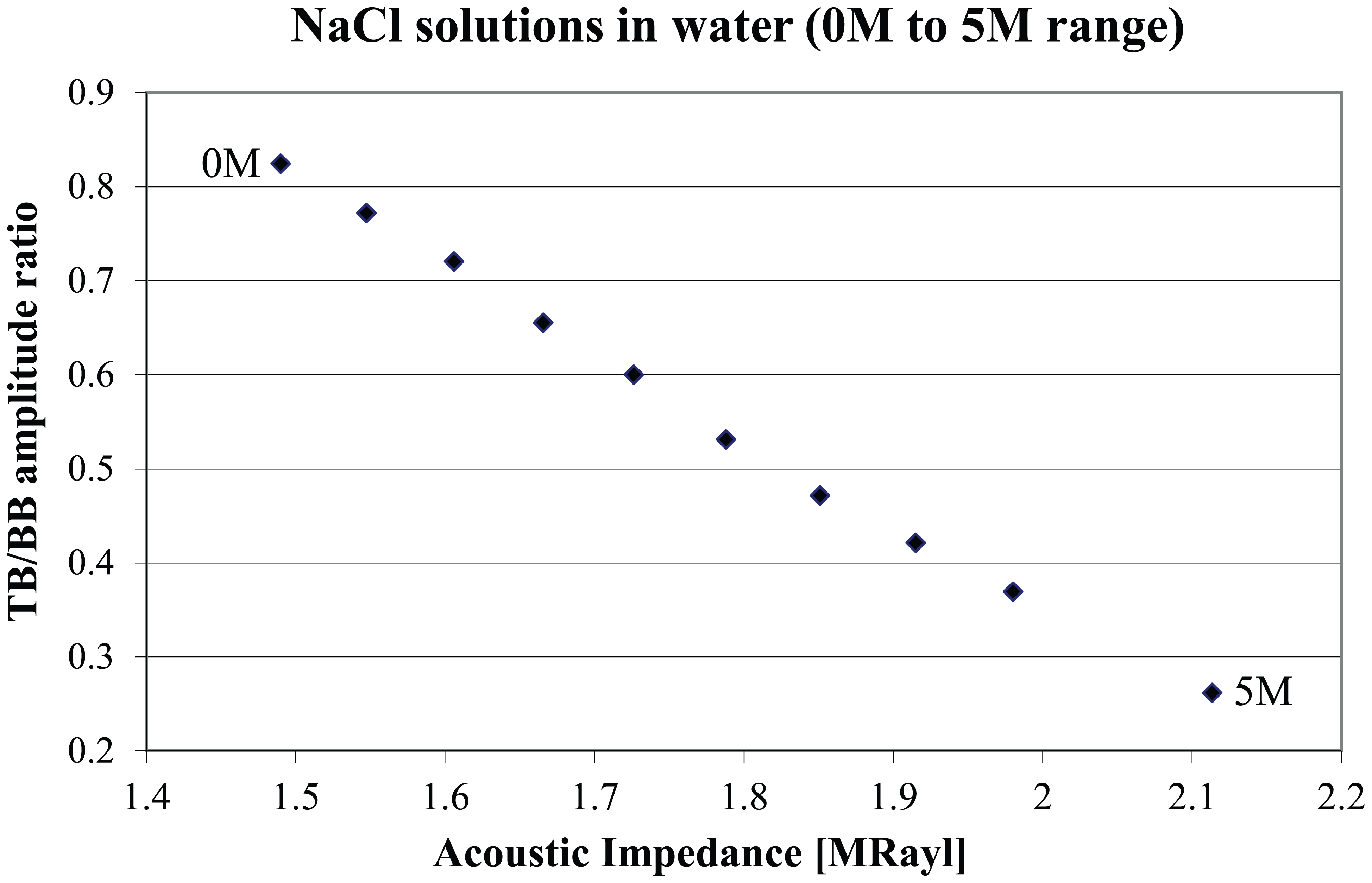
Measured ratio of TB/BB echo amplitudes for NaCl solutions of varying molarity.

Thus, from acoustic auditing, one may extract the acoustic impedance of the well fluid.^{23, 24} If one is working within a characterized set of fluids, for example, glycerol/water or salt solutions, one can use the acoustic impedance measurement to determine the concentration (i.e., glycerol or salt concentration), and hence infer the full set of physical properties of the well fluid. If the well fluid composition is entirely unknown, it is still possible to use the acoustic impedance measurement to estimate the speed of sound in the well fluid, for example, by assuming a given fluid mass density. Having estimated the acoustic velocity in the well fluid, and knowing the time separation between the TB and SR echoes, the well fluid depth is then calculated (the time separation multiplied by the speed of sound in the well fluid is simply twice the well fluid thickness). Using a simple model of the focusing of the transducer into the well plate, it is then possible to calculate exactly what height to place the transducer beneath the well, in order to focus the acoustic beam at the well fluid surface.

It will be recalled that the above analysis of the echo information assumes acoustic compressional plane waves. For focused acoustic waves, the relations are somewhat more complicated, as the ratio of the TB/BB amplitudes is also a function of the distance of the well bottom from the transducer. To account for this, all auditing is performed at a constant distance between the well bottom and the transducer (the BB echo signal occurs at a constant time), and the effects of the focused beam on the TB/BB amplitude ratio are taken into account.

The above discussion also assumes normal incidence of the acoustic plane waves, and neglects conversion of longitudinal waves into shear waves within the well bottom plastic. This effect is small, but measurable—it is generally acceptable to ignore the shear wave effects. Finally, we have not discussed in the above description any effects due to attenuation of acoustic waves. In general, acoustic waves will attenuate in both fluids and plastics. Thus, for example, there is some decrease in the acoustic amplitude as the auditing pulse travels through the well plate bottom, which should be taken into account in the ratio of the TB/BB echo amplitudes. For microplate materials such as COC, this loss is relatively small, but again measurable. These attenuation effects can be taken into account as needed.

Simple acoustic auditing therefore may be used to extract information regarding the acoustic impedance and thickness of the well fluid. This measurement is very fast—each echo waveform in a well is captured within tens of microseconds. Since the audit measurement is performed with a fixed height of the transducer relative to the well plate, it is possible to scan over the well plate rapidly and audit all relevant wells efficiently, before ejecting drops. At the end of auditing, the fluid thickness in each well is calculated, and the appropriate transducer height relative to the well bottom is determined for drop ejection. It is still necessary to determine the appropriate acoustic power required for stable drop ejection, and the methods to do so will be described in the following sections of this article.

RF Power Control Requirements

Drop ejection using focused acoustics exhibits a threshold phenomenon; when the input power is below a critical value, there will be no drop ejection. As the power is raised above this value, one observes increasingly higher velocity drops.²⁰ From the point of view of the robustness of drop transfers, it is desirable to achieve a certain minimum drop velocity to avoid drops not reaching the destination, due to viscous drag or gravitational forces. The ejected drops would need to travel a distance of about 25 mm, for example, between two 384-well source and destination plates. A drop velocity of about 1 m/s has been determined to be a good minimum target velocity based on experimental studies. As the input power is increased further, one generally observes the generation of secondary “satellite” drops. Satellite drops have the tendency to degrade the precision of drop ejection and may also lead to contamination concerns, so avoiding the satellite threshold is critical. The constraints described on the power above require the acoustic power received at the focal spot to be within the intensities required for sufficient upward drop velocity, while staying under the satellite threshold to ensure robust, precise fluid transfers.

In addition to the requirements on the absolute input power range described above, it is generally observed that the ejected drop volume shows a variation with input acoustic power, which may restrict the range of acceptable power levels even further, in order to meet the desired, tight drop volume accuracy and precision requirements for HTS (see Table 2 ). Modeling of the dependence of ejected drop volume as a function of input power is extremely complex, so one has to resort to experimental measurements. The behavior of drop volume variation with power was explored previously for low F-numbers close to 1.¹⁴

For F#1 focusing, the drop volume was found to be quite sensitive to the acoustic power received at the focal spot near the fluid surface, making it difficult to achieve in practice the desired drop transfer precision when the well plate and well fluid properties (including fluid height) are not precisely known to a tight tolerance. Fortunately, as seen in Figure 6 , the measured variation of drop volume as a function of input power for a lens with an F# of 2 exhibits the favorable characteristics of having both a longer depth of field for the focus and a reduction in droplet volume with increasing power after achieving the ejection threshold. In Figure 6 , there is seen a shallow “bowl” region in the drop volume, as the acoustic power is increased above the drop ejection threshold value. In this bowl region, the drop volume is seen to remain relatively flat, which affords a usable and practical operating range of ejection power.²⁵ In addition, the CV of drop volume variation in the bowl region is also generally low, as indicated by the error bars in the plot. Based on the plot of Figure 6 , we can assert that the RF signal amplitude has to be controlled to within about ±4%, in order to achieve the target drop volume CV specifications.

Figure 6.

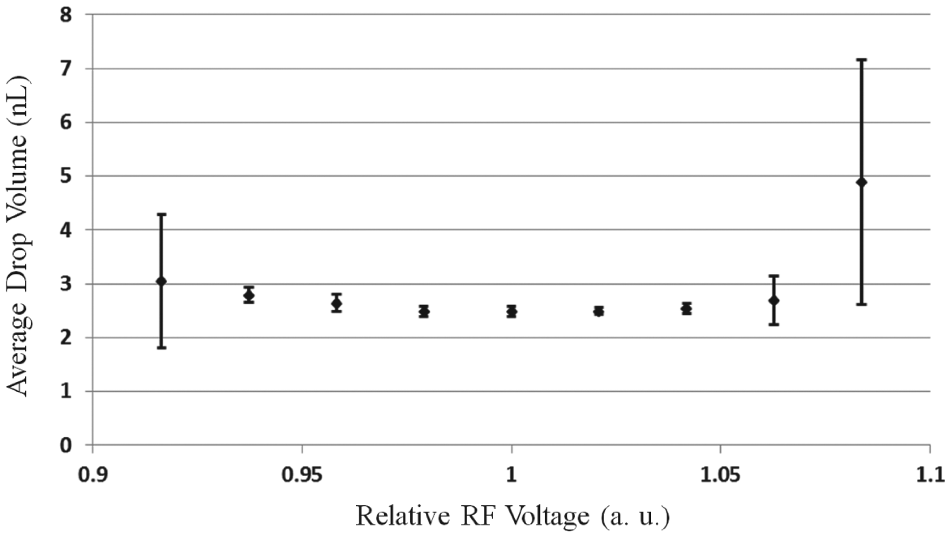
Drop volume vs. RF input signal amplitude (in arbitrary units) for focusing at F# of 2, for a target drop volume of 2.5 nL. The error bars show the standard deviation of the measured drop volume at each voltage setting.

The relatively tight target input-power accuracy value obtained above poses a significant challenge regarding the calibration of the instrument, as there may be somewhat significant uncertainties in the system gain from the transducer to the focal point. There is acoustic attenuation in all of the propagation media, and while the attenuation is low in the coupling fluid (water) and common microplate plastics near 10 MHz, attenuation can be appreciable in some well fluids. Also, there are reflections at the fluid–well bottom interfaces that will affect the amount of energy that is transmitted to the well fluid surface. These attenuations and reflections, along with the rheological properties of the well fluid itself (viscosity, surface tension, etc.), determine the acoustic power needed at the transducer to eject a drop from the well fluid surface. For well fluids of a known class (e.g., glycerol/water), the information from auditing alone (well fluid Z and fluid height) may be used to predict the fluid properties in the well, and thus allow for robust drop ejection. If the well fluid class is unknown, the auditing information will only partially suffice to determine the optimum drop ejection parameters. In particular, for an unknown fluid, after simple auditing, it may not be possible to predict the precise RF power required for optimal drop ejection. For this case, as well as to relax the general system constraints imposed by the ±4% acoustic amplitude window for ejection, a second real-time acoustic measurement has been developed. In this second measurement, as will be described in detail in the following section, the well fluid surface is first perturbed using an initial acoustic excitation, and then this perturbation of the surface is sensed, using a second acoustic auditing pulse. This dynamic measurement of the well fluid allows one to calibrate in real time to the well fluid properties, in order to adjust the RF power for acceptable drop ejection.

Dynamic Fluid Analysis

Dynamic fluid analysis (DFA) makes use of an interferometric perturbation measurement to characterize the dynamic response of the fluid surface to the acoustic energy in real time, without ejecting drops. From such a measurement, one may determine the optimal acoustic power for actual drop ejection. The measurement is based on the creation of a subejection mound at the fluid surface, using generally the same acoustic RF signal, or toneburst, that is used for drop ejection, but whose energy is 2–3 dB below that required to eject a drop. In performing DFA, the acoustic transducer is first moved beneath a well, to a height such that the acoustic beam is focused at the well fluid surface (this assumes that the normal auditing has already been performed, to determine the proper transducer height for ejection). A lower-power acoustic ejection toneburst is excited, producing a mound at the fluid surface, which rises and falls without ejecting a droplet. At a fixed time delay following the excitation of the subejection acoustic toneburst—when the mound is well formed—a short audit ping is excited, and the echo of this ping from the perturbed well fluid surface is measured. The interaction of the echo pulse with the fluid mound occurs over microseconds; the mound is essentially static over this timescale, so that the echo pulse can be thought of as interacting with the mound in a static position, at a given moment in its development.

The presence of the mound is found to “split” the echo from the well fluid surface into several distinct subcomponents. Measurement of these components in turn provides information regarding the mound size. Some simple simulations of acoustic propagation help to visualize what is happening. In Figure 7A–D are shown a set of echo simulation results. Along the left-hand side of Figure 7A–D are shown layout cross sections for the sequence of simulations. The transducer is at the bottom of each layout figure, and the well fluid meniscus is at the top. Progressing from the top layout image to the bottom, the mound size is increased at the fluid meniscus. The physical dimensions of each cross section figure are 3.8 mm wide × 7.6 mm tall. In the simulations (full three-dimensional [3D]), the wells looked at from above are square (3.8 mm × 3.8 mm), and the spherical acoustic transducer has an F-number of 2.

Figure 7.

The cross sections of wells (left) and their echo waveforms (right) are shown for 3D acoustic propagation simulations involving four different mound heights at the well fluid surface. The F#2 transducer is at the bottom of each well cross section, and the fluid meniscus at the top. From A to D, the simulated perturbation mound height at the center of the free fluid surface progressively increases. The waveform shown at the right of each well (A–D) is the calculated echo reflected from a sound pulse interacting with the upper and lower surfaces of the well plate bottom (at 2 and 3 μs, respectively) and then the SR component (near 7 μs) showing an increased splitting of the SR waveform as the mound size increases.

To the right of each layout cross section in Figure 7A–D are shown the associated echo waveforms that are calculated in the simulations, assuming a short ping excitation of the transducer. As the mound height increases, one sees that the simulated SR echo signal actually splits into three components. The location of the first component is aligned with the location of the echo from the unperturbed fluid surface. The locations of the second and third components are associated with the shape of the mound itself. From other simulations in which the mound shape is varied, it has been determined that the third component (that furthest out in time) is generally due to reflection from the top of the mound. The middle component is due to a multiple reflection from the angled base of the mound. The first component is due to reflection from the annular region of the largely unperturbed fluid, outside of the mound.

From the simulations, as well as from experiment, it is thus found that the splitting of the SR echo signal is a measure of the mound size. Thus, in a DFA measurement, the splitting of the SR echo is extracted, and this yields information regarding the size of the subejection mound that has been formed, following the excitation of the transducer with a known subejection toneburst signal. From this information, it is generally possible to predict the acoustic energy required to actually eject the drop, as will be shown.

To measure the splitting of the perturbed SR echo in practice, some signal processing is required. Typically, to simplify the measurement, the first component of the split echo signal is removed, and only the second and third components are analyzed. Next, it is convenient to apply a fast Fourier transform (FFT) to the echo signal and work in frequency space. Figure 8 shows a typical DFA result for a 30% glycerol solution in water. The split SR echo resulting from the perturbed surface is shown in Figure 8A with the second and third echo components selected. Figure 8B shows the FFT of this signal. The splitting of the echo signal in time produces a set of minima in frequency space: two distinct minima at 7 and 8.9 MHz, respectively. The distance between the minima in frequency space is inversely related to the separation in time of the SR echo components. It is this spacing in frequency between minima that is then measured, as characteristic of the mound size. In the plot of Figure 8B , the minima spacing corresponding to the DFA measurement would be 1.9 MHz.

Figure 8.

Data from a DFA measurement of 30% glycerol in water, in a 384-well polypropylene plate. (A) Perturbed DFA echo with the first component of the echo removed. (B) FFT with two minima clearly present at 7 and 8.9 MHz. (C) Plot of the logarithm of the minima spacing in megahertz, M_S, as a function of the relative subejection toneburst energy (in decibels), for a DFA measurement on 30% glycerol in water.

A sequence of DFA measurements can be made using different subejection acoustic toneburst energies. This essentially reproduces experimentally the set of data that was simulated earlier, in Figure 7 . If one begins at very low subejection toneburst energy and sequentially increases the toneburst energy, one obtains a series of minima spacings. One may plot the minima spacings in megahertz as a function of subejection toneburst energy. It is convenient to plot the relative toneburst energy in decibels and the logarithm of the minima spacing in megahertz. In Figure 8C , a plot of the logarithm of the minima spacing, M_s, in megahertz is shown, as a function of subejection toneburst energy in decibels, for the same well filled with 30% glycerol, whose DFA measurement was shown in Figure 8A , B .

As can be seen, the dependence of the logarithm of the minima spacing in megahertz on the subejection toneburst energy in decibels is quite linear. This is very useful—it implies that from a measurement of the perturbation to the fluid following a single subejection toneburst, one may predict the perturbation that will result from tonebursts of other energies, if a good estimate of the slope of the curve in Figure 8C is known. If the fluid is entirely unknown, then a small number of measurements at different subejection toneburst energies will suffice to determine the slope of the line in Figure 8C .

In order to use this measurement to predict the acoustic energy needed for drop ejection, it is necessary to relate a given mound height—or in terms of the DFA measurement, a given minima spacing in megahertz—to a minima spacing that corresponds to the ejection of a drop. For a given class of fluids in which one is interested, this may be done directly by measuring independently the acoustic toneburst energy that corresponds to the threshold of drop ejection. Call this drop ejection threshold toneburst energy E_threshold and the subejection toneburst energy used in any given DFA measurement E_DFA. Noting from Figure 8C that the logarithm of the minima spacing in megahertz, M_S, varies linearly with the logarithm of the subejection toneburst energy (i.e., varies linearly with the subejection energy when expressed in decibels), we may write the general relation

10 * \log 10 (E_{DFA} / E_{threshold}) = A * \log 10 (M_{S}) + B

The coefficients A and B then define the relation between the minima spacing measured in a DFA measurement and the drop ejection threshold. These coefficients are characteristic of a given fluid, and once measured for a fluid, they can be used to immediately predict how much additional acoustic power is required to eject a drop, from a single DFA measurement on that fluid. Thus, for a characterized fluid in which the A and B coefficients have been measured, use of DFA can allow some relaxation of the tight tolerances that it would otherwise be necessary to maintain across an entire acoustic ejection system. Variations in transducer efficiency, or attenuation losses and reflections through the acoustic propagation path, can be readily compensated for, using the DFA measurement in real time.

Of significant importance, it is found that DFA may also be extended to uncharacterized fluids. To understand how this may be the case, it is useful to consider some measured values of the A and B coefficients in eq 4.

Table 3 shows some measured values for the coefficients A and B, over a number of fluids, for an acoustic toneburst center frequency of 11 MHz. It may be noted that the fluids encompass a reasonably large range of surface tensions and viscosities. Note that the coefficient B is nearly constant across these fluids. Looking at eq 4, it is evident that the value of B corresponds to just how much additional acoustic energy is required to just eject a drop (in decibels) when the DFA measurement produces a minima spacing of 1.0 MHz.

Table 3.

Some Typical Values of the A and B Coefficients Used in DFA Analysis for Various Fluids (2.5 nL Ejection at 11 MHz).

	Water	Isopropanol	100% DMSO	70% DMSO	Silicone Oil (Dow 200)	Ethylene Glycol
A	−0.78	−1.01	−1.25	−1.35	−0.74	−1.62
B	−0.58	−0.57	−0.57	−0.66	−0.49	−0.56

The fact that the B coefficient is relatively constant across many fluids is a rather surprising result. While the fundamental physics of this is not well understood, this empirical result does enable the DFA measurement to be extended to many fluids that are not well characterized. For previously untested or uncalibrated fluids, it is possible, for example, to perform the DFA measurement at several subejection toneburst powers, in order to determine the coefficient A (i.e., the slope of the relation between acoustic toneburst energy and the logarithm of the minima spacing in megahertz). Having determined A, one can simply assume a value of B, for example, B = −0.57. One can then apply eq 4 to determine the ejection threshold toneburst energy. Over a significant range of fluids, this assumption of a constant value for B results in a final toneburst ejection energy that is well within the power window for successful transfer of drops.

The DFA measurement is thus seen to be quite useful in allowing one to determine the correct ejection power, for both characterized (A and B coefficients known) and uncharacterized (A and B coefficients unknown) fluids. It is critical that the measurement always maintains an acoustic toneburst energy that is well below the ejection threshold. For fluids that are completely uncharacterized, this may mean that one must perform the DFA measurement beginning with a very low-energy toneburst, and repeat the measurement multiple times, sweeping the toneburst energy higher, until a sufficiently large mound is formed to produce a reasonable minima spacing. This method is illustrated in Figure 9A .

Figure 9.

(A) Dynamic fluid analysis method uses an interferometric interrogation process to find acoustic droplet ejection power as implemented in Echo liquid handling instruments (Labcyte). Starting at an energy known to be below the drop ejection power for the selected liquid class, the instrument performs a fast measurement to see if the power is close to the ejection level. If not, the power is raised and another attempt is made until the ejection power is determined. (B) Measured transfer volume from wells filled with 200% CMC SDS, in 1× PBS buffer. The intended transfer volume is 50 nL, from each source well of a 384-well plate. In the plot, each data point represents a 20-drop transfer of 2.5 nL droplets from 384 separate source wells.

Fortunately, the DFA measurement may be performed quite rapidly; the rise and fall times of the mound associated with a 2.5 nL drop are of the order of hundreds of microseconds.¹⁴ If the DFA measurement must be iterated, in order to sweep the toneburst power, it is generally necessary to wait between acoustic toneburst excitations, in order to allow capillary waves in the well to die away. Thus, for a series of successive DFA measurements, it may be necessary to delay many milliseconds between toneburst excitations. Even in this case, however, the entire set of DFA measurements on a given well may be performed in a matter of tenths of 1 s.

To indicate the effect of applying DFA to drop ejection, a series of 50 nL (20-drop) transfers were performed on aqueous solutions of 1× phosphate-buffered saline (PBS) buffer that contained a high concentration (0.46% w/v or 200% CMC) of the surfactant sodium dodecyl sulfate (SDS). The source plates used to transfer from were 384-well polypropylene microtiter plates. A variety of different well fluid volumes were used in the source plates (20, 30, 40, and 50 µL). For each source well volume studied, 20-drop transfers from 384 separate wells filled to that volume were measured, in order to obtain meaningful statistics. The average volume transferred and the coefficients of variation were then calculated, and are shown in Figure 9B .

The fluid transfers performed were based on a machine calibration for ejection of 1× PBS buffer, without surfactant. It is clear in the above plot that without the real-time DFA, the ejection parameters for transfer of buffer do not yield acceptable transfer of the lower surface tension fluid when SDS is added. This is not surprising, since a lower surface tension will generally result in a lower acoustic energy required to eject a droplet. Without DFA, the acoustic ejection is therefore overpowered when the SDS is added, which results in larger transfer volumes than intended and higher transfer CVs. When DFA is applied, the need for lower acoustic ejection energy is sensed, and the transferred volume and CVs become excellent. Dynamic fluid analysis, particularly when combined with the audit measurement of the acoustic impedance of each well fluid, has enabled the extension of ADE to a wide range of fluids beyond those of Table 3 , with the power measurement time only requiring a small fraction of a second. DFA can be used to transfer standard sets of fluid used in protein crystallography,²⁶ such as the ComPAS suite, and even from wells containing these crystallization fluids following formation of crystal precipitates and other particle suspensions.^27,28 The extension of the DFA methods to larger droplet size (25 nL) is described in another article in this journal, further confirming the value of DFA to bring robust liquid-transfer performance to ADE applications.²⁰

Conclusion

Focusing an acoustic beam into a high-aspect-ratio microplate well with the right amount of energy can make a droplet of the desired volume with precision and accuracy over a substantial working volume. This robustness and range of liquids that can be transferred from wells by ADE benefit greatly from the use of larger F# and real-time acoustic measurement of the needed droplet power by DFA. These advances over the last century of acoustics to life sciences have gone from rumors of supersonic death ray applications for acoustics to a well-engineered tool for life sciences with ADE as a core technology for HTS and small-volume liquid handling. When interviewed for the first time about his scientific activities in 1927, Loomis said, “We cannot tell yet of course, where this will lead in the future. Our discoveries with super-audible sounds may bring about highly valuable results in biological research … what we have discovered will no doubt be useful to science, but not to warfare or to medicine in the treatment of disease, as far as we now know.”¹ Loomis’s collaborator, Robert Wood, who was both eminent scientist and science fiction author who foresaw the age of the atomic bomb, did not foresee the broad applications of acoustics in life sciences. This JALA special issue does. It includes papers covering ADE application to various aspects of drug discovery (assay assembly,²⁰ protein crystallography,^27,28 HTS,^29,30 cell-based assays,³¹ therapeutic peptides,³² pooled compound screens,³³ and combination therapies,^34,35 as well as for (viscous) industrial enzymes,³⁶ genotyping,³⁷ clinical applications,^38,39 and even synthetic biology⁴⁰—topics well beyond the active imaginations of Loomis and Wood nearly a century ago.

Footnotes

Acknowledgements

The authors wish to thank Eric Sackmann and Lawrence Lee for support with graphics used in figures.

Declaration of Conflicting Interests

The authors declared the following potential conflicts of interest with respect to the research, authorship, and/or publication of this article: All authors are employed by Labcyte, Inc., which sells instruments and microplates used to perform this study.

Funding

The authors received no financial support for the research, authorship, and/or publication of this article.

References

Conant

Tuxedo Park: A Wall Street Tycoon and the Secret Palace of Science That Changed the Course of World War II; Simon and Schuster: New York, 2002.

Grant

J. G.

Roberts

Pointon

. Achieving Accurate Compound Concentration in Cell-Based Screening: Validation of Acoustic Droplet Ejection Technology. J. Biomol. Screen. 2009, 14, 452–459.

Zaragoza-Sundqvist

Erikson

Rohman

. High-Quality Cost-Effective Compound Management Support for HTS. J. Biomol. Screen. 2009, 14, 509–514.

Ellson

Stearns

Mutz

. Transfer of Low Nanoliter Volumes between Microplates Using Focused Acoustics—Automation Considerations. J. Assoc. Lab. Autom. 2003, 8, 29–34.

Train

A. C.

Wood

R. W.

The Man Who Rocked the Earth; Doubleday, Page: Garden City, NY, 1915.

Wood

R. W.

Loomis

A. L.

The Physical and Biological Effects of High-Frequency Sound-Waves of Great Intensity. Phil. Mag. 1927, 4, 417–436.

Harvey

E. N

Harvey

E. B.

Loomis

A. L.

Further Observations on the Effect of High Frequency Sound Waves on Living Matter. Biol. Bull. 1928, 55, 459–469.

Harvey

E. N

Loomis

A. L.

The Destruction of Luminous Bacteria by High Frequency Sound Waves. J. Bacteriol. 1929, 17, 373.

Krause

K. A.

Focusing Ink Jet Head. IBM Tech. Disclosure Bull. 1973, 16, 1168.

10.

Lovelady

K. T.

Toye

L. F.

(Recognition Equipment, Inc., USA). Liquid Drop Emitter. U.S. Patent 4,308,547, Dec 29, 1979.

11.

Quate

C. F.

Khuri-Yakub

B. T.

(Xerox Corp., USA). Nozzleless Liquid Droplet Ejectors. U.S. Patent 4,697,195, Jan 5, 1987.

12.

Chu

Apfel

R. E.

Acoustic Radiation Pressure Produced by a Beam of Sound. J. Acoustic. Soc. Am. 1982, 72, 1673–1113.

13.

Rayleigh

J. W. S.

The Theory of Sound; Dover: New York, 1945.

14.

Elrod

S. A.

Hadimioglu

Khuri-Yakub

B. T.

. Nozzleless Droplet Formation with Focused Acoustic Beams. J. Appl. Phys. 1989, 65, 3441–3447.

15.

Quate

C. F.

Atalar

Wickramasinghe

H. K.

Acoustic Microscope with Mechanical Scanning—A Review. Proc. IEEE 1979, 67, 1092–1113.

16.

Kino

G. S.

Acoustic Waves: Devices, Imaging and Signal Processing; Prentice-Hall: Englewood Cliffs, NJ, 1987.

17.

Hadimioglu

B. B.

Elrod

Sprague

In Acoustic Ink Printing: An Application of Ultrasonics for Photographic Quality Printing at High Speed, Proceedings of Ultrasonics Symposium, Atlanta, GA, Oct 7–10, 2001.

18.

Aerni

Cornett

D. S.

Caprioli

R. M.

Automated Acoustic Matrix Deposition for MALDI Sample Preparation. Anal. Chem. 2006, 78, 827–834.

19.

Pietiainen

Saarela

von Schantz

. The High Throughput Biomedicine Unit at the Institute for Molecular Medicine Finland: High Throughput Screening Meets Precision Medicine. Comb. Chem. High Throughput Screen. 2014, 17, 377–386.

20.

Sackmann

E. K.

Majlof

Hahn-Windgassen

. The Physics Enabling Accurate and Precise Nano to Milliliter-Scale Liquid Dispensing of Aqueous Reagents Using Acoustic Droplet Ejection. J. Lab. Autom. 2016, xxx–xxx. In this issue.

21.

Oeftering

In Acoustic Liquid Manipulation, Proceedings of Ultrasonics Symposium, Tahoe, NV, Oct 17–20, 1999.

22.

Bok

H. F.

Johnson

W. R.

O’Connor

J. P.

. (Specialty Coating Systems, Inc., USA). Selective Coating Apparatus. U.S. Patent 5,669,971, Sept 23, 1997.

23.

Ellson

Mutz

Browning

. In Situ DMSO Hydration Measurements of HTS Compound Libraries. Comb. Chem. High Throughput Screening 2005, 8, 489–498.

24.

Olechno

Ellson

Browning

. Acoustic Auditing as a Real-Time, Non-Invasive Quality Control Process for Both Source and Assay Plates. Assay Drug Dev. Technol. 2004, 3, 425–437.

25.

Stearns

Ellson

(Picoliter, Inc., USA). Acoustic Ejection of Fluids Using Large F-Number Focusing Elements. U.S. Patent 6,416,164, July 9, 2002.

26.

Cuttitta

C. M.

Ericson

D. L.

Scalia

Acoustic Transfer of Protein Crystals from Agarose Pedestals to Micromeshes for High-Throughput Screening. Acta Crystallogr. Sect. D 2015, 71, 94–103.

27.

Ericson

Yin

Scalia

. Acoustic Methods to Monitor Protein Crystallization and to Detect Protein Crystals in Suspensions of Agarose and Lipidic Cubic Phase. J. Lab. Autom. 2016, xxx–xxx. In this issue.

28.

Noland

Ultsch

. Developments in the Implementation of Acoustic Droplet Ejection for Protein Crystallography. J. Lab. Autom. 2016, xxx–xxx. In this issue.

29.

Dawes

T. D.

Turincio

Jones

S. W.

. Compound Transfer by Acoustic Droplet Ejection Promotes Quality and Efficiency in Ultra-High-Throughput Screening Campaigns. J. Lab. Autom. 2016, xxx–xxx. In this issue.

30.

Edwards

Lesnick

Wang

. Miniaturization of High-Throughput Epigenetic Methyltransferose Assays with Acoustic Liquid Handling. J. Lab. Autom. 2016, xxx–xxx. In this issue.

31.

Roberts

Callis

Ikeda

. Implementation and Challenges of Direct Acoustic Dosing into Cell-Based Assays. J. Lab. Autom. 2016, xxx–xxx. In this issue.

32.

Naylor

Rossi

Hornigold

D. C.

Acoustic Dispensing Preserves the Potency of Therapeutic Peptides throughout the Entire Drug Discovery Workflow. J. Lab. Autom. 2016, xxx–xxx. In this issue.

33.

Salzer

Nixon

Drewes

. Screening Pools of Compounds against Multiple Endogenously Expressed Targets in a Chemoproteomics Binding Assay. J. Lab. Autom. 2016, xxx–xxx. In this issue.

34.

Cross

Craggs

Swift

. Delivering an Automated and Integrated Approach to Combination Screening Using Acoustic-Droplet Technology. J. Lab. Autom. 2016, xxx–xxx. In this issue.

35.

Chan

G. K. Y.

Wilson

Schmidt

. Unlocking the Potential of High-Throughput Drug Combination Assays Using Acoustic Dispensing. J. Lab. Autom. 2016, xxx–xxx. In this issue.

36.

Dorcas Hwang

Ortiz-Maldonado

Paramonov

Delivery of Formulated Industrial Enzymes with Acoustic Technology. J. Lab. Autom. 2016, xxx–xxx. In this issue.

37.

Cain-Hom

Pabalate

Pham

. Mammalian Genotyping Using Acoustic Droplet Ejection for Enhanced Data Reproducibility, Superior Throughput, and Minimized Cross-Contamination. J. Lab. Autom. 2016, xxx–xxx. In this issue.

38.

Blom

Nygren

Alvarsson

. Ex Vivo Assessment of Drug Activity in Patient Tumor Cells as a Basis for Tailored Cancer Therapy. J. Lab. Autom. 2016, xxx–xxx. In this issue.

39.

Wennerberg

. Precision Cancer Medicine in the Acoustic Dispensing Era: Ex Vivo Primary Cell Drug Sensitivity Testing. J. Lab. Autom. 2016, xxx–xxx. In this issue.

40.

Kanigowska

Shen

Zheng

. DNA Fabrication Using Sound Waves: Applying Acoustic Dispensing Technologies to Synthetic Biology. J. Lab. Autom. 2016, xxx–xxx. In this issue.

Moving Liquids with Sound

Abstract

Keywords

Introduction

From High-Intensity Ultrasound to Acoustic Droplet Ejection

Principles of ADE—Focusing on a Single Fluid Layer

Adapting ADE to HTS and Microplate Standards

Desirable ADE Attributes for Biological Fluid Handling

Focusing Transducer Design for Biological Fluid Handling Applications

Auditing

Acoustic Signal Processing of Sound from Microplate Wells

RF Power Control Requirements

Dynamic Fluid Analysis

Conclusion

Footnotes

Acknowledgements

Declaration of Conflicting Interests

Funding

References