Sage Journals: Discover world-class research

Abstract

Background: IC₅₀ and EC₅₀ values are commonly used to evaluate drug potency. Mass spectrometry (MS)-centric bioanalytical and biomarker labs are now conducting IC₅₀/EC₅₀ assays, which, if done manually, are tedious and error-prone. Existing bioanalytical sample preparation automation systems cannot meet IC₅₀/EC₅₀ assay throughput demand. Result: A general-purpose, automation-assisted IC₅₀/EC₅₀ assay platform was developed to automate the calculations of spiking solutions and the matrix solutions preparation scheme, the actual spiking and matrix solutions preparations, as well as the flexible sample extraction procedures after incubation. In addition, the platform also automates the data extraction, nonlinear regression curve fitting, computation of IC₅₀/EC₅₀ values, graphing, and reporting. Conclusion: The automation-assisted IC₅₀/EC₅₀ assay platform can process the whole class of assays of varying assay conditions. In each run, the system can handle up to 32 compounds and up to 10 concentration levels per compound, and it greatly improves IC₅₀/EC₅₀ assay experimental productivity and data processing efficiency.

Keywords

automation

Introduction

Inhibitory concentration at half maximum (IC₅₀) refers to the concentration of a drug that inhibits 50% of the activity between baseline and maximum after a specific exposure time.¹ Effective concentration at half maximum (EC₅₀) refers to the concentration of a drug that induces 50% of the response between baseline and maximum after a specific exposure time.¹ IC₅₀ and EC₅₀ are commonly used pharmacological parameters to evaluate the potency of drugs.^2–7 In the drug development process, these assays are usually conducted in the early discovery stage for compound screening and triage.

In principle, determining the IC₅₀/EC₅₀ values is a straightforward process: Obtain a dose–response curve for the drug, then calculate the IC₅₀ or EC₅₀ value. To obtain the dose–response curve, the typical IC₅₀/EC₅₀ assay process usually involves the following: First, design a preparation scheme for the spiking solutions and the final matrix solutions; then, decreasing concentration levels of the drug-spiking solutions are prepared in neat solvent such as DMSO and then spiked into blank matrix. Afterward, aliquots of the matrix solutions are incubated at specific temperatures for a specific amount of time. At the end of incubation, samples are processed and/or extracted, then followed by analytical measurement of the response. Dose and response data are plugged into software such as GraphPad Prism (GraphPad Software, San Diego, CA) to calculate the IC₅₀/EC₅₀ values one compound at a time. To increase throughput in dedicated high-throughput screening (HTS) labs, these assays usually follow certain very specific procedures and sometimes even use specific hardware.⁸

IC₅₀/EC₅₀ assays do not fall in the traditional realm of typical mass spectrometry (MS)-centric bioanalytical labs because they are screening assays. However, with the widespread adoption of molecular biomarkers in drug research, more and more MS labs have become involved in biomarker-related work,^9–11 including efficacy biomarker assays that can be used directly for IC₅₀/EC₅₀ determination. Thus, the duties of HTS labs and MS bioanalytical labs are overlapping in regard to IC₅₀/EC₅₀ assays. For IC₅₀/EC₅₀ assays, MS-centric bioanalytical/biomarker labs differ from dedicated HTS labs in terms of equipment, methodology, and procedure. For example, HTS labs routinely screen a large library of compounds against a few fixed targets using fixed procedures, whereas bioanalytical/biomarker labs are often requested to screen a much smaller set of compounds at a time, but the biomarker and its assay may change from run to run. Therefore, smaller screening size and large variability of assay details are key differentiators of IC₅₀/EC₅₀ assays conducted in bioanalytical/biomarker labs.

What bioanalytical/biomarker labs do have in common with HTS labs, though, as far as IC₅₀/EC₅₀ assays are concerned, is the throughput requirement. Undoubtedly, IC₅₀/EC₅₀ assays’ wet chemistry work, if done manually, is repetitive, tedious, and error prone and should be automated. In the HTS field, there have been many reports of using new technologies, including automation, to increase IC₅₀/EC₅₀ assay throughput.^12–17 From a MS-centric bioanalytical/biomarker lab’s point of view, for each individual compound, there is nothing in the IC₅₀/EC₅₀ experimental procedure that cannot be automated with current state-of-the-art bioanalytical automated sample preparation systems.^18,19 However the challenge lies in the overall production throughput. Existing bioanalytical sample preparation automation systems^18,19 can only handle discrete or cassette compound analysis, whereas in a typical IC₅₀/EC₅₀ batch, there are multiple (sometimes 20–30) compounds to screen. In this situation, running an automated procedure for one compound at a time is not efficient. To increase IC₅₀/EC₅₀ assay throughput, parallel processing of multiple compounds is essential. Computation of spiking and the matrix solution concentrations and preparation scheme should be automated, as well as the actual preparation and sample extraction procedure. IC₅₀/EC₅₀ value computation, graphing, and reporting need to be automated as well. In this article, we report our integrated, automation-assisted system that achieves all of the above. For ease of reference, we named the system IC₅₀/EC₅₀ automation platform, or ICECAP. ICECAP is composed of a Windows graphical user interface (GUI) program and a Hamilton script program executing on the Hamilton (Reno, NV) MicroLab STAR liquid handling robot.

ICECAP Windows GUI

The ICECAP GUI serves the following functions: collect user input, validate user input, compute entire liquid handling scheme, output Hamilton run file and sample analysis sequence file, compute IC₅₀/EC₅₀ values when data come back, and generate experimental report. The GUI was developed using Microsoft (Redmond, WA) Visual Basic .NET 2010.

Experimental Design Input

Figure 1 shows the Assay Parameters page of the GUI. The number of compounds and time points of the experiment in the Study group box would affect user input in the second GUI page (vide infra). Taking into consideration the robot hardware limitations, plate layout design, and later on sample analysis time (vide infra), the maximum number of compounds for each experiment is set at 32. The Assay Solutions group box tells the program the sample extraction solutions to use and the processing order. Because IC₅₀/EC₅₀ assays are screening assays, the system is intentionally designed to be capable of handling only simple sample extraction procedures such as protein precipitation and liquid–liquid extraction. All selections of solutions are populated in the Solution Processing Order group box, which allows users the full flexibility of arranging the solution processing order, including shake, pause, vortex, and centrifuge steps, at will. (Vortex and centrifuge steps are done offline due to hardware limitations.) The above mechanism effectively encapsulates the vast majority of IC₅₀/EC₅₀ sample extraction procedures. Even if a particular sample extraction procedure goes beyond the capability of this system, the samples can be taken offline for additional processing and analysis. The results could still be taken back for data extraction and analysis (vide infra). In the Mixing group box, spiking solution and matrix solution preparation mixing are separated because their different solution viscosities may require different degrees of mixing.

Figure 1.

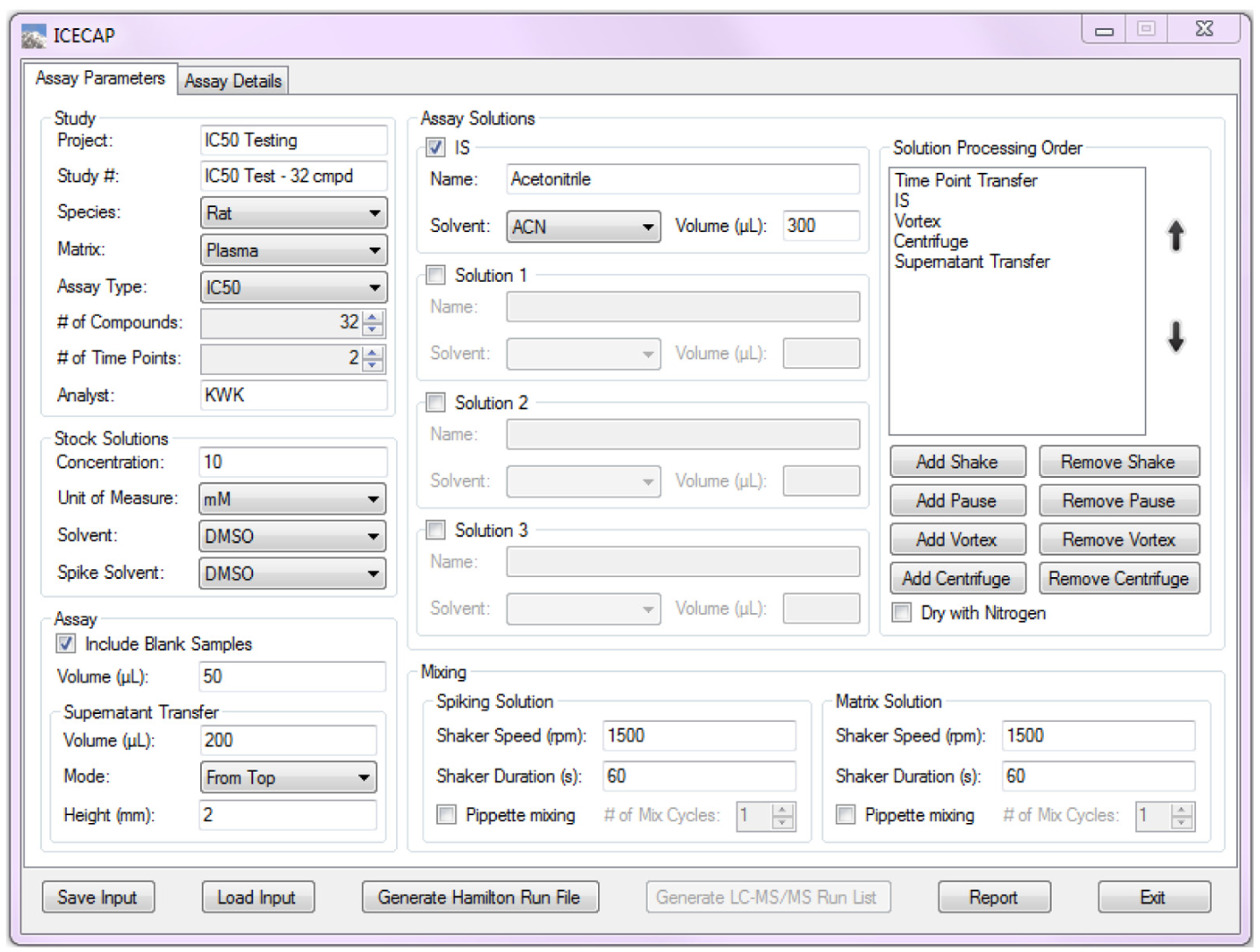
Graphical User Interface Assay Parameters Input.

Figure 2 shows the second GUI input page, where more experimental details could be specified. The number of time points specified in the first GUI page becomes editable in groups of five in the Time Points group box. The wells corresponding to the number of compounds specified in the first GUI page are activated for input in the Compound Stock Plate Map group. Compound names input here are used in the Hamilton run file, sample sequence list, and final report. In the Matrix Solution Preparation group box, the volume percentage of spiking solution in the final matrix solution (p value) is an important user input parameter that would affect the solution preparation scheme computation. The spiking volume percentage is limited to be between 0.5% and 5%. The user-specifiable number of matrix solution concentration levels ranges from 6 to 10. The lower limit of 6 is the very conservative minimum data points needed to capture a fully developed IC₅₀/EC₅₀ curve.²⁰ The upper limit of 10 is due to the 96-well plate layout (vide infra) limitation. One of three ways of specifying the matrix solution concentrations needs to be selected. In the first way, the highest matrix solution concentration and the dilution factor between any two concentration levels are specified. This is the most commonly used approach because in typical IC₅₀/EC₅₀ dose–response curves, the dose (x-axis) is presented in logarithm scale. A fixed dilution factor between any two concentration levels produces evenly spaced x values on the logarithm scale. In the second way, the lowest and the highest concentrations are set. Values in between are computed automatically, and the dilution factor is shown as a read-only value. This approach also produces evenly spaced x values in the dose–response curve. In the third way, input fields corresponding to the number of concentration levels are activated for user input of any concentration levels desirable. These matrix solution concentration input options offer maximum flexibility and encompass all practical IC₅₀/EC₅₀ dose preparation needs. In the Email Notifications group box, users have the option to have the system send out notification emails when a run needs operator attention.

Figure 2.

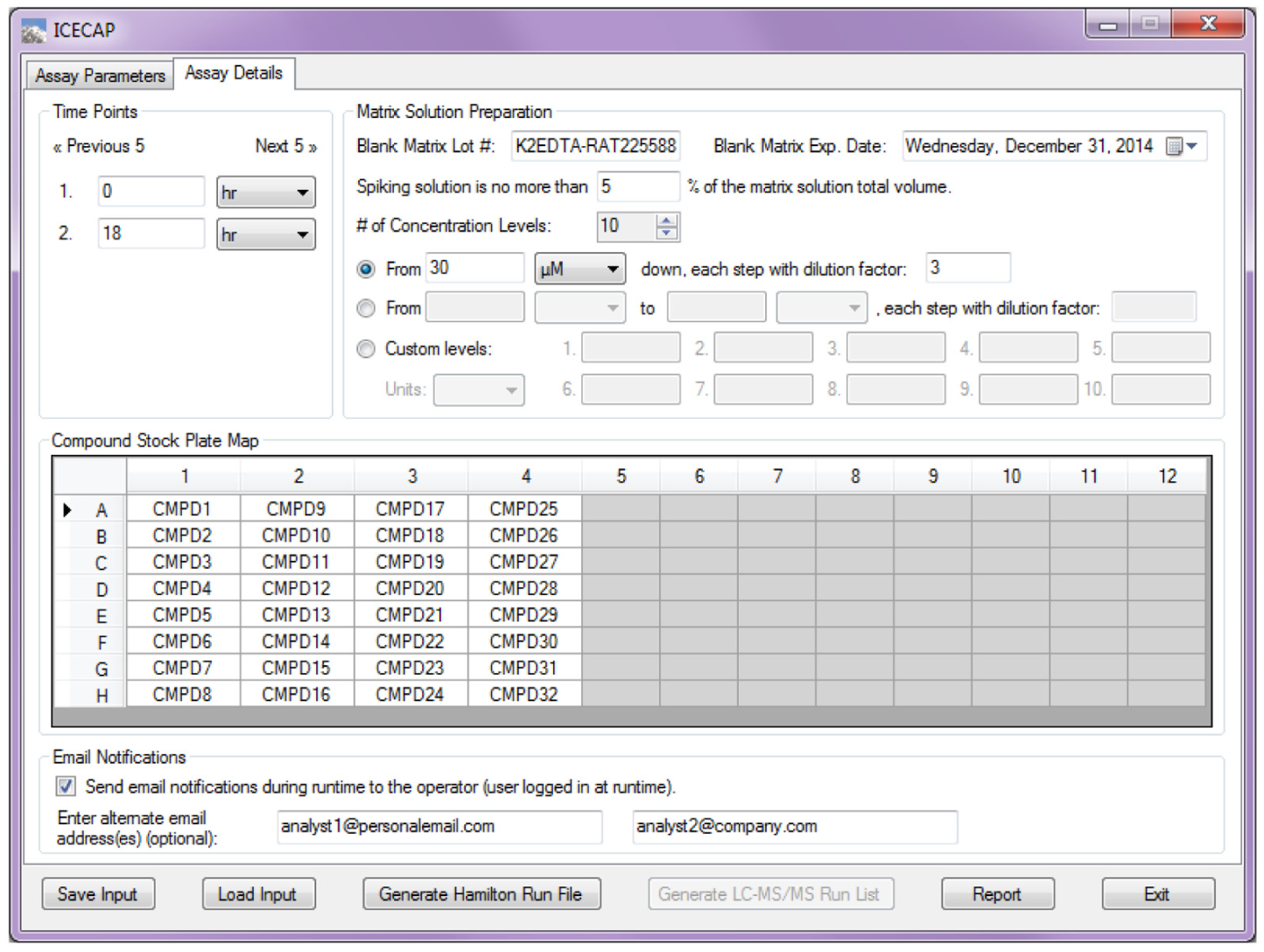
Graphical User Interface Assay Details Input.

Internal Computation

Experimental design input by users only sets the framework and goal of the experiment. To actually carry out the experiment, many more experimental details need to be worked out before starting. ICECAP uses a much more comprehensive parameters list in addition to user input to describe the experiment ( Table 1 ). In Table 1 , parameters shown in bold are user input; parameters in italic could be either user input or calculated. The rest are used for internal computation.

Table 1.

Parameters Used for ICECAP Internal Computation.

C_stock – concentration of the stocks; same for all compounds

C_1m – the first (lowest) matrix concentration

C_nm – the last (highest) matrix concentration

C_1s – the first (lowest) spiking concentration

C_ns – the last (highest) spiking concentration

C_int – concentration of intermediate spiking solution

V_assay – assay volume

n – concentration levels (nonzero)

N_t – number of time points, including time 0

p – percentage of spike solution volume in total matrix solution volume

DF_s1 – dilution factor from stock to intermediate spiking solution

DF_s2 – dilution factor from intermediate spiking solution to highest concentrated spiking solution

DF_s2m – dilution factor from spiking solution to matrix solution

DF_step – step dilution factor (from concentrated to less concentrated)

DF_max – maximum dilution factor in one step, set to 1000 µL/5 µL = 200

V_m – volume of final matrix standard solution (same for all concentration levels)

V_safety – safety volume, set at 100 µL

V_s2m – volume of spiking solutions to be transferred to prepare matrix standard solutions

V_mblank – volume of blank matrix needed to prepare a matrix standard solution

V_s – volume of minimum spiking solution to prepare

V_1s – volume of first (lowest concentration) spiking solution to prepare

V_ns – volume of last (highest concentration) spiking solution to prepare

V’_2s – volume of second lowest concentration spiking solution needed to prepare the 1s

V_2s – total volume of second lowest concentration spiking solution to prepare

V’_ns – volume of the highest concentration spiking solution needed to prepare (n−1)s

V_ns – total volume of highest concentration spiking solution to prepare

V_stock2ns – volume of stock solution needed to prepare highest concentrated spiking solution

V_stock2int – volume of stock needed to prepare intermediate spiking solution

V_int2ns – volume of intermediate spiking solution to be transferred to highest concentrated spiking solution

V_blank2ns – volume of blank solvent needed to prepare highest concentrated spiking solution

V_int – volume of intermediate spiking solution to prepare

V_int2ns – volume of intermediate spiking solution to transfer to highest concentrated spiking solution

V_blank2int – volume of blank solvent needed to prepare intermediate spiking solution

Bold are user input; italic are either input or calculated; the rest are only used in internal computation.

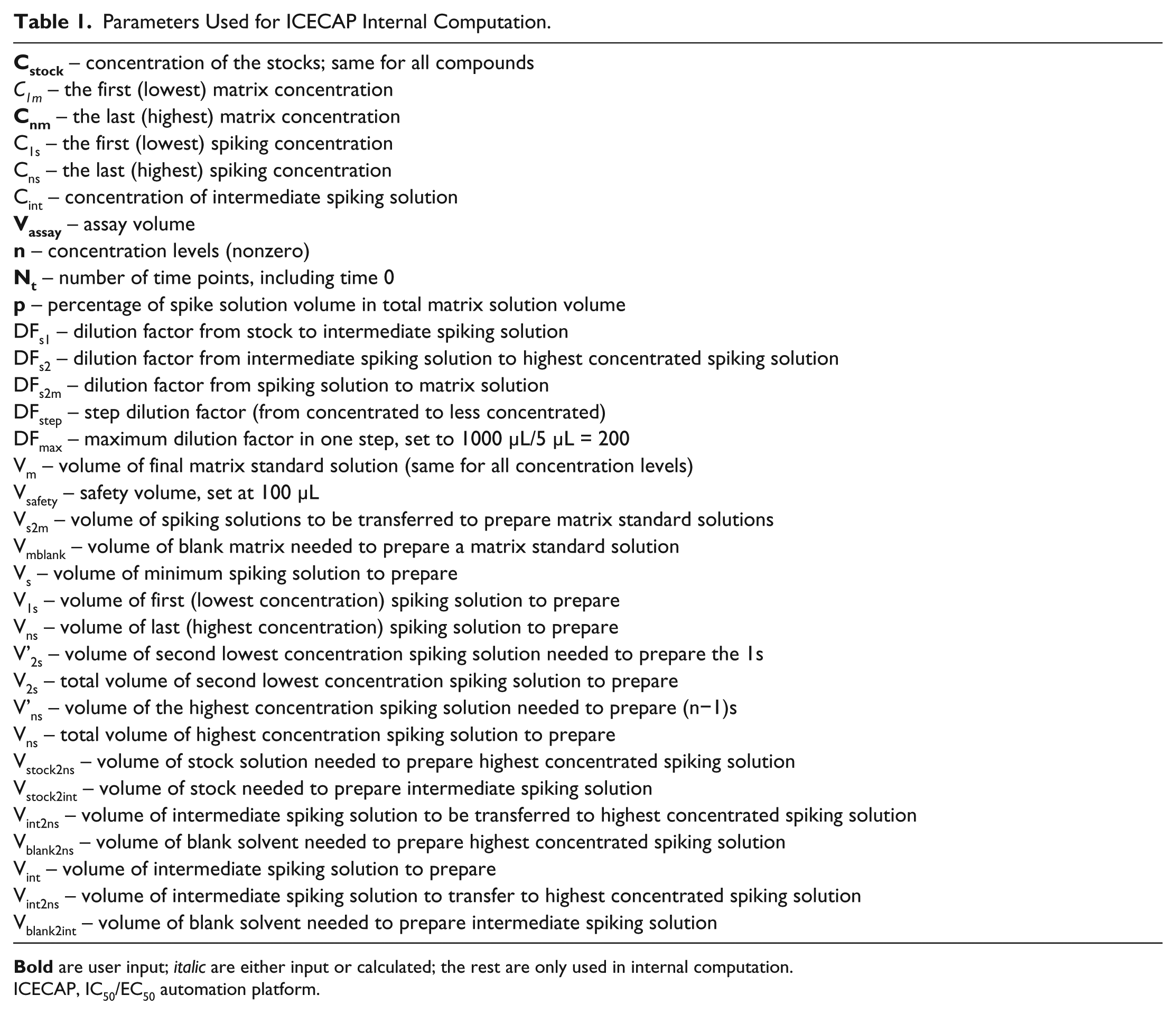
ICECAP, IC₅₀/EC₅₀ automation platform.

The internal computation process starts with validation of user input ( Fig. 3 , section II). For example, ICECAP has an empirical global minimum liquid handling volume of 5 µL (using 10 µL tips) and maximum liquid handling volume of 1000 µL (using 1000 µL tips). Therefore, the maximum single-step dilution factor is 200. ICECAP allows one intermediate solution. Thus, the maximum dilution ICECAP can achieve from weighing stock solution to highest concentration spiking solution is 200 × 200 = 40,000. From spiking solutions to matrix solutions, there is another maximum dilution factor of 200. So the overall maximum dilution factor from weighing stock solution to highest concentration matrix stock is 8,000,000. The ICECAP GUI enforces the rule.

Figure 3.

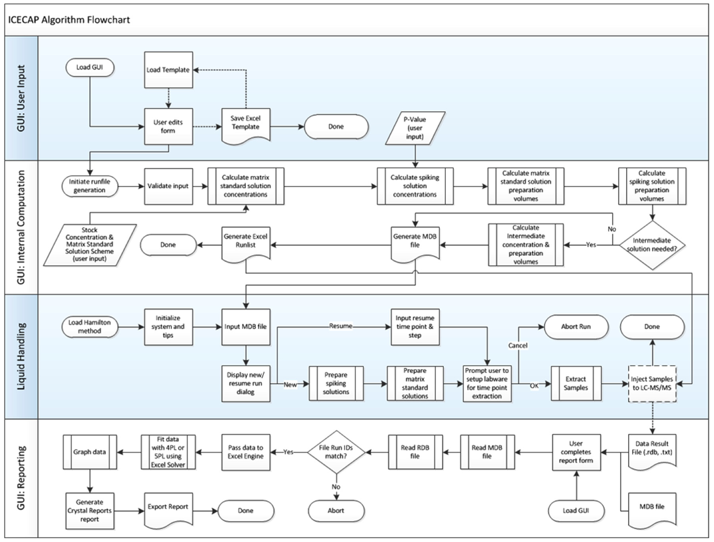
Algorithm Flowchart.

After all validation is done, all target matrix solution concentrations are computed first using the user-specified approach ( Fig. 2 ). Then, using the user input value p, corresponding spiking solution concentrations are computed. The empirical global minimum liquid handling volume 5 µL is 0.5% of 1000 µL, which is why the lowest allowable p value is set at 0.5% (vide supra). With both matrix and spiking solution concentrations known, the matrix solution preparation scheme is then computed, taking into consideration the global minimum liquid handling volume, safety volume (to avoid liquid handling errors), and total matrix solution volume needed for all time point experiments. Next is the spiking solution preparation scheme computation, which starts at the lowest concentration level and progressively up. In each cycle, the volume needed for actual use is combined with the safety volume needed to avoid liquid handling errors when computing the volume needed coming from the next higher concentration solution. When reaching the highest concentration spiking solution, if an intermediate solution is needed, its preparation scheme is computed as well. All user input and computation results are stored in a Microsoft Access database *.mdb file, which has four tables in it: an assay parameters table ( Fig. 4 ); a calculations table of all computation results; a matrix solutions table of concentrations, dilution factors, and preparation volumes; and a spiking solutions table with detailed information on spiking solution preparation, such as source and target lab ware and positions, preparation volume, and so on. A sample list is then exported into a Microsoft Excel file ( Fig. 5 ) for sample analysis purposes.

Figure 4.

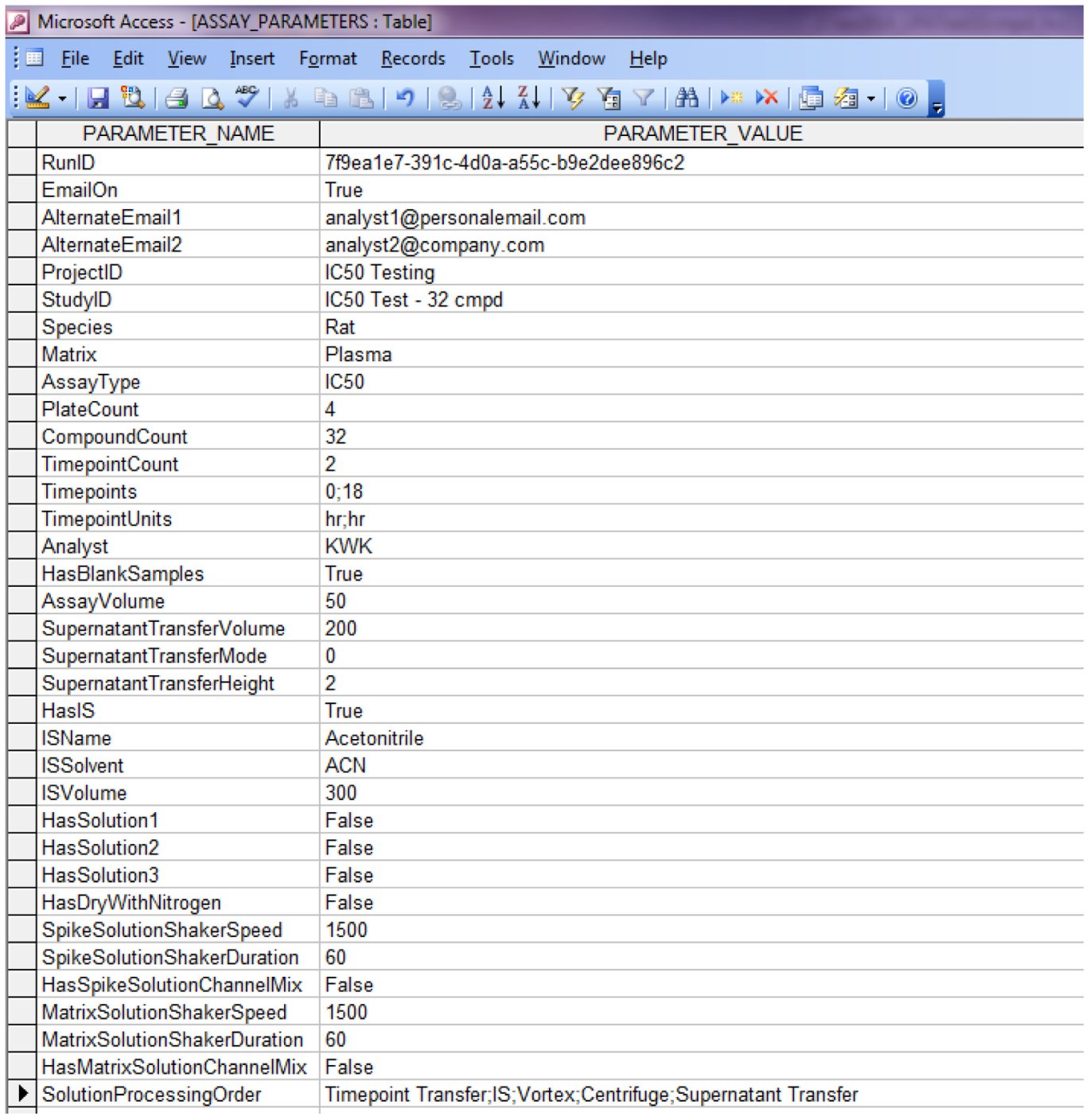
Hamilton Run File Assay Parameters Table.

Figure 5.

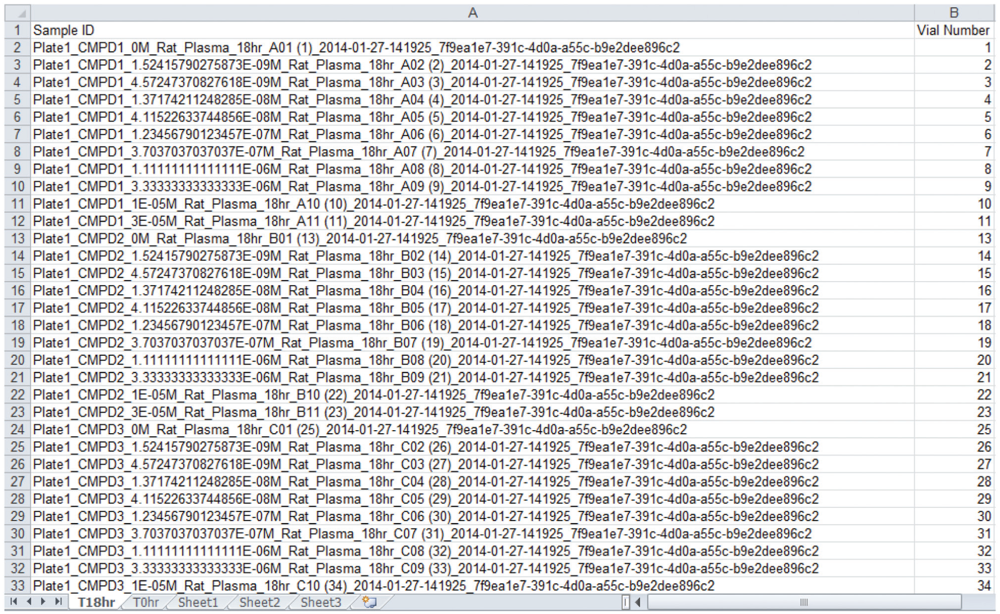
Sample Analysis Sequence List.

ICECAP Hamilton Script Program

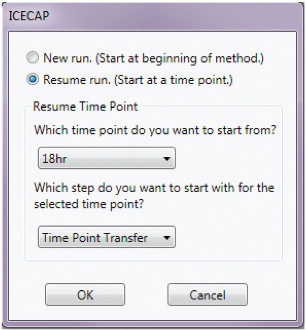
The ICECAP Hamilton script ( Fig. 3 , Section III) was developed in Venus 2.0 and executes on the Hamilton MicroLab STAR robot to carry out spiking solution preparations, matrix solution preparations, and sample extractions after incubation. After system initialization and taking the Access database file, it prompts the user to decide the program flow: whether to start a new run from the beginning or to resume a run at specific time points ( Fig. 6 ). 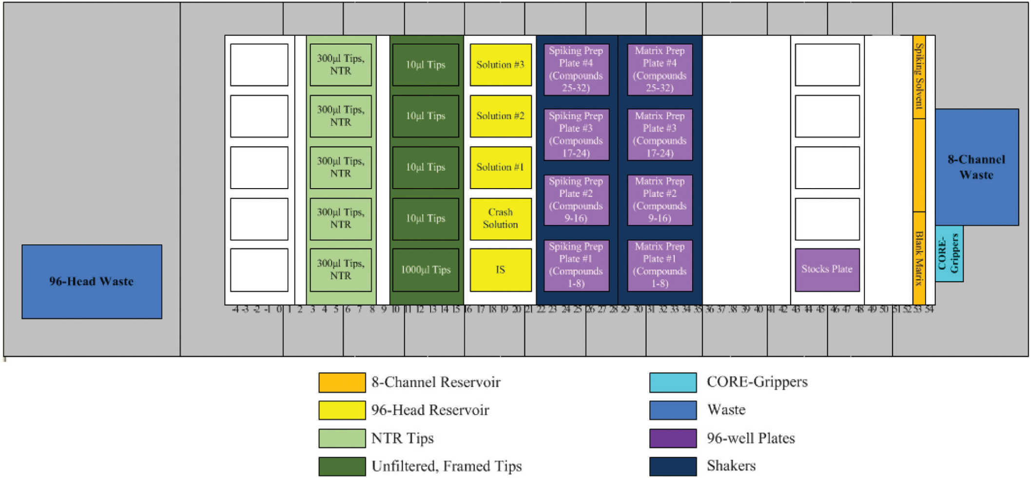If it’s a new run, the program starts from spiking solution preparation, followed by matrix solution preparation. There are 2×4 integrated shakers on the MicroLab STAR extended deck: 4 for spiking solutions and 4 for matrix solutions ( Fig. 7 ). 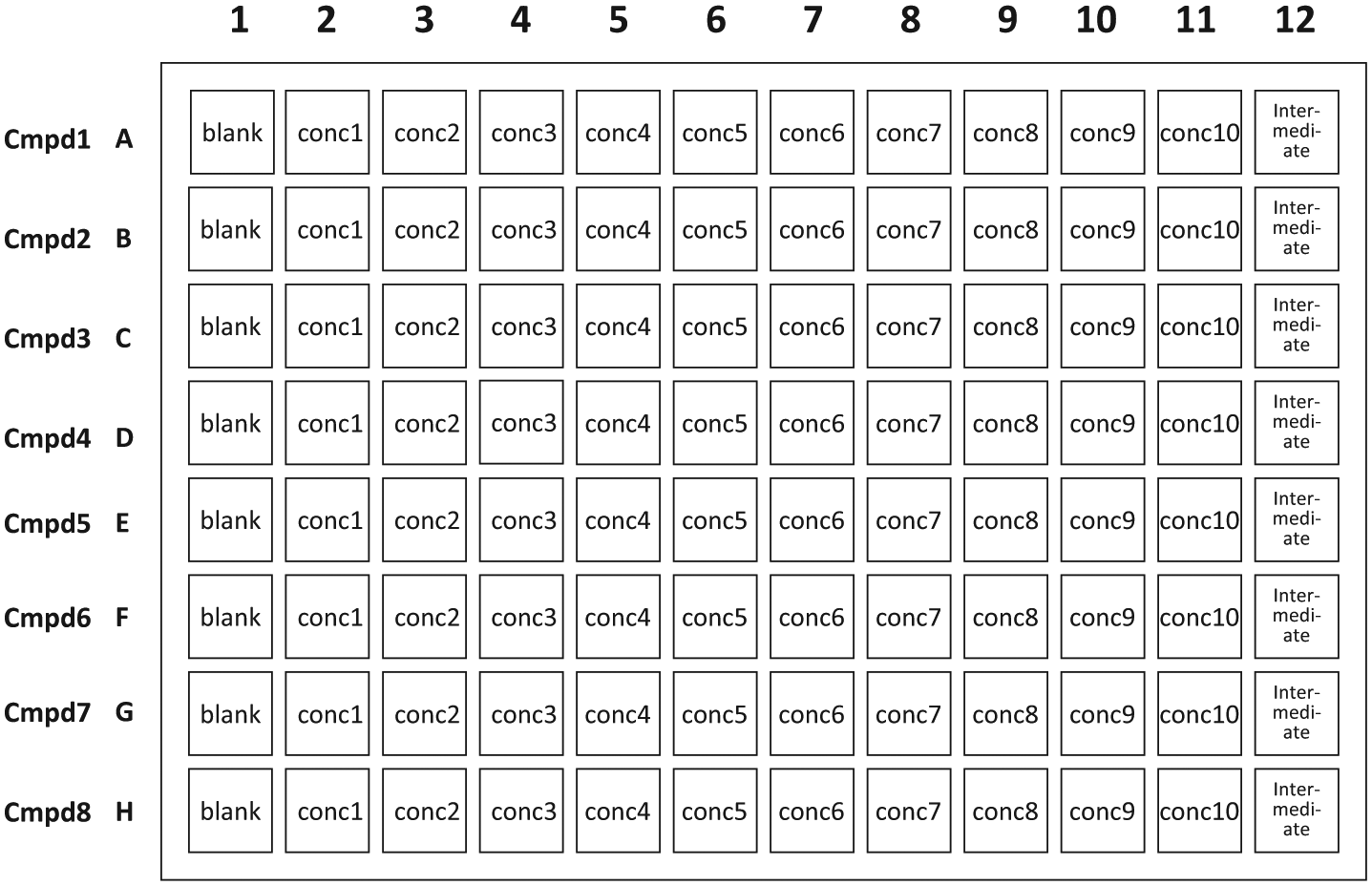Considering the deck space needed for other solutions, tips, and reservoirs, and the fact that both spiking and matrix solutions preparations need shaking, this is about the maximum number of shakers that could be accommodated on a single robot without further sacrificing plate space (i.e., four shakers take up five 96-well plate spaces and are wider than a normal plate carrier). Each plate can handle eight compounds up to 10 concentration levels ( Fig. 8 ). Therefore, ICECAP can process up to 32 compounds per run. If time 0 sample processing is requested along with the new run, immediately after matrix solutions preparation, the Hamilton program will pause and prompt the user to set up the deck before time 0 sample extraction would take place (Suppl. Fig. 1). If the run is a time point resume of a previous run ( Fig. 3 , Section III), the Hamilton program will display a similar message (Suppl. Fig. 2) and prompt the user to get everything ready before sample extraction (Suppl. Fig. 1).

Figure 6.

Hamilton Program Flow Selection.

Figure 7.

Hamilton Deck Layout for Spiking and Matrix Solution Preparations.

Figure 8.

Typical Spiking and Matrix Solution Plate Map.

Experimental

ICECAP testing follows this process: First, the GUI program was tested for enforcement of business and validation rules, and correct output of the Access file tables and the sample analysis sequence list. Then, the Hamilton script was tested in simulation mode, the trace file of which was closely examined to ensure the absence of programming logic errors. On the Hamilton deck, the first liquid tested was tap water dyed with food color to check that dilution was happening, followed by real blank solvents tests to ensure liquid classes were appropriate such that no dripping was occurring during liquid transfers.

When all of the above tests passed successfully, the system was used in a series of real studies to perform IC₅₀ experiments, and the results were compared with manually obtained ones. The background of the real studies involves autotaxin, an enzyme that catalyzes lysophosphatidylcholine (LPC) to lysophosphatidic acid (LPA) conversion.^21–25 Compounds were screened to evaluate their autotaxin enzyme inhibition potency (IC₅₀ values). Experimental endpoint was the measurement of biomarker LPA (20:4 and 18:1) concentrations in rat plasma.

Materials

Compounds 1 through 4 and compound internal standard (IS) were internally synthesized. 18:3 LPA was from Echelon Biosciences (Salt Lake City, UT); 17:0 LPA was from Avanti Polar Lipids Inc. (Alabaster, AL); ammonium formate was from Sigma-Aldrich (St. Louis, MO); pooled rat plasma (lots RAT225586 and RAT225588) were from Bioreclamation (Westbury, NY); high-performance liquid chromatography (HPLC)-grade methanol and acetonitrile were from Fisher Chemical (Hampton, NH); 99% formic acid was from Acros Organics (Fisher Scientific, Hampton, NH); 2 mL 96-well plates were from Analytical Sales and Services (Pompton Plains, NJ); and 96-head Nalgene polypropylene solvent reservoirs were from Fisher Scientific (Hampton, NH). HPLC columns used were ACE 3.0 µm 50×2.1 mm C18-AR from Mac-Mod Analytical (Chadds Ford, PA), and Atlantis 5.0 µm 50×2.1 mm HILIC Silica from Waters (Milford, MA). Compound mobile phase A was 0.1% formic acid in 95:5 water–acetonitrile; compound mobile phase B was 0.1% formic acid in 50:50 acetonitrile–methanol. LPA mobile phase A was 10 mM ammonium formate in water; LPA mobile phase B was 10 mM ammonium formate in 95:5 acetonitrile–methanol.

Instruments and Liquid Chromatography–Tandem Mass Spectrometry (LC-MS/MS) Methods

The Hamilton MicroLab STAR liquid handling robot was running Venus 2.0 robot control software and was equipped with eight vendor integrated INHECO shakers. Three types of conductive, disposable tips were used: 10 µL and 1 mL tips were in ordinary racks, whereas 300 µL tips were in nested tip racks ( Fig. 7 ).

Quantitative analyses of both compounds and LPA were carried out using the same LC-MS/MS system. The triple quadruple mass spectrometer was Applied Biosystems (Carlsbad, CA) Sciex API 5500 running in ESI+ mode for compounds and ESI− mode for LPAs. The HPLC system used was Shimadzu Prominence LC-20AD XR pumps with SIL-20 AC XR Prominence refrigerated autosampler and rack changer. Prior to running ICECAP experiments, LC-MS/MS methods for compounds 1–4, compound IS, and all LPAs were first manually optimized using neat solutions. MRM transitions for compounds, compound IS, and the LPAs were listed in Table 2 . Compounds quantitation was conducted on the ACE column with the following optimized HPLC gradient: 0.01–0.5 min 40% B; 1.9–2.4 min 95% A; 2.5–3.0 min 40% B; and run time was 3.0 min. LPA analyses were conducted on the Atlantis column with the following optimized HPLC gradient: 0.01–0.5 min 100% B; 1.9–2.4 min 40% A; 2.5–3.0 min 100% B; and run time was 3.0 min. Ion chromatogram peak integrations were carried out with Analyst version 1.6.2.

Table 2.

MRM Transitions for Compounds, IS, and LPAs.

Name	Mol. Mass	Q1	Q3
Compound IS	543.548	544.3	375.1
Compound 1	543.548	544.3	389.1
Compound 2	451.323	452.1	434.1
Compound 3	491.594	492.3	349.1
Compound 4	513.948	514.2	443.1
20:4 LPA	475.556	457.4	153.1
18:1 LPA	458.502	435.4	153.1
18:3 LPA (IS)	476.45	431.4	153.1
17:0 LPA (IS)	446.491	423.3	153.0

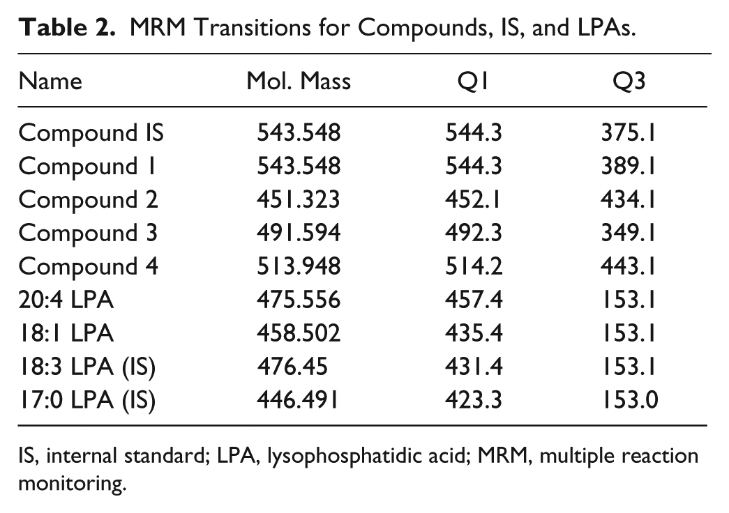
IS, internal standard; LPA, lysophosphatidic acid; MRM, multiple reaction monitoring.

Sample Procedures

ICECAP handles three wet chemistry experimental types: spiking solution preparation, matrix solution preparation, and sample extraction. Spiking solution preparations follow their preparation schemes saved in the Microsoft Access database file and usually use serial dilutions from the concentrated stock, with the help of one possible intermediate solution. Whenever possible, eight-channel parallel processing is used to improve system throughput. Matrix solution preparations also follow the preparation scheme saved in the Microsoft Access database file, but in general are done using the 96 CORE head to boost throughput.

For compounds’ sample extractions in the test experiment, at time zero, 300 µL of IS (100 ng/mL of compound IS in ACN) was added to 50 µL of samples, then capped, vortexed, and centrifuged. 25 µL of supernatant was mixed with 500 µL water; 5 µL was injected for analysis. Supplementary Figures 3–5 are a representative compound and IS chromatogram, IS trace, and calibration curve. For LPAs, after 18 h of incubation at 37 °C, 300 µL of IS (500 ng/mL of 18:3 and 17:0 LPA in ACN) was added to 50 µL of samples, then capped, vortexed, and centrifuged. 200 µL was transferred, 5 µL was injected for analysis. Supplementary Figures 6 and 7 are representative LPA and IS chromatograms and IS trace.

ICECAP Workflow and Data Flow

Figure 9 is the workflow and data flow diagram. ICECAP GUI input could be manual (step 1a). To save time, the input could also be saved to a template (step 1b) for later retrieval (step 1c). After saving the Microsoft Access database file (step 2), the Generate LC-MS/MS Run List button on the GUI would be activated, allowing users to save (step 3) a LC-MS/MS run sequence file like the one in Figure 5 . The Access database file is manually input to the ICECAP Hamilton script for execution (step 4). While that is happening, users would use the LC-MS/MS run list to set up the LC-MS/MS analyses batch and the like on the LC-MS/MS system (step 5). After sample extractions are done, the extracted plates are analyzed on the LC-MS/MS (step 6). Ion chromatogram peak integration results are saved in *.txt or *.rdb format (step 7), then fed into the ICECAP GUI (step 8a) along with the original Access database file (step 8b) for nonlinear regression curve fitting, IC₅₀/EC₅₀ values computation, and experimental report generation (step 9).

Figure 9.

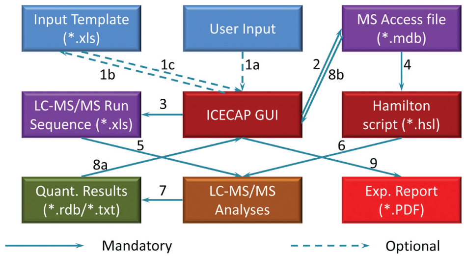
Workflow and Data Flow.

Results and Discussions

System Performance

ICECAP performance testing was aimed at addressing the following key points: quality of the matrix solution preparation automation, quality of built-in nonlinear regression curve fitting functions, and overall system performance compared to manual experiments (i.e., the correlation between EC₅₀ or IC₅₀ values obtained through ICECAP versus manual experiments).

Matrix solution preparation quality

To test the performance of ICECAP liquid handling functions, time zero matrix samples were aliquot and processed using the compound extraction procedure, and analyzed on the LC-MS/MS for compound concentrations. Eight replicates of manually prepared compound 1 matrix curves were used as standards (STD), and eight replicates of ICECAP prepared matrix samples were used as QCs. Table 3 is a compilation of the STD and QC accuracy and precision. Note that the 30 µM samples saturated the MS detector; therefore, their data are not used. These data demonstrate production-quality liquid handling accuracy and precision [19], and are sufficient for IC₅₀/EC₅₀ screening assays.

Table 3.

Comparison of Compound 1 Manual versus Automated Matrix Sample Preparations.

Concentration	Manual Run (STD)			Automated Run (QC)
nM	N	% CV	% Bias	N	% CV	% Bias
1.52	8	17.2	5.6	8	14.2	11.3
4.57	8	9.5	2.2	8	6.4	2.2
13.7	8	5.4	−2.6	8	6.5	−2.6
41.2	8	5.3	1.8	8	5.7	1.6
123	8	5.2	5.5	8	6.4	1.9
370	8	6.0	−0.1	8	5.0	0.0
1110	8	3.0	0.5	8	6.4	−5.0
3330	8	3.5	1.1	8	3.5	−3.8
10000	8	3.3	−7.6	8	2.8	−11.5

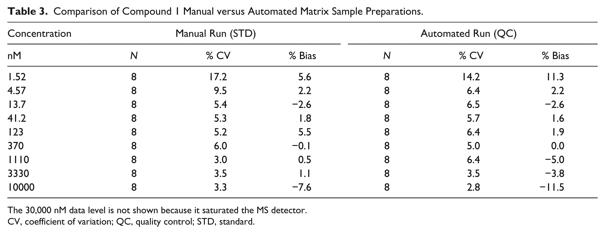
The 30,000 nM data level is not shown because it saturated the MS detector.

CV, coefficient of variation; QC, quality control; STD, standard.

Built-in nonlinear regression curve fitting quality

In a non-high-throughput screening lab, the final IC₅₀/EC₅₀ value is traditionally obtained through a commercial nonlinear regression curve fitting software package such as the GraphPad Prism. Scientists would copy and paste dose and response data into Prism one compound at a time, compute the IC₅₀/EC₅₀ value, then export the value and curve fitting graph into a container file for reporting purposes. Repeated processes like this could easily lead to scientist mental and physical fatigue and error. In ICECAP, this entire process (i.e., getting data, nonlinear curve fitting, and IC₅₀/EC₅₀ value computation, graphing, and reporting) is automated. Figure 10 is the ICECAP report function input form, which takes two files as input. The first is the Microsoft Access file ( Fig. 4 ) of the experiment. The second is the analysis results file. Because Sciex mass spectrometers are our main quantitative analyses instruments and Analyst is their instrument control and data acquisition software, the ICECAP reporting module was coded to be able to read Analyst results files (*.rdb) directly through its application programming interface (API). This eliminates one additional step of copying and pasting, and the potential clerical errors associated with it, and significantly improves data processing throughput (vide infra). To achieve automated data processing, the same mechanism reported in the literature²⁶ was used to encode or decode sample IDs. All experimental details about any particular sample, such as plate number, compound name, concentration, matrix, time point, well position on the 96-well plate, time stamp, and that experiment’s global unique identifier (GUID), were encoded into that sample’s name ( Fig. 5 ). The Microsoft Access file is also tagged with the same GUID ( Fig. 4 ). The ICECAP reporting algorithm reads the Access file (*.mdb) and the results file (e.g., Analyst *.rdb file), and would only proceed when their respective GUIDs match ( Fig. 3 , Section VI). This mechanism ensures correct reporting of experimental results each time. After decoding the sample IDs and analyses results into data table, ICECAP passes data to the Microsoft Excel Solver engine to conduct nonlinear regression curve fitting²⁷ using either the four-parameter logistic (or Sigmoidal) equation (4-PL):²⁸

y = B + \frac{T - B}{1 + {(\frac{x}{c})}^{H}}

where y is the response, x is the dose, B is the bottom of the curve, T is the top of the curve, H is the Hill’s slope, and C is the IC₅₀ or EC₅₀ value; or the five-parameter logistic equation (5-PL):²⁹

y = B + \frac{T - B}{{(1 + {(\frac{x}{c})}^{H})}^{A}}

where A is the asymmetry factor. 5-PL reduces to 4-PL when A = 1. On the reporting GUI ( Fig. 10 ), users can choose one of the above two curve fitting equations, along with response type (peak area or peak area ratio) and graph y-axis type (absolute or relative³⁰). The “no dose response” (NDR) cutoff is a user-specified value of the percentage change of response from the top to the bottom of the curve, at less than which the experiment would be reported as NDR.²⁷ The outlier cutoff is a user-defined value of the difference between experimental data and curve fitting data, beyond which the data point would be marked in the data table as an outlier.²⁷ Curve fitting results and graphs are passed into Crystal Reports for report generation ( Fig. 3 , Section IV). 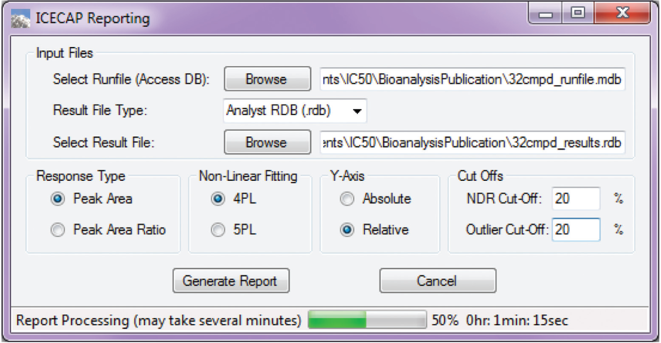A complete ICECAP report consists of assay information, the extraction procedure (Suppl. Fig. 8), reporting (parameters) information, a curve fitting results compilation, a graph for each curve (Suppl. Fig. 9), a data summary table, and plate maps of source compound, spiking, and matrix plates.

Figure 10.

Graphical User Interface Report Input.

To compare the ICECAP built-in nonlinear regression curve fitting algorithm results with those obtained through GraphPad Prism, one ICECAP experiment’s dose–response data set of eight replicates of compound 1 was processed in two ways respectively (both using the 4-PL equation): through ICECAP’s Analyst API and built-in nonlinear regression curve fitting algorithm, as well as manually through copying and pasting data into GraphPad Prism 6.0.1. Table 4 is the comparison of the results. As demonstrated in the table, the percentage difference of the IC₅₀ values obtained through ICECAP and GraphPad Prism is small enough that ICECAP’s built-in nonlinear regression curve fitting algorithm can function as a replacement of GraphPad Prism.

Table 4.

ICECAP versus GraphPad Prism 4-PL Algorithm Comparison Using Compound 1 Robot Run Data.

	20:4 LPA IC₅₀ Values (µM)
	n	Average	% CV	% Difference
GraphPad Prism	8	0.1185	29.2	0.2
ICECAP		0.1188	29.2

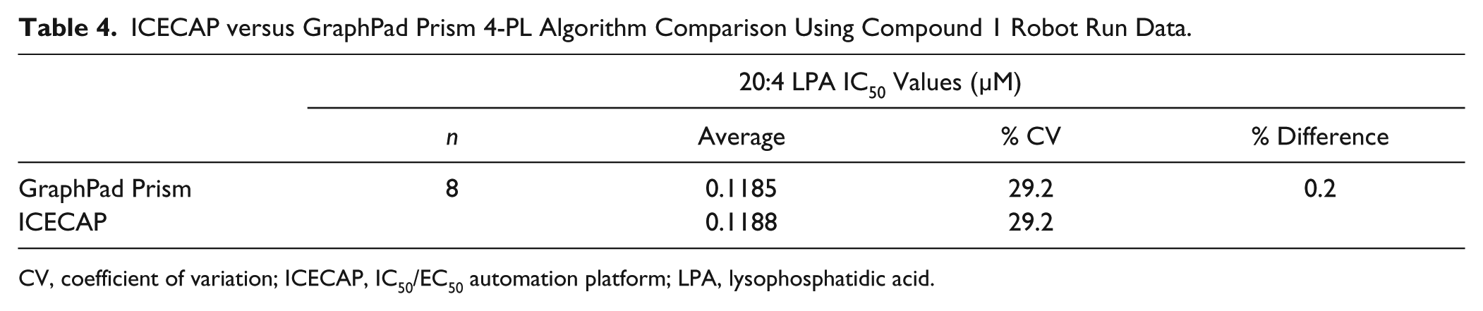
CV, coefficient of variation; ICECAP, IC₅₀/EC₅₀ automation platform; LPA, lysophosphatidic acid.

Manual vs. ICECAP comparison

To test the overall performance of ICECAP versus manual IC₅₀ experiments, the following experiments were conducted: eight replicates of compound 1 were processed automatically through ICECAP and used its built-in data processing algorithm for IC₅₀ values; another eight replicates were processed manually (sample extraction, incubation, and the LC-MS/MS analyses were done in the exact same procedure as the automated ones) and used GraphPad Prism to obtain IC₅₀ values. These two sets of IC₅₀ values were compared in Table 5 . As demonstrated in the table, IC₅₀ values obtained through ICECAP correlate well with manually obtained ones, and so ICECAP is performing as expected.

Table 5.

ICECAP versus Manual Experiment Comparison for Compound 1.

		20:4 LPA IC₅₀ Values (µM)
Experiment	Curve Fitting	N	Average	% CV	% Difference
Robot Run	ICECAP 4PL	8	0.1188	29.2	8.5
Manual Run	Prism 4PL	8	0.1092	37.5

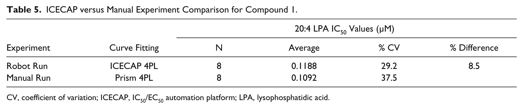
CV, coefficient of variation; ICECAP, IC₅₀/EC₅₀ automation platform; LPA, lysophosphatidic acid.

Messaging

A desired feature of bioanalytical wet chemistry automation is minimum user attendance at the robots. To reduce operator attendance at the robot, the integration of small hardware accessories—for example, capping, vortex, centrifuge, and decapping—into the existing robot platform would be desirable. However, with the current robot hardware, this is still done case by case instead of as the norm. Therefore, even though most of the wet chemistry steps of an assay are automated in existing systems, there would still be sparing offline steps that are not automated and need manual intervention. The timing of these steps during an automated run varies from assay to assay. To free up users as much as possible for other intellectual tasks, system messaging capability is being added into ICECAP to only alert users when the robot needs manual intervention. To achieve this, operators’ email addresses are first collected through either their corporate network login, which is tied to the enterprise active directory, or user input of alternative email addresses ( Fig. 2 , bottom) before the automated run starts. During the execution of robotic scripts, just before each message box pops up prompting users for manual intervention, such as the one shown in Supplementary Figure 2, scripts are put in place to tap into the user enterprise’s messaging [outgoing Simple Mail Transfer Protocol (SMTP)] server to send a short reminder message (Suppl. Fig. 10). With the proliferation of smart phones and the ease of access to enterprise and/or personal emails, this messaging mechanism enables the operator to walk away from the robot to perform other tasks after an automated ICECAP run starts, and only come back when they receive alert emails.

System Flexibility

Several features of ICECAP make it a versatile IC₅₀/EC₅₀ automation platform. First is the flexible input of target matrix solution concentration levels ( Fig. 2 ). In most IC₅₀/EC₅₀ experiments, concentration levels of adjacent doses follow a fixed dilution factor pattern such that the final dose–response semilogarithm plot will have a data set evenly distributed across the x-axis. However, the exact concentration range that would capture the fully developed response curve (determined by the starting concentration and subsequent dilution factors) could vary from compound to compound. This change, if done manually, requires meticulous recalculation of the matrix solution preparation scheme and, throughout time, becomes a burden. Also, there might be times when unevenly distributed doses are desired to capture the top or bottom plateau of the curve. ICECAP’s flexible matrix concentration input capabilities ( Fig. 2 ) make these changes effortless.

Second is the flexible solution processing order. IC₅₀/EC₅₀ sample processing details such as solution type, volume, and order of addition could vary from assay to assay. ICECAP encapsulates all of the above into its algorithm ( Fig. 1 ) and supports unlimited variations of those details.

Third is that sample analysis is not limited to LC-MS/MS only. Because ICECAP outputs encoded sample IDs in sample analysis sequence lists, and decodes and processes quantitative data using those sample IDs, the actual quantitative analysis method does not matter as long as the returned data contain those sample IDs.

Fourth is the experimental resume function ( Fig. 6 ). A large portion of any IC₅₀/EC₅₀ experiment is incubation, which is typically overnight. Even though incubator hardware could be integrated with existing robots, and the incubation step automated, that route was not taken because it was deemed inefficient. Instead, the resume algorithm was implemented to free up the robot for other applications during the long IC₅₀/EC₅₀ incubation period. We believe this is a better use of the capital equipment.

System Throughput Improvement

To gauge ICECAP’s full capacity, a 32-compound run was performed in the 4×8 fashion: each of the four plates consists of eight replicates of the same compound (1–4), respectively ( Fig. 8 ). Manual preparation of the spiking solutions of all four plates, manual spiking into the blank matrix, and the manual sample extraction procedures would take an average bioanalyst at least a full working day (and possibly longer) to complete, in addition to the preparation scheme design. With ICECAP, all of the above was done in less than 2 h, thanks to the eight-channel parallel processing of the compounds’ spiking solution preparation and the 96-well simultaneous handling of spiking and sample extractions ( Fig. 8 ).

In manual IC₅₀/EC₅₀ experiments, copying and pasting the data into Excel for graphing, copying and pasting data into GraphPad Prism for IC₅₀/EC₅₀ value calculation, and putting together everything in a report take our analyst at least 2 min per compound on average, with possibilities for analyst clerical error. For 32 compounds, the manual process would take at least 1 h to finish. In ICECAP, with GUID implementation, direct data retrieval through Analyst API, plus built-in nonlinear regression curve fitting capabilities, running a guaranteed error-free 32-compound report (4-PL nonlinear regression curve fitting, graphing, and reporting) on an ordinary office laptop (Intel Core i5-3320M CPU: 2 cores, 4 logical processors, 2.60 GHz, 4 GB RAM) under Windows 7 Enterprise edition took only 3 min and 23 s.

Conclusions and Future Perspectives

Until commercial turnkey automation solutions are readily and widely available, there are needs, and it is value added to customize general-purpose robots and make them easier to use for targeted applications. While doing so, many labs do piecemeal automation, that is, they automate and perfect one step or a few steps of the workflow to achieve high throughput to the extreme while neglecting the interconnection, the interoperation of those disparate automation silos and pieces, and the usability, which results in poor user experiences. What we have been doing here is to integrate those individual automation pieces into a user-friendly automation solution.

ICECAP provides a general-purpose automation platform for non-high-throughput screening labs when conducting IC₅₀/EC₅₀ assays. Its flexible matrix solution concentration levels designation and concentration values input, flexible solution processing order, automated computation of liquid handling schemes, and automation-assisted parallel processing of wet chemistry procedures can handle the majority of IC₅₀/EC₅₀ assay situations. Its automated data extraction, nonlinear regression curve fitting, and reporting functions greatly improve data-processing efficiency. The combination of wet chemistry automation and data-processing automation capabilities improves IC₅₀/EC₅₀ assay productivity tremendously. Although, strictly speaking, each of the individual automation pieces in ICECAP may not be “new” per se (i.e., they have been published before), the integration of all those approaches and pieces into a general-purpose IC₅₀/EC₅₀ automation platform is new, as far as we know.

Like previous systems,^19,26 ICECAP uses a GUI program plus robot script approach to achieve automation, and it separates user input verification, business logic, liquid handling error prevention algorithms, and liquid handling scheme computation from actual liquid handling logic. The GUI program can be seen as the abstraction layer, and the robot script the execution layer. The link between the two layers is a parameters file, which, for all practical purposes, could be Microsoft Access, Excel, or other common file types. This design of separated abstraction and execution layers inherently makes the system’s rapid retargeting onto other robotic platforms possible: As long as a new robot-specific scripting environment supports the above common file types as input, and the said new robot platform has all the equivalent liquid handling functionalities as the original robot the system was developed on, then new robot-specific scripts could be developed relatively quickly following the same modular design as the original robot script. This saves much development resources and time when porting the application to other robotic platforms.

Because IC₅₀/EC₅₀ assays are for screening purposes, current ICECAP sample extraction functionalities were designed to handle simple sample extractions only. This fit-for-purpose approach suits our current needs. However, as more complex biomarker assays are developed, sample handling requirements might change, which might necessitate more advanced sample extraction automation capabilities. ICECAP could certainly be improved in that area.

Another area of improvement would be use of better nonlinear regression curve fitting algorithms. There are commercially available software components with optimized algorithms tailored for nonlinear regression curve fitting purposes.³¹ ICECAP could integrate those software components and make nonlinear regression curve fitting even faster.

Finally, if we examine the general approach of ICECAP closely, many of the ICECAP ideas such as flexible spiking solutions preparation through serial dilutions, spiking of compounds into blank matrix, flexible solution processing order, flexible selection of resume time points of experiments, automated data processing, and so on are directly applicable to assorted ADME binding–stability–inhibition screening assays as well, with the help of respective special-purpose lab ware in a 96-well format. This clearly points to algorithm reuse. Conceivably, existing ICECAP core programs could be expanded to include those assay types to form a time point assay suite. That would be yet another class of assays that could be automated on the same robotic liquid handling platform.^19,26 If the all-in-one, so-called “bioanalytical wet chemistry kiosk”^32,33 were a mountain to be conquered, then we would be another step closer to the pinnacle covered with the ice cap.

Key Terms

active directory – A directory service implemented by Microsoft to authenticate and authorize all users and computers in a Windows domain type network, for example assigning and enforcing security policies and installing or updating software.

Crystal Reports – Business intelligence application used to design and generate reports from a wide range of data sources. Crystal Reports was bundled with Microsoft Visual Studio .NET 2003–2008, and was available as an add-on software for Visual Studio .NET 2010.

application programming interface (API) – A protocol intended to be used as an interface by software components to communicate with each other. Sciex Analyst API includes specifications for their proprietary *.rdb and *.wiff files’ data structures.

globally unique identifier (GUID) – a unique reference number used as an identifier in computer software, stored as 128-bit values and commonly displayed as 32 hexadecimal digits with groups separated by hyphens.

Simple Mail Transfer Protocol (SMTP) – An internet standard for electronic mail transmission across internet protocol networks. Mail servers use SMTP to send and receive messages, whereas user-level applications use SMTP only for sending messages to mail server for relaying.

Footnotes

Declaration of Conflicting Interests

The authors declared no potential conflicts of interest with respect to the research, authorship, and/or publication of this article.

Funding

The authors received no financial support for the research, authorship, and/or publication of this article.

References

Atkinson

A. J.

Lalonde

R. L.

Introduction of Quantitative Methods in Pharmacology and Clinical Pharmacology: A Historical Overview. Clin. Pharmacol. Ther. 2007, 82, 3–6.

Soothill

J. S.

Ward

Girling

A. J.

The IC50: An Exactly Defined Measure of Antibiotic Sensitivity. J. Antimicrob. Chemother. 1992, 29, 137–139.

Calderone

Martinotti

Intrinsic Activity and EC50: The Simplest Tools for the Evaluation of the Dissociation Constant of a Partial Agonist. J. Pharmacol. Toxicol. Methods. 1998, 40, 207–210.

Lin

Zhong

Yin

. Use of the IC50 for Predicting Joint Toxic Effects of Mixtures. Bull Environ Contam Toxicol 2004, 72, 571–578.

Jozwiak

Moaddel

Yamaguchi

. Qualitative Assessment of IC50 Values of Inhibitors of the Neuronal Nicotinic Acetylcholine Receptor Using a Single Chromatographic Experiment and Multivariate Cluster Analysis. J. Chromatogr. B Analyt. Technol. Biomed. Life Sci. 2005, 819, 169–174.

Clothier

Dierickx

Lakhanisky

. A Database of IC50 Values and Principal Component Analysis of Results from Six Basal Cytotoxicity Assays, for Use in the Modelling of the In Vivo and In Vitro Data of the EU ACuteTox Project. Altern. Lab. Anim. 2008, 36, 503–519.

Burt

H. J.

Galetin

Houston

J. B.

IC50-Based Approaches as an Alternative Method for Assessment of Time-Dependent Inhibition of CYP3A4. Xenobiotica. 2010, 40, 331–343.

Andrisano

Bartolini

Gotti

. Determination of Inhibitors’ Potency (IC50) by a Direct High-Performance Liquid Chromatographic Method on an Immobilised Acetylcholinesterase Column. J. Chromatogr. B Biomed. Sci. Appl. 2001, 753, 375–383.

Bjerregaard

Hansen

P. R.

Larsen

K. J.

. Vitellogenin as a Biomarker for Estrogenic Effects in Brown Trout, Salmo trutta: Laboratory and Field Investigations. Environ. Toxicol. Chem. 2008, 27, 2387–2396.

10.

Persson

Hosseini

Madsen

. Improved PET Imaging of uPAR Expression Using New (64)Cu-Labeled Cross-Bridged Peptide Ligands: Comparative In Vitro and In Vivo Studies. Theranostics. 2013, 3, 618–632.

11.

Lantum

H. B.

Cornejo

Pierce

R. H.

. Perturbation of Maleylacetoacetic Acid Metabolism in Rats with Dichloroacetic Acid-Induced Glutathione Transferase Zeta Deficiency. Toxicol. Sci. 2003, 74, 192–202.

12.

Koehler

Vajjhala

Coyne

. A Prototype Microfluidic Platform for Miniaturization and Automation of Serial Dilution and Dose-Response Assays. Assay Drug Dev. Technol. 2002, 1 (1 Pt 1), 91–96.

13.

Horiuchi

K. Y.

Wang

. Nanoliter Homogenous Ultra-High Throughput Screening Microarray for Lead Discoveries and IC50 Profiling. Assay Drug Dev. Technol. 2005, 3, 177–187.

14.

Rodrigues

D. J.

Lyons

Laflin

. A Three-Stage Experimental Strategy to Evaluate and Validate an Interplate IC50 Format. Assay Drug Dev. Technol. 2007, 5, 805–813.

15.

Youdim

K. A.

Lyons

Payne

. An Automated, High-Throughput, 384 Well Cytochrome P450 Cocktail IC50 Assay Using a Rapid Resolution LC-MS/MS End-Point. J. Pharm. Biomed. Anal. 2008, 48, 92–99.

16.

Wolf

Hartl

Brischwein

. Determination of Dynamic Doxorubicin-EC50 Value in an Automated High-Content Workstation for Cellular Assays. Toxicol. In Vitro. 2011, 25, 1889–1894.

17.

Gubler

Schopfer

Jacoby

Theoretical and Experimental Relationships between Percent Inhibition and IC50 Data Observed in High-Throughput Screening. J. Biomol. Screen. 2013, 18, 1–13.

18.

Tweed

. Automated Sample Preparation for Regulated Bioanalysis: An Integrated Multiple Assay Extraction Platform Using Robotic Liquid Handling. Bioanalysis. 2010, 2, 1023–1040.

19.

Chou

Jing

. MARS: Bringing the Automation of Small-Molecule Bioanalytical Sample Preparations to a New Frontier. Bioanalysis. 2012, 4, 1311–1326.

20.

Turner

R. J.

Charlton

S. J.

Assessing the Minimum Number of Data Points Required for Accurate IC50 Determination. Assay Drug Dev. Technol. 2005, 3, 525–531.

21.

van Meeteren

L. A.

Moolenaar

W. H.

Regulation and Biological Activities of the Autotaxin-LPA Axis. Prog. Lipid Res. 2007, 46, 145–160.

22.

Federico

Pamuklar

Smyth

S. S.

. Therapeutic Potential of Autotaxin/Lysophospholipase d Inhibitors. Curr. Drug Targets. 2008, 9, 698–708.

23.

Nakanaga

Hama

Aoki

Autotaxin: An LPA Producing Enzyme with Diverse Functions. J. Biochem. 2010, 148, 13–24.

24.

Houben

A. J.

Moolenaar

W. H.

Autotaxin and LPA Receptor Signaling in Cancer. Cancer Metastasis Rev. 2011, 30, 557–565.

25.

Knowlden

Georas

S. N.

The Autotaxin-LPA Axis Emerges as a Novel Regulator of Lymphocyte Homing and Inflammation. J. Immunol. 2014, 192, 851–857.

26.

Chou

King

. ASPECTS: An Automation-Assisted SPE Method Development System. Bioanalysis. 2013, 5, 1661–1676.

27.

Parsons

J. D.

A High-Throughput Method for Fitting Dose-Response Curves Using Microsoft Excel. Anal. Biochem. 2007, 360, 309–311.

28.

Volund

Application of the Four-Parameter Logistic Model to Bioassay: Comparison with Slope Ratio and Parallel Line Models. Biometrics. 1978, 34, 357–365.

29.

Gottschalk

P. G.

Dunn

J. R.

The Five-Parameter Logistic: A Characterization and Comparison with the Four-Parameter Logistic. Anal. Biochem. 2005, 343, 54–65.

30.

Sebaugh

J. L.

Guidelines for Accurate IC50/EC50 Estimation. Pharm. Stat. 2011, 10, 128–134.

31.

Chen

Bertin

Froldi

EC50 Estimation of Antioxidant Activity in DPPH Assay Using Several Statistical Programs. Food Chem. 2013, 138, 414–420.

32.

Allinson

J. L.

Blick

K. E.

Cohen

. Ask the Experts: Automation: Part I. Bioanalysis. 2013, 5, 1953–1962.

33.

Automation in the Laboratory: What Is the Future?

Bioanalysis. 2013, 5, 2859–2861.