A Low-Cost Automated Streaming Potential Measurement System

Abstract

Surface charge characterization is important in the design and testing of coatings and membranes for biological and industrial applications, but commercial zeta potential meters are expensive and difficult to adapt to a variety of membrane designs. We combined inexpensive off-the-shelf components, a test mount fabricated with a conventional rapid prototyping system, and software written using a no-cost integrated development environment to implement a low-cost, automated streaming potential meter. Software written in Visual C# managed a USB data acquisition and control pod to regulate the transmembrane pressure while simultaneously reading transmembrane voltages from a digital multimeter with 0.1-nV precision. The streaming potential was measured through a commercially available polyethersulfone membrane with repeatable results for transmembrane pressures between −15 and 15 kPa. The transmembrane voltages for each set of six pressures were linear, with R² values greater than 0.9995. The zeta potentials calculated from the measured streaming potentials are in agreement with previous results for the same commercial membrane previously reported in the literature. The material cost for the system is less than $4000.

Introduction

Membrane separation processes may be based solely on steric solute–membrane interactions or exploit charge–charge interactions to optimize the membrane characteristics. The zeta potential of a surface in contact with a solution is a measure of charge-based interactions at the solid–liquid interface. As such, knowing the zeta potential for the interior pore surfaces of membranes becomes important during the development of filtration applications. Measuring the zeta potential inside membrane pores is problematic due to difficulties in accessing the interior pore surfaces. Thus, a common methodology for determining the zeta potential of a membrane is to not measure it directly but to derive it from an associated measurement, specifically the streaming potential.^1–4

Automated zeta potential measurement systems based on streaming potential are commercially available but are expensive, generally require retrofitting or add-on components for testing membrane filtration, and lack the flexibility to evaluate membranes of differing geometric designs, such as hollow filter and flat sheet. We have developed a low-cost automated streaming potential measurement system using inexpensive off-the-shelf components and a freely available integrated software development environment. The ultrafiltration cell is fabricated using a rapid prototyping system employing stereolithography.

Background

The local ion concentration within a filtered solution is affected by the membrane surface charge as well as the pH of the solution. ¹ Figure 1 illustrates the charge distribution and electrical potential of a solution in contact with a positively charged surface. The Stern layer is a region in the solution at the fluid–solid interface that is filled with counterions immobilized by electrostatic forces. Beyond the Stern layer is a diffuse layer that still contains a greater concentration of counterions than co-ions. The combination of the Stern layer and the diffuse layer is known as the electric double layer (EDL). The point within the diffuse layer where movement due to an applied shear begins is called the slipping plane. The zeta potential (ζ) is defined as the electrical potential in the solution at the slipping plane in the absence of an applied electric field. ⁵ For symmetric electrolyte solutions and simple geometries, the zeta potential of a solution–surface interface can be calculated as follows ⁶ :

$$\zeta =\frac{q^{″}{\lambda }_D}{{\epsilon }_r{\epsilon }_0},$$

(1)

where ε _r and ε₀ are the relative permittivity and permittivity of free space, respectively, and q″ is the surface charge density in units of charge/length ² . The Debye length, λ _D = 1/κ, is a measure of the EDL thickness, with κ defined for a symmetric electrolyte (equal valence on cations and anions) as follows ⁶ :

$${\kappa }^2=\frac{2e_0^2{v}^2}{{\epsilon }_0{\epsilon }_{r}kT}\sqrt{n_{+}{n}_{-}}=\frac{2e_0^2{v}^{2}n}{{\epsilon }_0{\epsilon }_{r}kT},$$

(2)

where n₊ and n_– are the concentrations of cations and anions, respectively; n is the ionic concentration for the symmetric electrolyte; v is the valence number for the ions; e₀ is the charge on a proton, k is Boltzmann’s constant, and T is absolute temperature.

Figure 1.

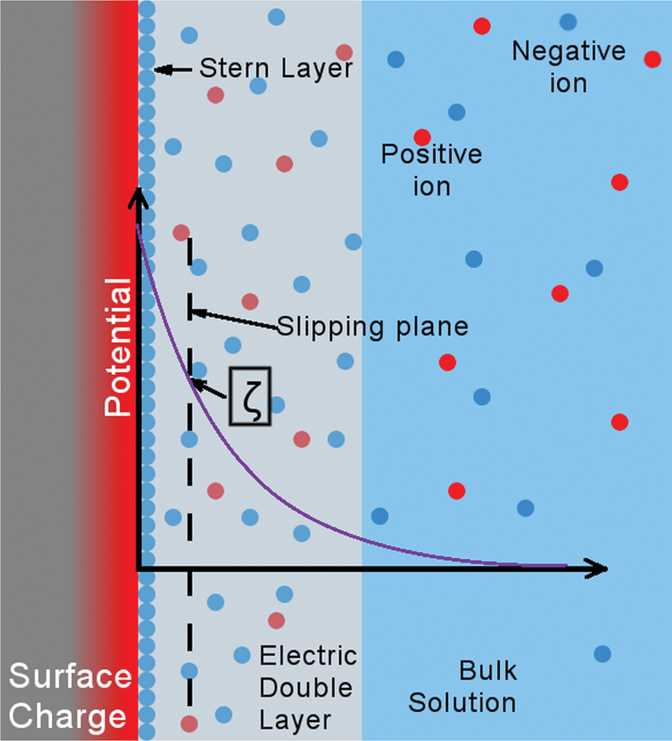
Diagram of charge distribution and electrical potential at a surface-solution interface. The Stern layer is filled with immobile ions with opposite charge of the surface. The slipping plane is the position away from the surface where particles can move due to applied shear stress rather than just diffusion. The zeta potential is the electrical potential at the slipping plane relative to the bulk solution.

Direct measurement of the zeta potential on the inside of a nanoscale channel is not currently technically possible, but it can be calculated from other measurements, specifically the streaming potential. The streaming potential is a voltage that arises along the length of a channel (E_z) from the movement of ions due to pressure-driven liquid flow and the interaction of those ions within the EDL. The streaming potential (dE_z/dΔP) is a function of the zeta potential following the Helmholtz-Smoluchowski equation. ¹

$$\left(\frac{d{E}_z}{d\Delta P}\right)=\frac{{\epsilon }_0{\epsilon }_r\zeta }{\eta {\Lambda }_0},$$

(3)

where Λ₀ is the solution conductivity.

After measuring the streaming potential, equations (1), (2), and (3) can be used to determine the surface charge density on the interior of a pore, allowing for greater insight into the design of charge-based filtration applications with that filter.

Although the streaming potential can be of great use in determining the zeta potential of a membrane, there are some limitations to this approach. Equation (3) can only be applied in situations where the EDL thickness is much smaller than the critical dimension of the pore itself, such that the vast majority of the solution in the pore is bulk solution. In addition, determining the Debye length for solutions with more than two types of ions or asymmetric ion content has not yet been solved. ⁶

Materials and Methods

Experimental Apparatus

The experimental apparatus developed in this study uses a modular approach. Individual components include the test fixture, voltage-controlled pressure regulators (VCPR), data acquisition pod (DAQ pod), digital multimeter (DMM), liquid reservoirs, and a computer for instrument control and data acquisition. The test fixture was custom built and is described below. All other physical components are commercially available.

Test Fixture

A custom-designed streaming potential ultrafiltration cell (SPUC; Fig. 2 ) was fabricated using stereolithographic rapid prototyping. There are two sections to the SPUC, labeled as the primary and secondary sections. Each section has inlet and outlet ports that run from a 10–32 threaded fitting to a rectangular duct that leads to the filtration chamber, which is bounded by the membrane and the SPUC section. The rectangular ducts and filtration chamber are designed to provide uniform shear and mass transfer across the membrane area during cross-flow filtration experiments, for which SPUC was also designed. Ports for monitoring side pressures are incorporated into each section. A replaceable silver wire is embedded into each SPUC section, recessed into the bulk of the section so that the electrode will not come into contact with the filter surface. The use of stereolithographic rapid prototyping for the ultrafiltration cell in combination with the modularity of the testing system as a whole greatly increases the flexibility of filters, which can be characterized by streaming potential measurements.

Figure 2.

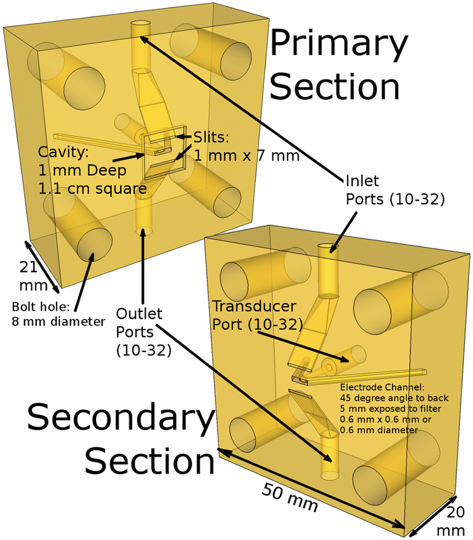
Diagram of fabricated streaming potential test mount (streaming potential ultrafiltration cell [SPUC]) sections. Each section has an inlet and outlet port for liquid flow past the filter. There is also a transverse port for measuring the pressure on each side of the filter. Electrode channels fix the position of the Ag/AgCl electrode used for measuring transmembrane voltages. The primary section has a shallow cavity (1 × 1 cm) for holding the planar filter that is to be tested.

The filter to be tested is secured in the square recess of the primary section. A square PDMS gasket separates the filter from the primary section. The interior walls of the gasket, along with the chip and the face of the recess in the primary section, create the filtration chamber for the primary section. A larger 5 × 5-cm PDMS backplane, with a square cutout in the middle to form the filtration chamber for the secondary section, is aligned with the primary section. The secondary section is then fitted to the other assembled parts. The entire assembly is secured together with four bolts that pass through the holes in the corners. This method of securing the filter forms an air-tight and liquid-tight seal without modifying or bonding the filter, allowing for the possibility of measuring the streaming potential of an individual filter before and after chemical treatment.

Before streaming potential testing is performed, the system is filled and flushed with deionized (DI) water to remove any stray ions within the filter. The interior of the filter is flushed with DI water using a volume of at least 50 L/m² of pore area. The system is then flushed with the testing solution using a volume of at least 50 L/m² of pore area prior to measuring the streaming potential.

System Assembly

When the filter has completed pretest preparations, the streaming potential measurement system is set up as shown in Figure 3 . As described above, the SPUC secures the filter in place between a PDMS gasket and a PDMS backplane. Two air-tight liquid reservoirs containing the testing solution are connected via tubing to the SPUC. The two liquid reservoirs are pressurized by the VCPRs (IP413-020; Omega, Stamford, CT), which are controlled through a data acquisition and control (DAQ) pod (NI USB-6008; National Instruments, Austin, TX). The two VCPRs are set up to take a 0- to 10-V input voltage. In this configuration, a 1-V input to the VCPR results in 11 kPa of applied pressure.

Figure 3.

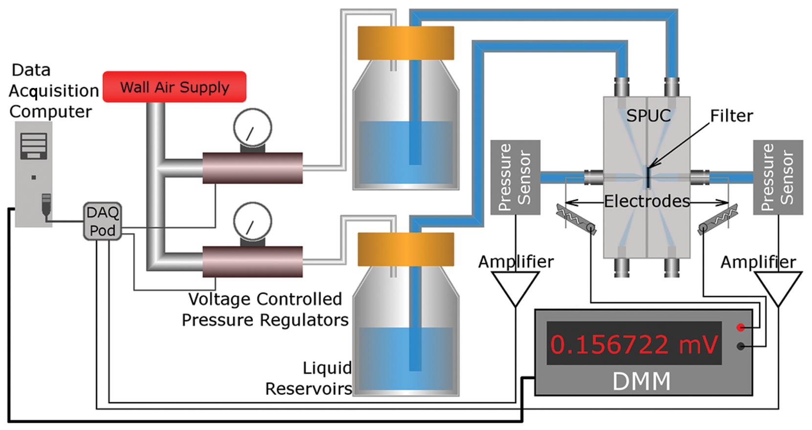
Diagram of the automated streaming potential measurement system. The data acquisition computer manages the data acquisition (DAQ) pod, which provides the input signal for the voltage-controlled pressure regulators (VCPRs). The VCPRs apply pressure to one of two liquid reservoirs using a wall air supply for high-pressure air. The applied pressure is read by a disposable pressure transducer and fed back to the DAQ pod after amplification of the signal. The feedback pressure reading is used in a PID controller to ensure that the applied pressure is the same as the set pressure. The voltage difference between Ag/AgCl electrodes placed in the primary and secondary sections is measured by a digital multimeter (DMM), which is periodically queried by the computer.

The pressure on each side of the test mount is measured by a pressure transducer (DTXPlus; BD, Franklin Lakes, NJ). The signals from the pressure transducers are individually amplified by differential amplifier circuits built in-house ( Fig. 4 ). The amplified signals are then read by the DAQ pod. The combination of pressure transducer, amplifier, and the analog-to-digital conversion in the DAQ pod provides pressure measurements with a precision of 40 Pa.

Figure 4.

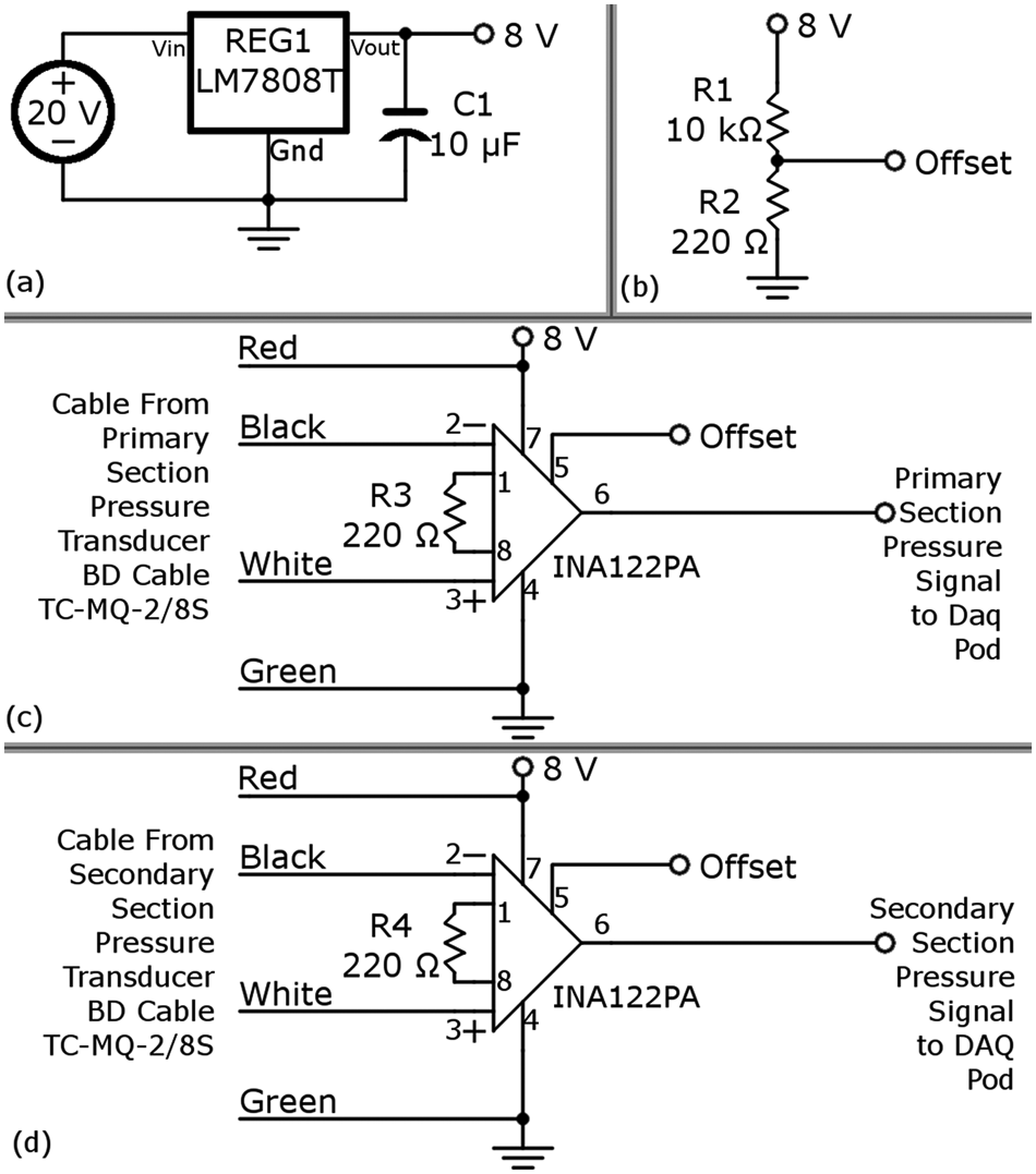
Schematic diagram for control circuitry. (a) Depicts a regulator which provides 8 V to the rest of the circuit. Part (b) provides an offset to the amplifiers so that a zero-pressure measurement will have a nonzero voltage associated with it. Parts (c) and (d) are the amplifiers that connect to the pressure transducers on the primary and secondary sections, respectively. The outputs of these amplifiers are measured using the data acquisition (DAQ) pod. DMM, digital multimeter; SPUC, streaming potential ultrafiltration cell.

The voltage across the filter is measured using two Ag/AgCl electrodes connected to a DMM (Keithley 2000; Keithley Instruments, Cleveland, OH) with 0.1 µV resolution. The Ag/AgCl electrodes area is created by driving a 5-mA current through 0.5-mm-diameter silver wire for 20 min while immersed in 1 M potassium chloride (KCl), using the silver wire as an anode. ¹ Both the DMM and the data acquisition pod are connected to and controlled by a dedicated computer.

PID Controller

A proportional-integral-derivative (PID) controller is a class of feedback-based controller. In a system where the error is defined as the difference between the set point and the output, a PID controller provides compensation based on the value of the error itself, the accumulated error over time, and the rate of change of the error. A digital implementation of a PID controller was custom written to ensure that the applied pressure across the membrane is brought to and maintained at the desired pressure. A standard implementation of an analog control system with a PID controller is shown in Figure 5 . The standard transfer function for an analog PID controller in the s-domain from the Laplace transform is the following ⁷ :

$$D(s)=\frac{U(s)}{E(s)}=K\left(1+\frac{1}{T_{\mathrm{I}}\cdot s}+T_D\cdot s\right),$$

(4)

where K is the overall gain, T_I is the integral time constant, and T_D is the derivative time constant. The signal U(s) is what is sent to the VCPR, and the error signal E(s) is the difference between the set pressure (R(s)) and the measured transmembrane pressure (Y(s)). The variable s can be treated as a derivative in the time domain, and 1/s can be treated as a time domain integral. Multiplying equation (4) by s·E(s) results in an equation with no denominator containing s or a function of s, removing time domain integrals from the equation:

$$s\cdot U(s)=K\left(T_D\cdot s^2\cdot E(s)+s\cdot E(s)+\frac{E(s)}{T_{\mathrm{I}}}\right).$$

(5)

Figure 5.

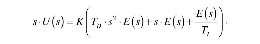
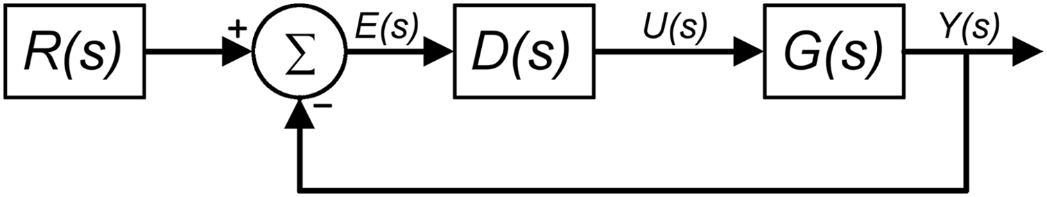
Block diagram for analog control system. R(s) is the set pressure. E(s) is the error between the set pressure and the measured pressure; D(s) is the compensation, which is a proportional-integral-derivative (PID) controller in this case; and G(s) is the transfer function for the uncompensated system.

The corresponding time signals for U(s) and E(s) are u(t) and e(t). Dropping the (t) and using the dot notation for derivatives (i.e., ë is the second time derivative of e),

$$\dot{u}=K\left(T_D\cdot \ddot{e}+\dot{e}+\frac{e}{T_I}\right).$$

(6)

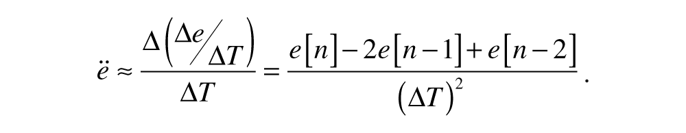
When the signals are digitized, they are represented by discrete values separated in time by the sampling period ΔT (which is set by the user in the custom software). The discrete signals become u(nΔT) and e(nΔT). For a sequence of values u[0], u[1], u[2] . . . corresponding to the time signal u(0), u(ΔT), u(2ΔT). . ., an estimate of the derivative of the analog signal between any two consecutive points can be calculated as

$$\dot{u}\approx \frac{\Delta u}{\Delta T}=\frac{u\left[n\right]-\left[n-1\right]}{\Delta T}.$$

(7)

The same situation can be applied to the equations for e as well. For an estimate of the second derivative of e, simply perform the same operation again, which yields the following result:

$$\ddot{e}\approx \frac{\Delta \left(\raisebox{1ex}{$\Delta e$}\!\left/ \!\raisebox{-1ex}{$\Delta T$}\right.\right)}{\Delta T}=\frac{e\left[n\right]-2e\left[n-1\right]+e\left[n-2\right]}{{\left(\Delta T\right)}^2}.$$

(8)

Recognizing that u[n + 1] and u[n] can also be used for estimating the time derivative for u, a value for u[n + 1] can be obtained from u[n], e[n], e[n − 1], and e[n − 2] by combining equations (6), (7), and (8) and solving for u[n + 1]:

$$u\left[n+1\right]=K\left(e\left[n-2\right]\frac{T_D}{\Delta T}-e\left[n-1\right]\left(\frac{2T_D}{\Delta T}+1\right)+e\left[n\right]\left(\frac{T_D}{\Delta T}+1+\frac{\Delta T}{T_I}\right)\right)+u\left[n\right].$$

(9)

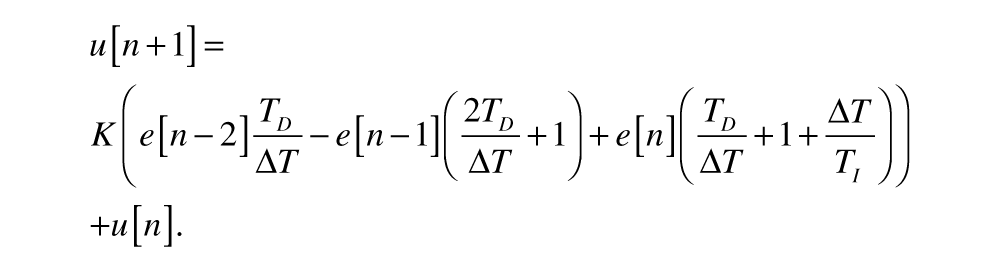
The units for u, e, y, and r are stored internally as values denominated in Pa. The transition from the measured voltage from the pressure transducers to Pa is performed using the calibration of the sensors done during the initialization phase. As mentioned earlier, the VCPR applies 11 kPa of pressure per volt of input. As such, the internally stored number for u[n + 1], if positive, is divided by 11 000 and the resulting value, in volts, is applied to the VCPR for the primary section via the DAQ pod, and the input to the VCPR to the secondary section is set to 0. For negative values of u[n + 1], the magnitude of u[n + 1]/11 000 is applied to the VCPR for the secondary section, and the primary section VCPR is set to 0.

Computer Control

Custom software was written using Microsoft Visual C# Express 2008 to collect data from the DMM and data acquisition pod as well as to control the values on the analog outputs of the data acquisition pod. Figure 6 illustrates the various steps performed by the software in the course of measuring the streaming potential of a filter. The first five steps in Figure 5 represent tasks that require user input, including calibration of the pressure transducers, and setting the pressures, number of cycles, controller coefficients, and sampling period. When these initialization tasks have been finished, data acquisition may begin.

Figure 6.

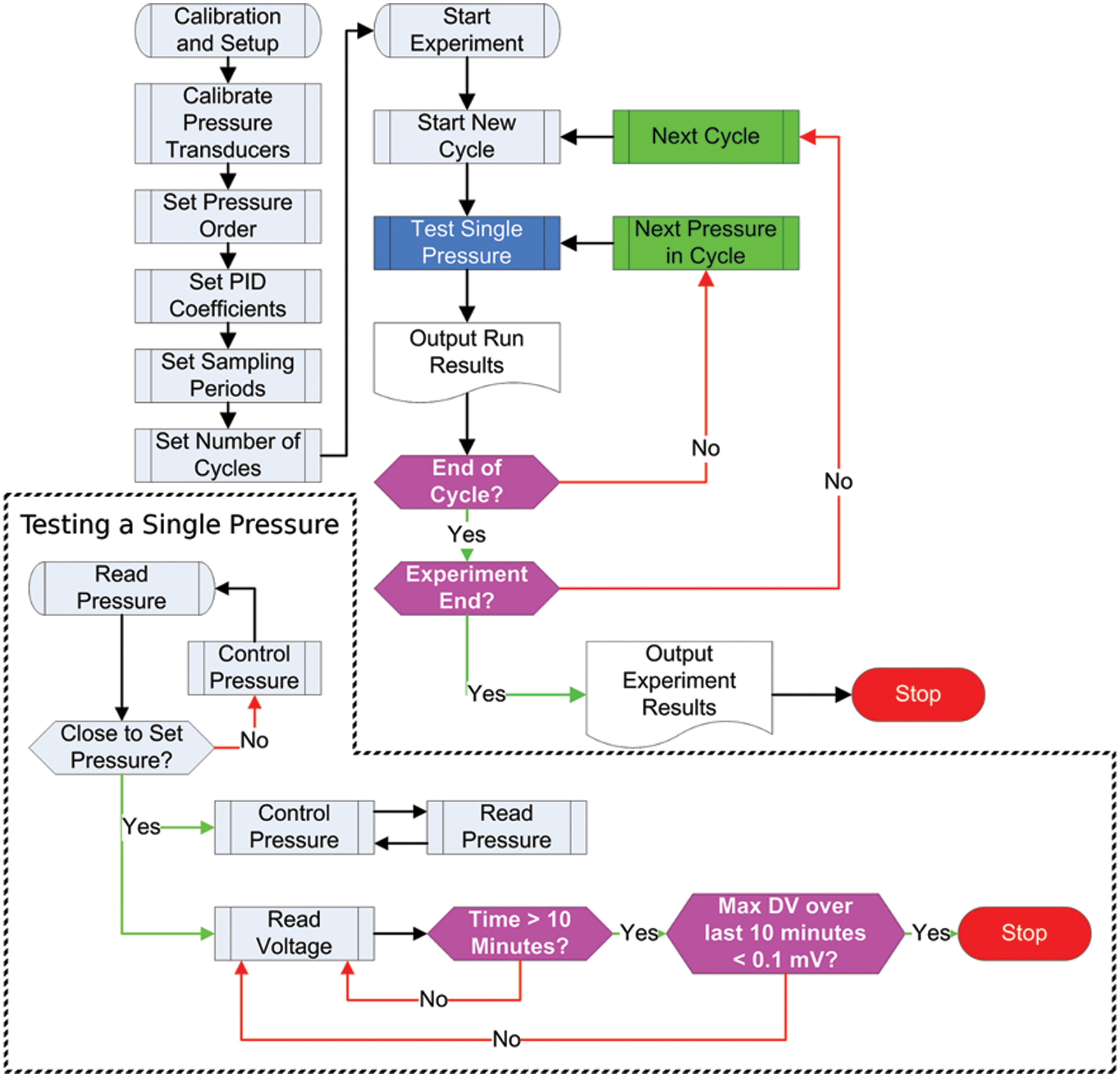
Flowchart describing the control sequence for an experiment performed by the custom written software. The first five steps require inputs from the user. Once data acquisition has been started, the user does not need to interact with the system. The tasks that the software goes through during the “Testing a single pressure” step are shown in the dashed box on the bottom.

Once data acquisition has started, the software cycles through the pressures set by the user. During a cycle, the program sequentially measures the transmembrane voltage for each input pressure. The dashed box at the bottom of Figure 6 outlines the sequence during the testing of a given input pressure or set pressure. Testing at a single pressure is referred to as a run. First, the transmembrane pressure is measured and compared with the set pressure. The PID controller described previously drives the VCPRs based on the error between the measured and set pressures. PID coefficients representing an overdamped system, which achieves the set pressure to within 300 Pa in approximately 30 to 45 s, are loaded when the control software is started. The overdamping of the system is deliberate so pressure transients that could damage the filter are minimized. These coefficients can be changed by the user.

When the measured pressure is within 300 Pa of the set pressure, voltage readings commence. The applied pressure continues to be managed by the PID controller. The transmembrane voltage is considered to be stabilized when the difference between the maximum and minimum voltages for the previous 10 min is <0.1 mV. Once the transmembrane voltage has stabilized, the run is completed and the results are saved in a comma separated value (CSV) file. If the just finished run was the last run in a cycle, a new cycle begins immediately. If the just finished run was the last run in the experiment, a CSV file containing a summary of all of the runs is saved, and the transmembrane pressure is slowly released by setting the set pressure to 0 Pa and allowing the PID controller to reduce the pressure. When the transmembrane pressure is between −300 Pa and 300 Pa, the inputs to both VCPRs are set to 0, allowing the rest of the pressure to be released.

System Calibration

Pressure Measurement

At the start of an experiment, the pressure measurement system is calibrated by applying at least three separate pressures to each DTXPlus by means of a hydrostatic water column and measuring the resulting voltage from the associated amplifier. Linear regressions of voltage versus water column pressure for both pressure transducers are calculated and used as the calibration curves for the experiment. A new calibration is performed prior to any subsequent experiment.

PID Controller

To calibrate the pressure system, a handheld pressure readout device designed to work with the DTXPlus pressure transducers was used. The readout also contained an analog out, which was the directly amplified signal from the DTXPlus. The voltage from the analog out was measured using a Tektronics TDS 420A digital oscilloscope (Tektronics, Beaverton, OR). A VCPR was set up to provide pressure to a liquid reservoir filled with DI water, which was connected to a length of tubing terminated with a DTXPlus. The oscilloscope was put into trigger mode, and a step function of 1 V was applied to the input of the VCPR.

The steady-state reading of the handheld pressure readout after applying the step function was 11 kPa. The voltage response of the analog output of the pressure readout and the corresponding pressure is shown in Figure 7 . The decaying exponential model shown with the actual response has the following function:

$$\text{Model}=11.000\left(1-e^{-11.513t}\right)\left[\text{kPa}\right].$$

(10)

Figure 7.

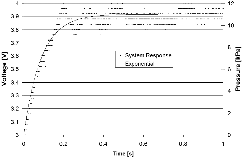
Response of voltage-controlled regulator and pressure transducer to a 1-V step input applied to the system. A decaying exponential equal to 11.000(1 − e^−11.513t) [kPa] is shown along with the voltage output of the DTXPlus amplified by the handheld pressure readout.

By treating all of the data points from 0 to 1.5 s as vectors for both the response and the model, the inner product divided by the respective magnitudes of the two vectors yields a value of 0.999. For a perfect match, this product would be 1 exactly. Using equation (10) and the fact that the response was the result of a step response, an analog transfer function for the system can be determined to be

$$G(s)=11.000\left(\frac{11.513}{s+11.513}\right).$$

(11)

Equations (4) and (11) can then be used in conjunction with the system model shown in Figure 5 to determine the desired values for T_I, T_D, and K. The default values that are preset into the software (but can be changed by the user) are K = 0.003, T_I = 0.025, and T_D = 0. These parameters yield a system settling time of 30 to 45 s.

Results

System Characterization

The CSV files that were created after each run provide the elapsed time from the start of the run, the measured pressures, and the transmembrane voltage at each instance that the voltage was measured. Analysis of these files can provide insight as to the characterization of the system.

Table 1 shows the minimum, maximum, and average values for some characteristics of the system compiled from 90 individual runs. The lead time is the time between when a run starts and when the set pressure is achieved to within 300 Pa. $\left|\overline{P}-P_{set}\right|$ is the magnitude of the error between the average pressure measured over the last 10 min of the run and the set pressure. Max V − Min V is the maximum voltage differnece between any two data points during the last 10 min of the run. The values reported for the lead time in Table 1 are similar to those desired from the previous section, although the minimum and maximum values measured are both outside of the 30- to 45-s settling time desired but by less than 5 s in each case.

Table 1.

Characteristics of the System Based on 90 Individual Runs

	Minimum	Maximum	Mean
Lead time, s	25.4	46.1	35.8
$\left|\overline{P}-P_{set}\right|$ , Pa	3	120	37
Max V − Min V, mV	0.010	0.078	0.025

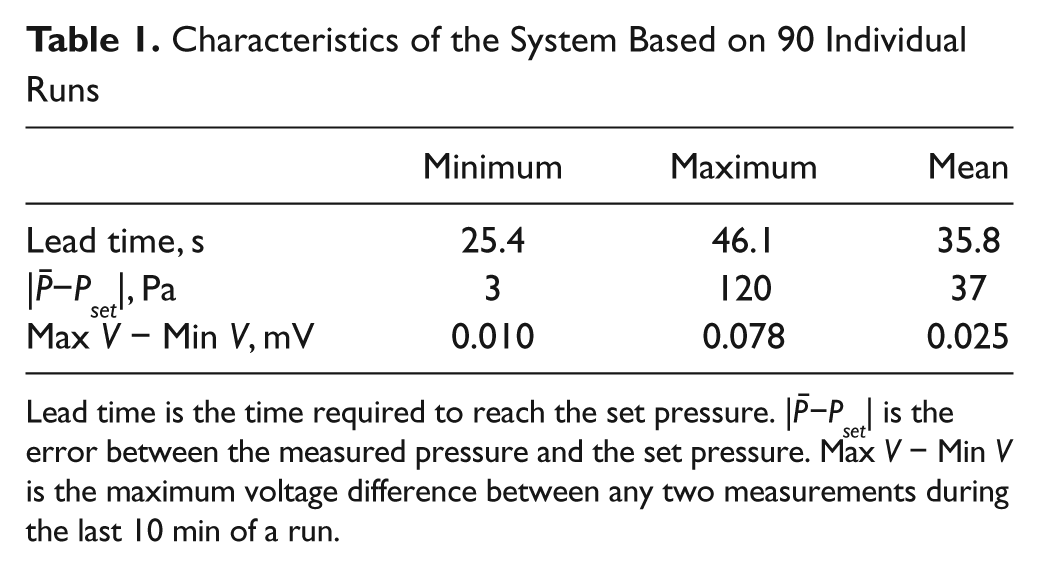
Lead time is the time required to reach the set pressure. $\left|\overline{P}-P_{set}\right|$ is the error between the measured pressure and the set pressure. Max V − Min V is the maximum voltage difference between any two measurements during the last 10 min of a run.

The PID controller does well at maintaining the pressure, with an average error less than 50 Pa and a maximum error of only 120 Pa. The results for the maximum voltage difference indicate that even with the maximum allowed voltage difference of 0.1 mV, most runs do not come near this value, with a maximum voltage difference of 0.078 mV and a mean difference of 0.025 mV.

Experimental Use

The filter employed for testing the streaming potential measurement system is the Biomax 100 (Millipore, Bedford, MA), which is a commercially available polyethersulfone (PES) membrane. This zeta potential of the Biomax 100 membrane has been well characterized by Burns et al. ¹ in an array of testing solutions. In contrast to the method described herein, the method used by Burns et al. involved applying a transmembrane pressure by physically raising or lowering a liquid reservoir to generate different hydrostatic pressures or by applying pressurized air to a liquid reservoir. In addition, only positive pressures, up to 35 kPa, were applied. Their system was allowed to stabilize at a given pressure for 30 min, at which time the transmembrane voltage was recorded, ¹ whereas our system recorded an average transmembrane voltage for a 10-min period after the voltage was determined to have stabilized.

The testing solution used for the current experiment was 10 mM KCl buffered with 1 mM Tris, prepared by dissolving preweighed amounts of KCl and Tris into a known volume of DI water and then adjusting to a pH of 7.0 using small aliquots of 1 M HCl or 1 M KOH. The solution conductivity was 1.41 mS/cm. The applied pressures for one cycle were, in order, 3 kPa, 15 kPa, 9 kPa, −3 kPa, −15 kPa, and −9 kPa. This cycle was repeated 15 times.

The measured transmembrane voltages for each cycle are shown graphically in Figure 8 . Each cycle was extremely linear with the lowest coefficient of determination greater than 0.9995. The average measured streaming potential was 59.5 ± 0.5 µV/kPa. This corresponds to a zeta potential of −11.8 ± 0.1 mV for a conductivity of 1.41 mS/cm. The average result reported by Burns et al. ¹ for a Biomax 100 in the same solution was −12.9 ± 0.6 mV. However, it was mentioned in that study that streaming potentials, and thus zeta potentials, of different specimens could vary by up to 20%. As such, our results are consistent with the previously published data when such variability is taken into account.

Figure 8.

Individual pressure cycles measured using the automated streaming potential testing system. As can be seen, each cycle is linear. The lowest R² for any individual cycle was greater than 0.9995. The average measured streaming potential was 59.5 ± 0.5 µV/kPa. For a conductivity of 1.41 mS/cm, this corresponds to an apparent zeta potential of −11.8 ± 0.1 mV.

Discussion

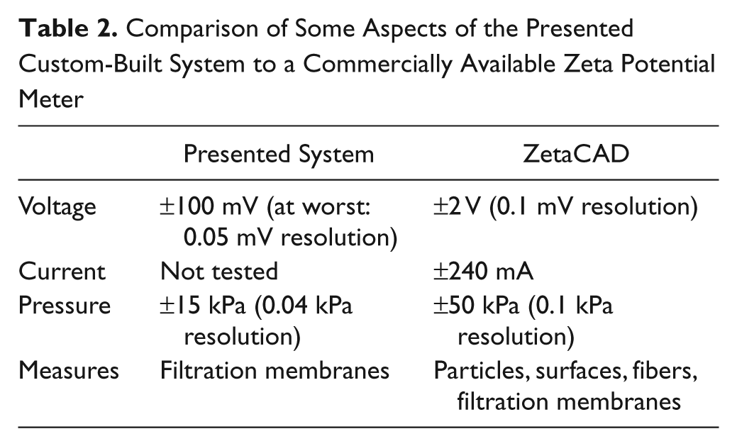
The idea of an automated zeta potential meter is not new, and some are commercially available. Table 2 provides a quick comparison of the streaming potential performance of the presented custom system to that of a commercially available system. The voltage range reported for the custom system is the range in which the resolution of the Kiethley 2000 Multimeter is 0.1 µV. The custom system has not been tested outside of this range. As can be seen in Table 2 , the two systems are largely comparable when measuring the streaming potential of a filter, with the commercial system having a larger voltage range, larger pressure range, but lower pressure resolution. For the processes of interest to the authors, the pressure and voltage ranges provided by the custom system are sufficient. Should other researchers require a greater pressure range, a different VCPR and pressure transducer could replace the Omega IP413-020 and the BD DTXPlus. A new amplifier circuit may also have to be designed to provide the proper gain from a different pressure transducer. These separate parts, however, would do little to increase the overall cost of the system.

Table 2.

Comparison of Some Aspects of the Presented Custom-Built System to a Commercially Available Zeta Potential Meter

	Presented System	ZetaCAD
Voltage	±100 mV (at worst: 0.05 mV resolution)	±2 V (0.1 mV resolution)
Current	Not tested	±240 mA
Pressure	±15 kPa (0.04 kPa resolution)	±50 kPa (0.1 kPa resolution)
Measures	Filtration membranes	Particles, surfaces, fibers, filtration membranes

In practical terms, knowing the zeta potential of a filter allows for better design of filtration processes if the electrostatic properties of the filter itself can be harnessed. An understanding of the filter’s zeta potential could also lead to prediction of any effects that are influenced by the electrical potential at the liquid–solid interface. The system presented in this work allows for the rapid determination of a planar filter’s streaming potential while removing the tediousness of manually controlling the pressure and recording voltages. For the SPUC used in this work, any 1 × 1-cm planar filter can be readily tested. For different filter designs, a new ultrafiltration cell can be created quickly by stereolithic rapid prototyping.

We have developed a low-cost automated system for measuring the streaming potential of arbitrary filters. Although the ultrafiltration cell was designed specifically for 1 × 1-cm planar filters, the modular approach to the measurement and the method used to fabricate the ultrafiltration cell allow for other filter shapes or styles to be incorporated with little, if any, modification to the rest of the system and at low cost.

The system was tested using a Biomax 100 membrane with 10 mM KCl buffered to a pH of 7 with 1 mM of Tris. The streaming potential for this combination had been previously reported in the literature, ¹ and results from the automated testing system were in agreement with those previously reported.

This system provides a substantial benefit at a relatively low cost (<$4000). The capacity to measure the streaming potential without the oversight of an operator after initialization allows the researcher to characterize the charge-based effects of a particular filter with fewer man hours as well as reducing the overall length of time needed for the characterization. Finally, the automation of the characterization process minimizes the effect of operator influence on the outcome of the experiment.