
Abstract
This study investigates the causal impact of Rural Non-Farm Employment (RNFE) on household income and consumption in rural Uttar Pradesh (UP), India, a region facing persistent poverty and agrarian distress. The objective is to assess whether engagement in non-farm economic activities significantly enhances rural welfare outcomes, thereby providing an effective avenue for poverty alleviation. The novelty of this research lies in its state-specific focus on UP, a region often neglected in national studies, and its application of a counterfactual framework to rigorously estimate causal effects using observational data. This study utilizes unit-level data from the Periodic Labour Force Survey (PLFS) 2019–20. To mitigate concerns related to selection bias and endogeneity, the analysis employs the Propensity Score Matching (PSM) technique, incorporating both Nearest Neighbour Matching (NNM) and Kernel-Based Matching (KBM) approaches. The results show that RNFE participation raises monthly per capita income by ₹412 (NNM) and ₹416.8 (KBM), and increases monthly per capita consumption expenditure by ₹97, compared to agricultural workers. These effects place RNFE participants significantly above the poverty line, reinforcing the role of RNFE in poverty alleviation. Importantly, the study finds that regional disparities persist within UP, with Western UP benefiting more due to possibly better-quality non-farm jobs. The findings underscore the need for region-specific employment strategies that improve the quality, accessibility, and inclusiveness of RNFE. By offering robust empirical evidence, this research contributes to the broader discourse on rural transformation and supports more effective, evidence-based rural development policy in India.
Plain Language Summary
This study examines the impact of Rural Non-Farm Employment (RNFE) on household income and consumption in rural Uttar Pradesh, India, focusing on poverty alleviation. Using a counterfactual framework, the study employs Propensity Score Matching to estimate causal effects from the Periodic Labour Force Survey 2019-20. Results show RNFE significantly increases monthly per capita income and consumption, elevating participants above the poverty line. Regional disparities exist, with Western UP benefiting more due to better non-farm jobs, emphasizing the need for region-specific employment strategies. The study supports RNFE's role in rural transformation and urges policies enhancing employment quality and inclusiveness. This research examines RNFE's impact on alleviating poverty and improving household income in rural Uttar Pradesh, a region affected by poverty and agrarian distress. By focusing on RNFE as a tool for poverty alleviation, the study provides insights into how livelihood diversification contributes to economic resilience. The research uses rigorous methodologies to establish causal relationships, offering evidence-based recommendations for policy-making. Key Takeaways: 1. Economic Impact: RNFE participation significantly increases household income and consumption, suggesting non-farm employment can improve rural economic outcomes and lift households above poverty. 2. Regional Disparities: The study reveals regional inequalities within Uttar Pradesh, with Western UP benefiting more from RNFE due to higher quality non-farm jobs, indicating the need for tailored strategies. 3. Policy Implications: The research emphasizes developing region-specific policies to enhance RNFE quality, accessibility, and inclusiveness for poverty reduction and rural development.
Introduction and Background
Poverty alleviation and rural development remain persistent challenges in India, particularly in populous and agrarian states such as Uttar Pradesh. Despite several policy interventions, a substantial portion of the rural population continues to experience underemployment, low productivity, and income vulnerability due to an overdependence on agriculture (Chand et al., 2014). Given the seasonal and increasingly uncertain nature of agricultural incomes, diversification through Rural Non-Farm Employment (RNFE) has emerged as a critical strategy for enhancing livelihood security, promoting rural resilience, and achieving inclusive growth (Himanshu et al., 2016). Evidence from Sub-Saharan Africa and South Asia shown that, rural households increasingly diversify their incomes through non-farm activities that not only provide alternative income sources but also improve food security, resilience to economic shocks, and overall household well-being (Ba et al., 2021; Tesfaye & Nayak, 2022).
Over the last two decades, rural India has witnessed substantial expansion in the non-farm sector, which includes a diverse range of activities such as manufacturing, trade, construction, and services (Goel, 2024). In states such as Uttar Pradesh, where challenges such as land fragmentation, inadequate irrigation, limited public investment in agriculture, and low agricultural productivity constrain the potential for farm-based economic growth, the rural non-farm economy assumes a particularly crucial role in sustaining rural employment and livelihoods (Fan et al., 2008; Lanjouw & Murgai, 2009; Chand et al., 2011; Singh, 2012; Hashmi, 2024). Moreover, the RNFE sector often absorbs surplus labour from agriculture and creates employment opportunities for women and marginalized groups, thereby fostering socio-economic inclusion (Start, 2001). Many researchers consider rural non-farm activities as a strategy for mitigating rural poverty and addressing rural–urban disparities (Abdul-Hakim & Hadijah, 2011; Foster & Rosenzweig, 2004).
Uttar Pradesh, amongst India's most populous states, serves as an apt case study due to its heavy reliance on agriculture and varied agrarian development. Uttar Pradesh has been one of the worst-performing states on many counts, with 29.4% of its population below the poverty line in 2011-12, which is almost 9 % points higher than the national average. Moreover, the proportion of people living in poverty in rural areas of UP was calculated to be 33.4%, which is considerably above the 25.7% national average for rural regions (Government of Uttar Pradesh, 2016-17). The state has witnessed a steady and persistent rise in rural non-farm employment, highlighting its increasing significance in rural livelihoods and income generation (Hashmi, 2025; Himanshu et al., 2016; Mishra & Singh, 2018; Ranjan, 2009). Despite the growing importance of rural non-farm activities, the extent to which they influence rural consumption and income remains unexplored in the state. Enhancements in income and consumption through engagement in RNFE are crucial for states like Uttar Pradesh, as they contribute to poverty alleviation and reflect the overall well-being of rural households. This underscores the significance of the present study, which seeks to evaluate the impact of RNFE on income and consumption. Most existing studies on RNFE either adopt a pan-India approach or focus on southern or western Indian states, where the non-farm sector is relatively more developed and formalized (Himanshu et al., 2011; Kaur, 2019). Very few studies isolate the state-specific dynamics of UP, where structural constraints, poor infrastructure, and gender disparities pose unique challenges to the expansion and inclusiveness of RNFE (Kapoor et al., 2021; World Bank, 2011).
Moreover, many existing analyses face challenges related to endogeneity and selection bias, since the choice to participate in non-farm employment is shaped by a range of household traits, some of which may not be directly observable. To mitigate this concern, the Propensity Score Matching (PSM) technique provides a rigorous framework for estimating the causal impact of RNFE. By creating a counterfactual scenario, it enables the comparison of individuals engaged in non-farm work with those who are not, but who share similar observable characteristics (see Jalan & Ravallion, 2003; Rosenbaum & Rubin, 1983).
This study seeks to fill a crucial gap in the literature by rigorously examining the impact of RNFE on household consumption and income in rural Uttar Pradesh using nationally representative microdata and PSM methodology. The findings aim to contribute to the academic discourse on rural transformation and offer evidence-based insights for policymakers designing employment and poverty alleviation strategies in lagging rural economies.
Theoretical Framework and Literature Review
The Lewis Dual Sector Model (Lewis, 1954) serves as the fundamental theoretical basis for reducing poverty through non-farm employment. As the non-agricultural sector grows, it absorbs excess labour from agriculture, boosts labour productivity, and results in increased household incomes and consumption. This shift is viewed as a means of achieving structural transformation and reducing poverty. Rural households often experience significant income fluctuations due to agriculture’s reliance on weather conditions. Ellis (2000) highlights that diversifying livelihood, including participation in non-farm work, mitigates income risk and stabilizes consumption. The Household Economic Portfolio Model considers rural households as multi-activity economic entities that distribute labour and capital across various livelihood options to maximize utility. Non-farm employment is part of a household’s strategy to optimize resource utilization, stabilize income, and break free from poverty, especially when landholdings are limited or unproductive (Barrett et al., 2001). Haggblade et al. (2010) contend that the non-farm sector significantly contributes to rural development not only through direct employment but also via multiplier effects. Income generated from the rural non-farm employment enhances demand for local goods and services, stimulates the development of local enterprises, and facilitates rural market integration. These forward and backward linkages foster a more dynamic rural economy, thereby alleviating poverty for both participants and non-participants.
A substantial body of research has highlighted the essential role of the rural non-farm sector in creating employment opportunities and alleviating poverty. For example, Ravallion and Datt (1996) emphasize that the expansion of non-agricultural activities in rural regions has positively influenced poverty reduction, particularly for smallholders and land-constrained households. Hazell and Haggblade (1991) similarly note that such sectors contribute to the development of rural human capital and skill formation. Lanjouw and Shariff (2004) highlight the role of shifting agricultural wage dynamics and the extent of agricultural employment in shaping rural poverty outcomes. Despite these insights, there remains limited empirical clarity on whether diversification into RNFE consistently leads to poverty reduction. In a detailed village-level case study of Palanpur, Himanshu et al. (2013) observed that participation in the non-farm sector not only boosted household incomes and reduced poverty levels but also helped break long-standing social mobility constraints affecting marginalized rural groups. Supporting these findings, Imai et al. (2015), through comparative analysis of Vietnam and India, found that non-farm employment, particularly in skilled roles, had a notable impact in lowering poverty and economic vulnerability. They argue that households engaged in diverse, non-agricultural livelihoods were more resilient to financial shocks. Pattayat et al. (2022) also contend that access to non-farm employment reduces the likelihood of rural poverty. Likewise, a recent study by Baysan et al. (2024) using real-time data from casual laborers in Jharkhand documented that a shift from agricultural to non-agricultural work resulted in an average wage gain of approximately 23%. This wage differential further underscores the economic incentive for rural workers to transition into non-farm employment.
In several developing nations, the expansion of rural non-farm activities is increasingly viewed as a vital approach to combating poverty. Asiimwe et al. (2025), through the application of propensity score matching techniques, reported that involvement in non-farm sectors leads to a marked decline in rural poverty, while simultaneously improving household consumption and upward income mobility. In a similar vein, Adeyonu et al. (2024), analyzing data from Nigeria, found that rural households engaged in non-farm occupations experienced a significantly lower incidence of poverty. Evidence from Bangladesh further supports this pattern. The poverty rate among rural households with access to non-farm income was found to be 15.4% compared to 22.7% among those without at the lower poverty line, and 27.1% versus 37.6% at the upper poverty line. These disparities underline the positive role of non-farm earnings in alleviating poverty. Supporting this, Hossain et al. (2018) employed the Foster, Greer, and Thorbecke (FGT) indices and demonstrated that non-farm income reduces not only the prevalence of poverty but also its depth and severity, both regionally and nationally across rural Bangladesh.
In Uganda, Watema et al. (2025) observed that household well-being, proxied by consumption expenditure and poverty status, improves significantly with greater non-farm income. Their analysis, based on an instrumental variable framework with robust standard errors, found that a 1% rise in non-farm income leads to a 20.9% increase in consumption expenditure and reduces the likelihood of a household being poor by approximately 59.5%. Similarly, Chekol (2024) highlighted the importance of creating enabling environments for women's participation in non-farm work in Ethiopia. The study noted that factors such as youth, livestock ownership, food insecurity, and market proximity significantly influence women’s likelihood of engaging in non-farm employment, which in turn plays a substantial role in reducing poverty. In Vietnam, Duong et al. (2021), using a difference-in-difference method coupled with kernel propensity score matching on two-period panel data, demonstrated that participation in off-farm employment contributes meaningfully to household welfare. Their findings indicate not only an increase in total household income but also improvements in food security and dietary diversity, along with reductions in poverty incidence, poverty gap, and overall poverty intensity.
Despite the expanding corpus of literature underscoring the significance of Rural Non-Farm Employment (RNFE) in poverty alleviation, income enhancement, and consumption stabilization across various developing nations, including India, a critical knowledge gap persists in state-specific analyses, particularly concerning Uttar Pradesh (UP). The majority of empirical investigations have predominantly focused on national-level assessments (e.g. Lanjouw & Shariff, 2004; Ravallion & Datt, 1996) or on other regions and countries such as Vietnam (Duong et al., 2021), Bangladesh (Hossain et al., 2018), and sub-Saharan Africa (Asiimwe et al., 2025; Watema et al., 2025). While these studies consistently affirm the positive impact of RNFE on rural welfare, they frequently lack the granular regional focus necessary to inform state-specific policy frameworks. Uttar Pradesh, as India’s most populous state with the highest rural population (Census 2011), presents a unique socio-economic context characterized by small landholdings, high population density, agrarian distress, and persistent rural poverty (Agricultural statistics at a glance, 2022; Economics and Statistics Division,GoI). The agricultural sector in UP is marked by low productivity, income volatility, and structural inefficiencies, compelling households to diversify their livelihoods. However, there is limited empirical evidence on how this diversification, particularly into RNFE, affects household income and consumption patterns within the state.
Furthermore, although Himanshu et al. (2013) and Baysan et al. (2024) acknowledge regional variations in RNFE outcomes, Uttar Pradesh has seldom been the primary focus. Most studies utilize national-level datasets or concentrate on better-performing states such as Tamil Nadu, Maharashtra, or Gujarat, where non-farm sectors are more developed. The underrepresentation of Uttar Pradesh in these analyses is problematic, especially given its critical role in India’s overall poverty landscape. Moreover, while some studies (e.g. Imai et al., 2015; Pattayat et al., 2022) employ advanced econometric methods such as propensity score matching (PSM) or instrumental variable analysis to evaluate RNFE impacts, few have applied these methods specifically within the context of UP. This limitation constrains our understanding of the causal relationships between non-farm employment, income enhancement, and consumption smoothing in the state. This study seeks to identify the socio-economic characteristics that influence participation in rural non-farm employment in this region. Furthermore, the study examines the extent to which rural non-farm employment can be considered a substitute or complement to agricultural income within the rural economic portfolio. Our analytical approach involves comparing the income and consumption patterns of households that are similar in observable characteristics but differ solely in their engagement in agricultural or non-agricultural employment. To identify these observationally equivalent households, we employed Propensity Score Matching (PSM) techniques, which were originally developed by Rosenbaum and Rubin (1983).
This study enhances the existing body of knowledge by quantifying the causal effect of non-farm employment on income and per capita consumption. The findings indicate that rural households involved in non-farm activities exhibit higher income levels and increased consumption expenditure compared to those in agricultural pursuits. Furthermore, the study proposes that this enhanced income and consumption mobility within the non-farm sector could potentially aid in poverty alleviation efforts. The paper is structured as follows: Sections 1 and 2 cover the introduction, theoretical framework, and literature review. Section 3 details the data sources and the methodology utilized in the research. Section 4 offers a descriptive analysis of the data, examining poverty trends, regional disparities, and wage growth patterns. Section 5 presents the results, which include the probit model, regional heterogeneity, matching diagnostics, and sensitivity analysis. Section 6 discusses the findings. Finally, Section 7 includes conclusion and policy recommendations.
Data Sources and Methodology
This study utilizes rural employment data from five major NSS rounds—namely the 50th (1993–94), 55th (1999–2000), 61st (2004–05), 66th (2009–10), and the more recent Periodic Labour Force Survey (PLFS) for 2019–20. These rounds collectively offer a robust timespan for analyzing employment patterns and shifts in rural India. The NSS datasets are especially valuable as they contain extensive socioeconomic and demographic information at the household level, allowing for a nuanced examination of the key drivers behind rural non-farm employment. To analyze variables such as household composition, individual characteristics, employment status, and sectoral affiliation, this study relies on unit-level data drawn from the respective Employment and Unemployment Surveys and the PLFS. Employment information is interpreted based on the usual principal activity status and subsidiary status classifications, ensuring consistency over time. This approach aligns with the framework proposed by Hashmi (2025), who emphasized the significance of longitudinal datasets in understanding livelihood diversification trends in rural Uttar Pradesh.
Furthermore, employment income is documented from three categories: regular salary, casual/daily wages, and self-employment. Monthly income from regular employment is recorded for the previous month, whilst self-employment earnings are noted for the past 30 days. Casual wage income is reported for the preceding week. To calculate monthly casual wage earnings, weekly figures are multiplied by four. These three income sources are then aggregated to determine each individual's monthly labour income.
Moreover, income derived from agricultural and other seasonal work is challenging to measure on a monthly basis. Consequently, when recording incomes for agricultural workers, the PLFS does not capture the previous month's earnings (which could be nil despite the worker being employed). Instead, acknowledging that the output value must be distributed across the entire year, it is ‘distributed over the entire production process based on past experience’ (Instruction manual PLFS report, 2019-20). This means that incomes are averaged out, reflecting a typical month's earnings rather than necessarily the previous month's income. Despite meticulous efforts to measure the gross value of agricultural income on a monthly basis, incorporating past experiences, it remains essential to account for potential biases and errors. For example, seasonal fluctuations in agricultural activities can skew monthly estimates, while irregular and in-kind earnings are frequently underreported. Additionally, recall errors, the practice of joint family farming, and the omission of input costs further compromise accuracy. The survey may also overlook subsistence production and non-monetized exchanges. Collectively, these limitations contribute to the underestimation or misrepresentation of actual agricultural income.
In PLFS data, Rural Non-Farm Employment (RNFE) is defined as all income-generating economic activities excluding crop cultivation, animal husbandry, and fishery, undertaken by rural individuals. These activities include manufacturing, construction, trade, transport, and a variety of service sectors. However, the rural labour market is characterized by high levels of multiple job holding and seasonal shifts in employment, which necessitates a careful operationalization of employment categories.
To address this, the present study adopts the Usual Status approach as defined by PLFS, which accounts for the activity status over a reference period of 365 days. An individual is considered a participant in RNFE if they are engaged in any non-farm economic activity either in their usual principal activity (UPS) or in their usual subsidiary activity (USS). In accordance with the study's methodology, the treatment variable for participation in Rural Non-Farm Employment (RNFE) is defined as follows: RNFE is assigned a value of 1 if an individual is engaged in a non-farm activity (excluding agriculture, animal husbandry, and fishing) as either a principle or subsidiary occupation, as classified by the National Industrial Classification (NIC) or National Classification of Occupations (NCO). Conversely, RNFE is assigned a value of 0 if the individual is exclusively involved in agricultural activities in both principle and subsidiary status.
This approach allows the treatment variable to capture the complexity of rural livelihood patterns, including seasonal changes and diversified employment strategies. It ensures that the contribution of secondary employment in non-farm sectors is not overlooked, thereby providing a more comprehensive and accurate categorization of RNFE participation.
In addition, for the descriptive analysis, multiple rounds of NSSO data are employed to capture long-term trends in poverty, real wages, and the proportionate share of non-farm employment, thereby providing a comprehensive understanding of structural changes in rural Uttar Pradesh over time. However, for the Propensity Score Matching (PSM) method, we exclusively utilized the 2019-20 round of the Periodic Labour Force Survey (PLFS). This decision was necessitated by the lack of consistent and detailed income data in earlier NSSO rounds, which are crucial for estimating treatment effects in PSM. The PLFS 2019-20 round offers detailed income-related variables essential for computing reliable propensity scores and ensuring the quality of matching, thereby enhancing the robustness of our causal estimates. Table 1 summarises the variables employed in the analysis, including the treatment, covariates, and outcome indicators related to rural nonfarm employment and household welfare.
Description of Variables.

PSM Method
To assess how the diversification of rural non-farm employment (RNFE) influences household income and consumption across individual, household, and regional levels, this study applies the Propensity Score Matching (PSM) method. This approach is particularly useful in addressing the issue of endogeneity that arises in analyzing the determinants and effects of non-farm diversification. Since participation in RNFE is not purely random and may be influenced by unobserved characteristics, conventional regression techniques like OLS could yield biased results. To mitigate this, the PSM framework is employed, involving a structured, multi-step estimation process designed to produce more reliable causal inferences: The process involves: (1) selecting appropriate variables and determining the treatment unit, (2) calculating propensity scores through logistic regression analysis, (3) pairing subjects according to their propensity scores, (4) evaluating the balance of variables post-matching, and (5) examining the impact of treatment on the outcome measure using the paired samples. In our case the treatment group is RNFE and outcome variables in monthly per capita consumption expenditure and per capita income and also relevant covariates are chosen that influences both treatment and outcome variables.
The 2-SLS and instrumental variable methods (IV) are typically chosen to reduce selection bias by eliminating the endogeneity of the variables. However, while the second strategy has trouble locating and recognizing the instruments in the estimation, the first approach strictly assumes a normally distributed error term. Moreover, both estimation methods have a predisposition to impose a linear relationship presumption, which implies that the estimates on the control variables are comparable for the treated and untreated groups. When describing the link between outcomes and outcome predictors, propensity score matching (PSM) makes no assumptions about the functional form. The PSM approach also applies to non-random observational data.
Furthermore, PSM is preferred over methods such as Entropy Balancing (EB) and Inverse Probability Weighting (IPW) due to its comprehensibility, clarity, and suitability for analyzing treatment effects in studies characterized by substantial covariate imbalances. PSM enables the direct matching of treated and control units with similar propensity scores, thereby constructing a more comparable counterfactual group while minimizing model dependence (Rosenbaum & Rubin, 1983; Rubin, 2001). In contrast to IPW, which may encounter issues with extreme weights and increased variance when propensity scores approach 0 or 1, PSM allows for the exclusion of unmatched observations, thereby enhancing estimation precision (Austin & Stuart, 2015). Although Entropy Balancing achieves superior covariate balance through reweighting (Hainmueller, 2012), it imposes a more stringent parametric structure and may constrain interpretability when estimating treatment effects under the assumption of unconfoundedness. Conversely, PSM provides a clear diagnostic framework for evaluating covariate balance before and after matching and remains a widely accepted method for impact evaluation in economics and social sciences. Moreover, in contexts such as rural labor markets, where policy relevance and transparent matching procedures are essential, PSM offers a practical balance between methodological rigor and clarity.
Initially, the shift in rural employment from agricultural to non-agricultural activities within the same rural context allows us to connect with individuals across various sectors and job statuses. This approach helps us avoid potential biases often encountered in observational studies due to rural-urban disparities. The utilization of propensity score matching is economically advantageous when examining the effects of transitioning from farm to non-farm employment. Indeed, the expansion of rural non-farm employment has led to significant changes in the rural workforce's composition and nature. We require a method that addresses this uneven employment variation. In theory, matching recreates experimental conditions post-hoc by pairing programme participants with members of a comparison (untreated) group based on observable characteristics. As a result, their impact is inherently constrained.
The Directed Acyclic Graph (DAG), in Figure 1, presents the assumed data-generating process for a propensity score matching (PSM) framework. The covariates- age, gender, education (edu), household size (hh size), caste, religion, and region- are assumed to influence both the treatment assignment (non-farm employment, RNFE) and the outcomes (monthly per capita consumption, MPCI, and monthly per capita income, PCI). The assumption of unconfoundedness under PSM is satisfied by conditioning on these covariates.

Directed acyclic graph: RNFE impact on household outcomes.
Furthermore, the matching approach is flexible and refrains from specifying a particular structure for the outcome equation, decision rule, or unobserved component. This category of estimators is also well-suited for assessing both immediate and enduring impacts of policy changes. Recent advancements have expanded upon the initial cross-sectional pairwise matching estimators, incorporating repeated cross-sectional data and novel multiple matching techniques (Monteiro, 2008).
Step 1: Selection of Background Covariates
The initial crucial task is to identify and choose the most appropriate background variables that are believed to create an imbalance between the treatment and control cohorts. It is essential that the experimental group (RNFE) and the comparison group (farm employment) possess a comparable set of background characteristics.
Step 2: Calculation of Propensity Score
The treatment condition is represented by Di, where Di = 1 signifies an individual's involvement in the treatment group, specifically RNFE, whilst Di = 0 indicates participation in the control group, namely agricultural work. The symbols βi and Xi denote coefficients and covariates, respectively. The probit model, which represents the conditional probability of receiving the treatment, is expressed as follows:

In this context, pi represents the likelihood of observing Yi=1 given Xi, whilst F signifies the Cumulative Distribution Function (CDF) of the standard normal distribution. The β parameters are typically determined using the maximum likelihood method. The CDF ensures that the probability remains within the range of 0 to 1 (i.e. 0<F(z)<1, for all real numbers z), or limz→-∞F(z)=0 and limz→∞F(z)=1. As F(.) follows the standard normal CDF,
The estimated value of Pi = P(Di) is referred to as the propensity score. When employing PSM to compare outcomes between two groups, certain assumptions must be met. These assumptions are essential for the proper application of the method.
The matching technique relies on a key assumption known as the conditional independence assumption (CIA). This principle posits that when controlling for characteristics (Xi), the allocation of treatment (Di) is not related to potential outcomes (Yi0, Yi1). In mathematical terms, this assumption can be expressed as follows:

Where ⊥ denotes independence. This means that, given Xi, one can approximate the (counterfactual) income level of participants who did not participate using the income of non-participants. Therefore, finding a collection of non-treated (farm) observations with the same realisation as Xi for each treated (off-farm) observation constitutes matching. Matching operates under the premise that only observables are subject to selection (Heckman & Robb, 1985). Because there are no other significant variables besides Xi that have an impact on both the assignment (Di) and untreated outcome (Yi0), CIA eliminates the well-known connection between outcomes and participation that is at the heart of econometric models of self-selection. If so, then the selection would be unobservable.
A practical challenge emerges when the vector Xi comprises continuous variables and is highly dimensional. To address this issue, Rosenbaum and Rubin (1983) show that matching on a scalar function of Xi, such as the propensity score, P(Xi) = Pr(Di = 1/Xi), is sufficient to equilibrate the covariates Xi. Furthermore, they demonstrate that this equilibrium will also be maintained when conditioned on the propensity score.

It is crucial to acknowledge that while CIA cannot be directly tested, we strive to ensure its plausibility by incorporating a comprehensive set of pre-treatment covariates available in the PLFS dataset. These covariates include age, gender, education, household size, caste, religion, and region, which are known to influence both the likelihood of participation in RNFE and household economic outcomes, thereby capturing much of the observable heterogeneity. However, we recognize that unobserved factors-such as individual risk preferences, motivation, access to informal networks, or entrepreneurial ability-may still impact both treatment assignment and outcomes, potentially violating the CIA. To evaluate the robustness of our results to such hidden bias, we conduct a sensitivity analysis using Rosenbaum bounds. While this does not eliminate the concern, it provides an indication of the strength an unmeasured confounder would need to possess to invalidate our findings, thereby allowing for a more cautious and transparent interpretation of causal effects.
Step 3: Matching
PSM implementation comes after propensity score estimation in the third stage. Based on the maximum similarity of their PS values, we create matched pairs between the two groups of people, i.e., rural non-farm workers (the treatment group) and agricultural workers (the comparison group or counterfactuals). The following presumption must be met before matching can occur:
In this case, in order to have empirical content, matching also requires

For the matching procedure to yield valid results, it is essential that each covariate included in the Xi vector has observations from both the treatment and control groups. If this overlap condition, also known as the common support condition, is not satisfied, the estimated treatment effect must be restricted to the treated individuals within the region of common support. This implies that the analysis is confined to the subset of covariate values that are present in both treated and untreated populations. Matching methods, as discussed by Heckman et al. (1998), are particularly effective in eliminating two of the three main sources of selection bias. These include the bias that emerges when treated and control units differ in the range of their covariates, and the bias due to variations in the distribution of covariates within the overlapping region. The third source of bias, which originates from unobserved heterogeneity, is assumed to be addressed by the conditional independence and common support assumptions central to the matching framework.
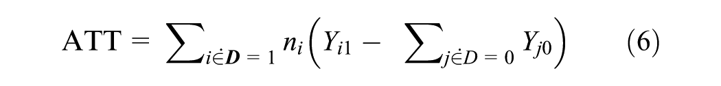
Under these assumptions, the treatment effect for the treated group can be consistently estimated by,

In this formulation, Wij indicates the relative importance attributed to each control unit j when matched with treated unit i while ni reflects the cumulative weight used in constructing the final estimate for the treated group. Yi1 and Yj0 correspond to the observed outcomes for treated and control individuals, respectively.
There are numerous potential matching strategies. To link the collection of untreated observations to each participant in each scheme, proximity criteria, neighbourhoods, and appropriate weight functions must be defined.
Treatment Effect on the Treated (ATT) Using Nearest Neighbour Matching (NNM)
The nearest-neighbour matching (NNM) estimator and the Gaussian kernel estimator are employed without imposing any limitations on the region of common support. For the nearest-neighbour matching estimator, utilizing the notation from equation (5), we set Wij=1, as each treated individual is paired with the closest non-treated counterpart.
Treatment Effect on the Treated (ATT) Using Kernal Matching (KM)

For the Gaussian kernel estimator, each treated unit i's outcome is contrasted with a kernel-weighted average of all untreated individuals' outcomes. The weight given to an untreated unit j is proportional to the proximity of i and j's propensity scores. The outcome Yj0 is formally weighted by Wij=
Employing both Nearest Neighbour Matching (NNM) and Kernel Matching (KM) methods constitutes a robust and complementary strategy for causal inference. NNM provides a straightforward and intuitive matching framework by pairing each treated unit with the nearest untreated unit, thereby reducing variance but potentially introducing bias if the matches are suboptimal. Conversely, KM utilizes all control observations, weighted by their proximity in propensity scores, thus mitigating bias but possibly increasing variance. The application of both methods facilitates the validation of treatment effect consistency across varying assumptions and match qualities, thereby enhancing the credibility and robustness of the causal estimates.
Step 4: Post-Matching Analysis
To determine whether significant differences exist, we evaluate the mean values of the outcome variables for both groups following the establishment of matched treatment and control cohorts.
Regional Heterogeneity Model
This study further utilizes a binary logistic regression model (Greene, 2018) to analyze the regional disparities in rural non-farm employment (RNFE) within Uttar Pradesh (UP). In this framework, the dependent variable is dichotomous, taking the value of 1 if an individual (or household) is involved in non-farm work, and 0 if otherwise. The model is structured as follows:

Where, Yi is the dependent variable, Xi is explanatory variables, Ri Regional dummy variables (Western, Eastern, Central, and southern regions of UP) and εi Error term. A key motivation for this model arises from the observed regional disparity in poverty incidence across Uttar Pradesh. Notably, Western UP exhibits a significantly lower incidence of rural poverty compared to other regions. This empirical observation raises important questions about the role of structural factors, particularly access to non-farm employment, in influencing income levels and poverty outcomes.
By incorporating regional fixed effects in the logit model, we aim to isolate and quantify the effect of regional location on the probability of engaging in non-farm employment, after controlling for individual-level characteristics. This approach allows us to test the hypothesis that higher engagement in RNFE in Western UP is one of the explanatory factors behind its relatively lower poverty levels. The model thereby facilitates a deeper understanding of how regional economic structures and opportunities shape rural livelihoods and poverty dynamics.
Descriptive Analyses
Trend of Poverty in Rural Uttar Pradesh
Monthly household expenditure data from the Employment and Unemployment surveys of the NSSO and Periodic Labour Force Survey (PLFS) were used to estimate the Poverty Head Count Ratio (PHCR), or the percentage of persons living below the poverty line. This is done because it allows us to calculate the poverty of individuals by employment sector (Farm and Non-farm), which is not achievable using data from consumer spending surveys. We used the planning commission's estimated minimum threshold monthly per capita consumption expenditure (MPCE) levels for 2004–2005 and 2009–2010. Additionally, the 2019–20 threshold poverty lines were determined by properly adjusting the 2009–2010 poverty line using the 2019–20 Consumer Price Index for rural labour. It is noteworthy to mention that according to the Tendulkar method, the updated poverty line expenditure for rural Uttar Pradesh in 2004–05, 2009–10 and 2019–20 was Rs. 435.1, Rs. 663.7 and 1131.76, respectively.
The empirical evidence drawn from PLFS 2019–20 and earlier NSSO rounds reveals a discernible relationship between non-farm employment and poverty in rural Uttar Pradesh. Table 2 of the study demonstrates that the poverty rate among rural non-farm workers stands at 30.14%, which is considerably lower than the 40.35% recorded for farm workers. This trend is evident across gender categories, with female non-farm workers experiencing a notably reduced poverty rate of 25.9%, in contrast to their agricultural sector counterparts, who face a rate of 40.7%. The greater income stability and wage benefits associated with non-farm employment likely account for this difference. These results suggest that non-farm job opportunities can play a crucial role in alleviating rural poverty by providing more consistent and lucrative income sources.
Poverty Among Rural Workers in Uttar Pradesh*, 2019-20.
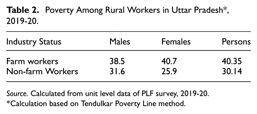
Source. Calculated from unit level data of PLF survey, 2019-20.
Calculation based on Tendulkar Poverty Line method.
However, as illustrated in Figure 2, the relationship is not uniformly linear across different states of India. States such as Kerala, Punjab, and Himachal Pradesh demonstrate both a high proportion of non-farm income and low levels of poverty, suggesting successful structural transformation and the availability of high-quality non-farm employment opportunities. Conversely, states like Assam and Odisha present a paradox where high shares of non-farm income coexist with elevated poverty levels, likely due to the prevalence of low-paying or informal non-farm employment. Thus, while non-farm work is generally associated with poverty reduction, its effectiveness is critically contingent upon the quality of employment and regional socio-economic conditions.
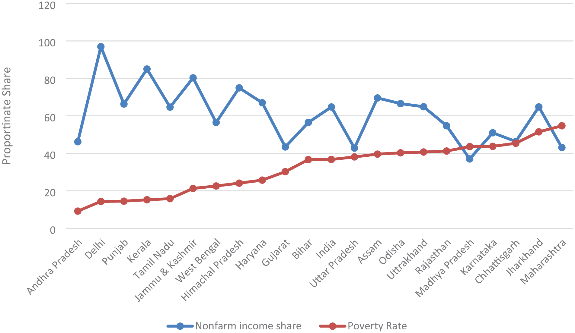
Proportionate share of non-farm income and poverty rate in various states of rural India.
The regional dimension within Uttar Pradesh further underscores the disparate impact of non-farm employment on poverty alleviation. Table 3 illustrates significant variation in poverty trends across the four major regions of the state-Western, Central, Eastern, and Southern Uttar Pradesh-over the three survey rounds from 2004–05 to 2019–20. Western Uttar Pradesh exhibits the most favorable outcomes, with poverty declining steadily from 42.27% in 2004–05 to 24.72% in 2019–20. This stands in stark contrast to Central and Eastern Uttar Pradesh, where poverty rates in 2019–20 remained high at 47.11 and 45.21%, respectively. The Southern region, while still lagging, demonstrated an improvement from 45.17% in 2009–10 to 38% in 2019–20. These findings suggest that the advantages of non-farm employment are not uniformly distributed across the state. Western Uttar Pradesh’s proximity to urban centers and superior infrastructure may have facilitated more productive non-farm opportunities, whereas in other regions, such opportunities may be limited or poorly remunerated. The data clearly highlight the necessity for regionally tailored policy interventions that address structural bottlenecks and enhance access to high-quality non-farm employment in the lagging regions.
Incidence of Rural Poverty in Uttar Pradesh and Different Regions of the State since 2004-05*.
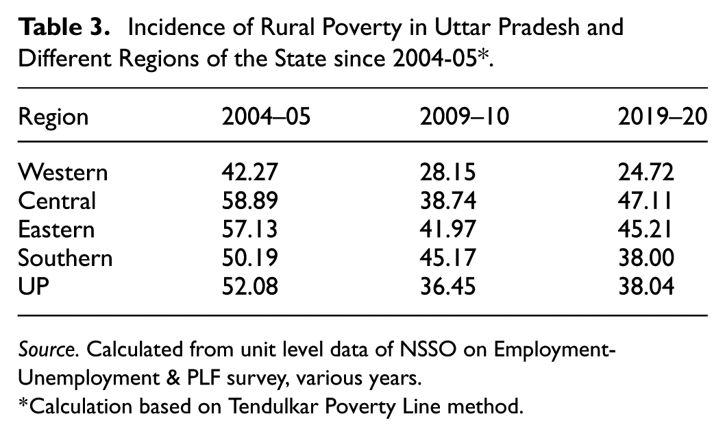
Source. Calculated from unit level data of NSSO on Employment-Unemployment & PLF survey, various years.
Calculation based on Tendulkar Poverty Line method.
Non-Farm Employment Growth and Wage Income Sources
Trends in the structure of rural employment and wage patterns further substantiate the conclusion that non-farm employment has become a pivotal factor in driving rural income growth and alleviating poverty in Uttar Pradesh. Figure 3 offers a longitudinal perspective on the transformation of rural employment, illustrating a consistent decline in agricultural employment alongside a corresponding increase in non-agricultural work since the early 1990s. This transition has been accompanied by a notable disparity in income across various employment types, as evidenced in Tables 4 and 5.
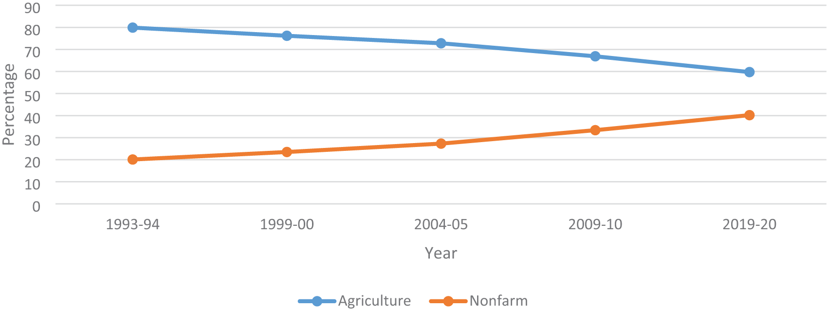
Share of agricultural and non-agricultural employment in rural UP since 1990s.
Workers’ Average Monthly Income by Various Employment Status in Rural Uttar Pradesh (Current Weekly Status), 2019–20.

Source. Calculations derived from unit-level data of PLFS as cited in Hashmi (2025).
Comparison of Daily Real Wages/Income in Farm and Non-Farm Sectors in Uttar Pradesh Between 2009–10 and 2019–20 (In 2009–10 Prices).
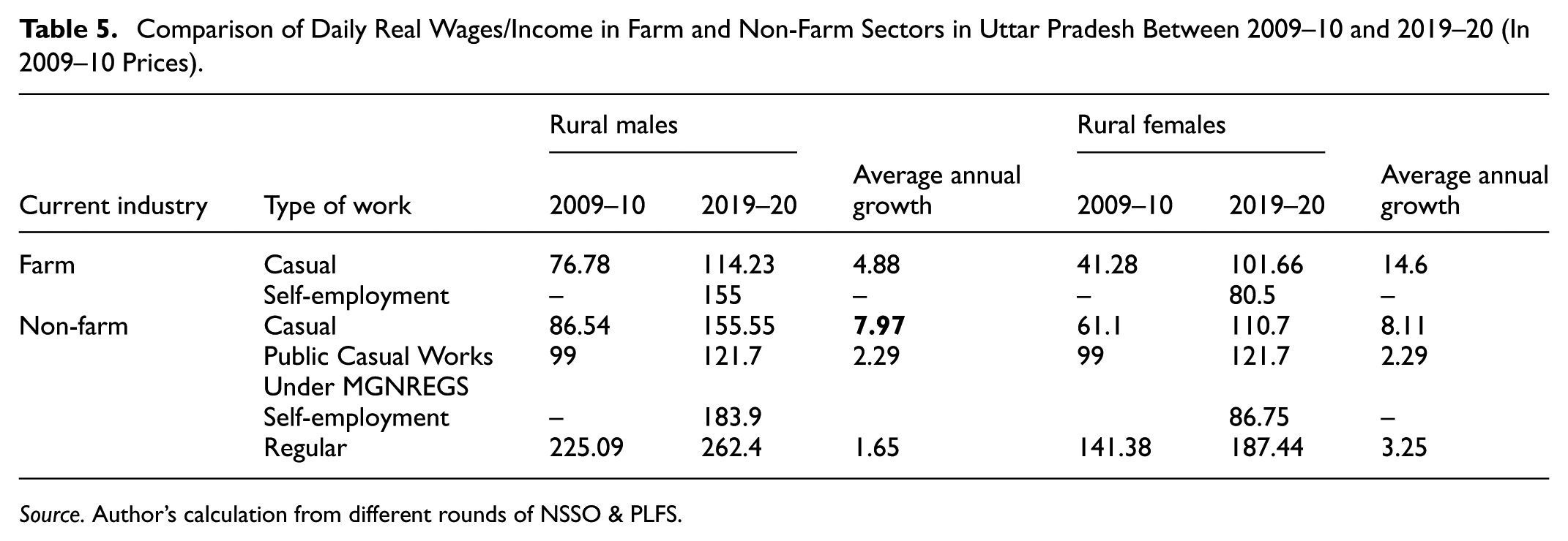
Source. Author’s calculation from different rounds of NSSO & PLFS.
The NSSO categorizes rural economic activities into three primary forms of employment: self-employment, regular wage or salaried employment, and casual or daily wage labour. In 2019–20, the average monthly income for agricultural wage laborers was ₹5,495, whereas non-farm casual workers earned ₹7,440, and self-employed non-farm workers received ₹8,577. Regular non-farm workers earned even higher wages, averaging ₹11,914 per month, indicating the superior income potential available outside the agricultural sector (Table 4). Furthermore, real wage trends over the past decade highlight the increasing appeal of non-farm employment. Casual non-farm wages for rural males and females rose at annual rates of 7.97% and 8.11%, respectively. In contrast, regular employment exhibited sluggish wage growth, and although agricultural wages increased, they remained the lowest within the rural wage hierarchy. Notably, the exceptionally high growth in farm wages for females (14.6%) appears to be an indirect consequence of increased male migration to non-farm work, which has led to labor shortages and subsequently driven up wages in the agricultural sector (Table 5). These wage dynamics collectively suggest that non-farm employment not only offers relatively better income but also stimulates broader labor market adjustments that enhance income conditions in rural areas.
In conclusion, the analysis elucidates a nuanced yet coherent narrative: non-farm employment has emerged as a pivotal mechanism for alleviating rural poverty in Uttar Pradesh. Nevertheless, the magnitude of its impact is influenced by regional disparities, gender differences, and the quality of available employment. These findings underscore the necessity for targeted policy interventions aimed at expanding and enhancing non-farm employment opportunities, particularly in the economically disadvantaged regions of the state.
Results
The following are the empirical assessments of RNFE’s impact on per capita income and consumer expenditures: Prior to the impact analysis, propensity scores for the treatment variables were determined. A probit model was employed to estimate the likelihood of selecting an RNFE and used for generating propensity scores (Table 7). Figure 4 illustrates the common support conditions. Table 8 shows the post-matching balancing of the variables. Table 9 presents the Rosenbaum sensitivity analysis for robustness. Ultimately, the nearest neighbour matching (NNM) and kernel-based matching (KBM) methods were utilized to gauge the effects of RNFE on PCI and MPCE (Table 10).

Propensity score distribution and common support for propensity score estimation (outcome variable, PCI & MPCE).
Determinants of RNFE Participation
It is generally assumed that engagement in agricultural or non-agricultural employment is influenced by internal dynamics within the rural economy. Individuals working in agriculture do not constitute a random selection from the broader labour pool; rather, they tend to self-select into sectors based on largely unobservable traits such as personal preferences, physical capacity, skillsets, or desired working conditions. In this study, the effect of rural non-farm employment (RNFE) is assessed using data drawn from the same rural environment, which helps to partially account for the selection bias associated with these unobserved factors. Meanwhile, differences in observable characteristics between those engaged in farm and non-farm work can be addressed through the use of matching methods.
Table 6 displays the descriptive statistics and a comparison of the outcome variables. The treatment groups demonstrated superior performance compared to the control group in both outcome variables, with higher earnings and more time spent working. This disparity was particularly evident in the income category. Individuals engaged in non-farm employment earn an average of Rs 1,867 per month per capita, whilst those in farm employment earn Rs 1,576. Both income and expenditure variables exhibit high standard deviations, with income showing greater variability than expenditure. Regarding workers, the demographic characteristics show that the treated person’s gender, age, and household size were more or less similar to those in the control group (Table 6). In addition, the treated individuals had completed more years of general education than the control group, although both groups displayed the same trends for technical education. It is also clear that the treated group of workers was younger than the control group was. Scheduled caste individuals were more concentrated in the treated group, whereas ST, OBC, and Others were broadly distributed equally in both the treated and non-treated groups. Muslims have a slightly higher representation in the treated group than in the non-treated group, according to the occupational distribution of various religions.
Mean Attributes for the Probable Control and Treated Groups of Workers.

Source. Author ‘s Own calculation from PLFS, 2019–20,
Standard deviation in parenthesis.
According to geographical distribution, there was little variation in each location between the proportion of workers who received treatment and those who did not. The monthly per capita income (PCI) for the treated group is clearly larger than the non-treated groups, and the MPCE is moderately higher in the treated group.
The choice of conditioning variables to be incorporated into Xi in order to estimate the propensity score is the next problem. We take into account all individuals’ time-constant and time-variable characteristics, such as gender, age, education, caste, religion, and geographic distribution, which were unaffected by the treatment group.
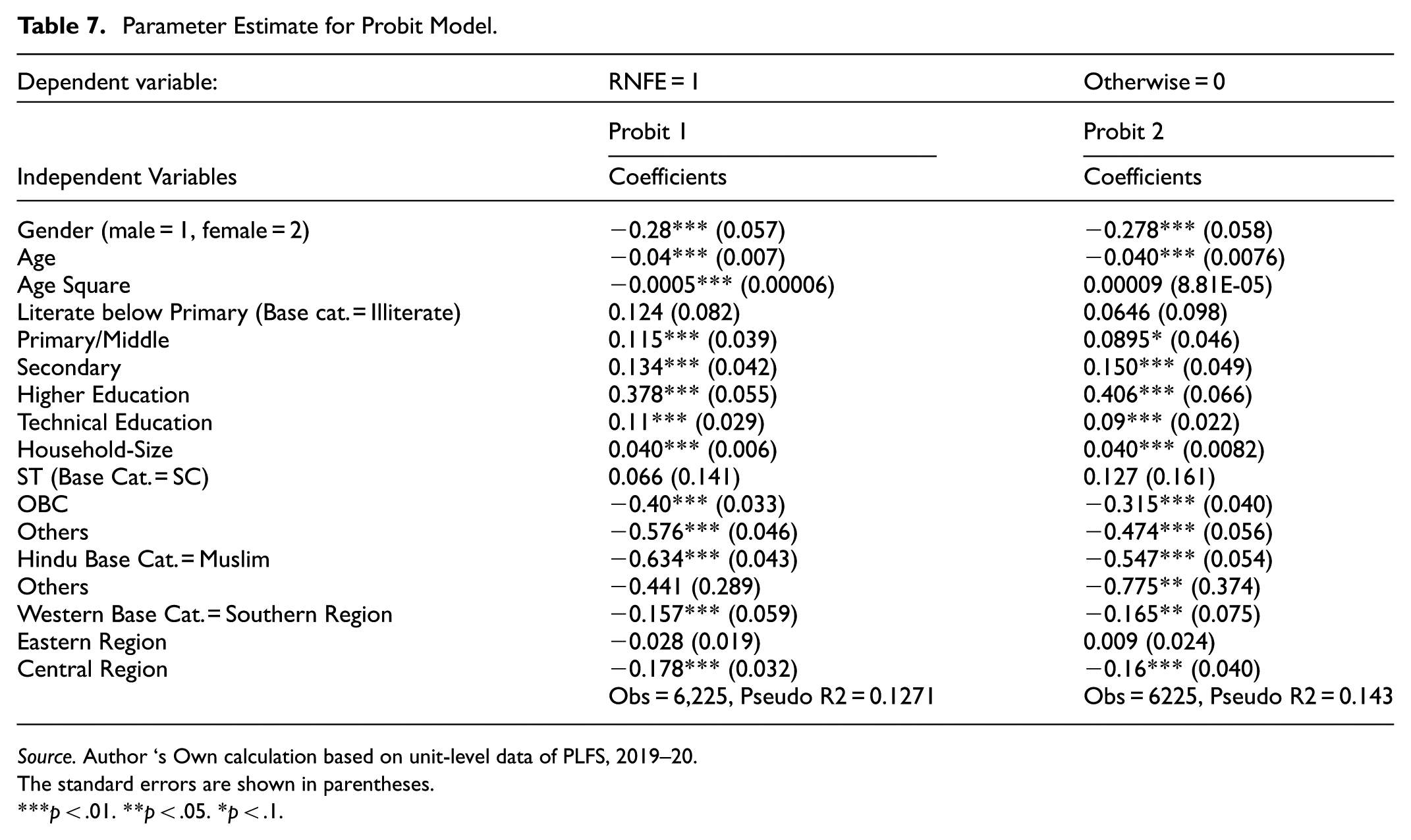
The probit regression findings of the propensity score are shown in Table 7 and correspond to Equation (1) in the preceding section. The estimation results indicate a gender bias in employment opportunities, favoring males over females in non-farm activities. Individuals with at least a primary level of education are more inclined to seek employment outside the agricultural sector. Moreover, those with higher levels of education, particularly at the secondary and tertiary stages, tend to have a greater likelihood of being employed in non-farm occupations. The estimated coefficients for caste and religious identity indicate that Muslims have a higher probability of participating in non-agricultural work compared to Hindus. Similarly, workers belonging to Scheduled Castes are more likely to be engaged in non-farm employment than those from Other Backward Classes (OBC) and Others.
Parameter Estimate for Probit Model.
Source. Author ‘s Own calculation based on unit-level data of PLFS, 2019–20.
The standard errors are shown in parentheses.
p < .01. **p < .05. *p < .1.
Workers in the southern region are more likely to work in off-farm activities according to the coefficient of the regions. Similarly, Table 7 also displays the probit model used to determine the p-score for the outcome variable income.
Although the estimated propensity score model yields a relatively low pseudo R2, this is neither unexpected nor problematic in the context of matching. In PSM, the primary aim is not to achieve high predictive power, but rather to balance covariates across treated and control groups. A low pseudo R2 suggests that the observed covariates do not perfectly separate the treated and control observations, which supports the existence of common support and enhances the credibility of comparisons. This is confirmed visually in Figure 4, where the distribution of propensity scores shows substantial overlap between the two groups. Thus, the low pseudo R2 complements the graphical evidence of good matching quality and supports the appropriateness of the matching strategy.
Regional Heterogeneity
Table 8 presents the predicted probabilities of rural non-farm employment (RNFE) across four regions of Uttar Pradesh (UP), as estimated from a binary fixed effect model that includes regional dummy variables to assess regional variation. To account for unobserved regional characteristics like infrastructure, market access, and socio-economic development that might affect RNFE participation, the model includes regional dummy variables for Western, Eastern, Central, and Southern UP. By integrating these fixed effects, the model distinguishes the influence of regional location on RNFE involvement while controlling for individual-level factors such as gender, education, caste, religion, and age. The findings indicate predicted RNFE participation probabilities of 43% for Eastern, 42% for Southern, 40% for Western, and 35% for Central UP.
Predicted Probabilities of Non-Farm Employment in Four Regions of Uttar Pradesh.

Source. Author ‘s Own calculation based on unit-level data of PLFS, 2019–20.
These statistics suggest that RNFE involvement is fairly consistent across regions, with only slight differences. Interestingly, Western UP, despite having a lower poverty rate, does not show the highest RNFE probability, suggesting that the quality, stability, and income potential of non-farm employment, rather than mere participation, might better explain regional poverty disparities. This suggests that in regions like Western UP, non-farm jobs might be more profitable or stable, thus having a greater impact on poverty reduction despite similar participation levels. On the other hand, Eastern and Southern UP, which have the highest RNFE probability, still experience high poverty levels, indicating that non-farm jobs there might be less stable, poorly paid, or insufficient to lift households out of poverty, likely due to deeper structural issues such as landlessness, institutional deficits, agricultural productivity, or low educational attainment. This underscores the significance of structural and institutional factors in shaping rural livelihoods and emphasizes the need to look beyond participation rates to evaluate the true impact of RNFE on poverty alleviation.
Matching Quality and Balance Tests
Figure 4 illustrates the common support condition for the outcome variables, Per Capita Income (PCI) and Monthly Per Capita Consumption Expenditure (MPCE), by showing the distribution of propensity scores for both the treated group (those engaged in RNFE) and the control group (non-RNFE). The noticeable overlap between the two distributions confirms that the common support requirement is satisfied, which is essential for the credible estimation of treatment effects. A few treated observations fall outside this overlapping region and are therefore excluded from the analysis to avoid making inferences beyond the range of the observed data. This exclusion enhances the internal validity of the propensity score matching (PSM) approach and improves the robustness of the Average Treatment effect on the Treated (ATT) estimates.
As suggested by Leuven and Sianesi (2003), the matching process is confined to the region of common support, eliminating treated units whose propensity scores lie beyond the minimum or maximum values observed in the control group. Figure 4 underscores the importance of adhering to the common support condition and demonstrates the contrast in the propensity score distributions between individuals engaged in non-farm and farm employment, emphasizing the role of careful matching in avoiding inappropriate pairings.
The balance diagnostics presented in Table 9 reveal that the propensity score matching process, which utilizes the nearest neighbor technique, has successfully balanced most of the observed covariates between the treated group (RNFE participants) and the matched control group (non-RNFE). Key demographic and socio-economic factors, including age, gender, education, caste, religion, and region (with one exception), show no statistically significant differences after matching, indicating a strong balance of covariates (In the case of the outcome MPCE, none of the covariate variables demonstrated statistical significance, as illustrated in Appendix I.). The Central region is the only exception, remaining slightly imbalanced (p = .045), which suggests some residual regional heterogeneity that might affect treatment outcomes. This limitation is recognized, and future studies might address it through region-specific matching. Notably, outcome variables such as monthly per capita income (PCI) and consumption (MPCE) continue to show significant differences post-matching, as anticipated, since the treatment effect is assessed based on these outcomes. To further evaluate the robustness of the estimated treatment effects against unobserved confounding, Rosenbaum’s sensitivity analysis was conducted. The findings reveal that the estimated ATT remains statistically significant even with moderate levels of hidden bias (Γ > 1.5), indicating that the conclusions derived from the PSM are resilient to potential unobserved heterogeneity. This enhances the credibility of the causal claims, while acknowledging that no matching method can completely eliminate the impact of unmeasured confounders.
Summary Matching Variables of Treated Individuals (RNFE) and Control Groups (Outcome Variable, PCI), 2019–20.

The t-test for balance checking, as reported in the fourth column, utilized post-matching data obtained through the nearest neighbourhood method to compare means. The corresponding P-values are enclosed in parentheses.
Rosenbaum’s Sensitivity Analysis
To evaluate the robustness of the estimated treatment effects against possible hidden biases, Rosenbaum's sensitivity analysis was applied to the results obtained from the propensity score matching (PSM) approach. Table 10 explores how the estimated impact changes with varying degrees of unobserved confounding, represented by the sensitivity parameter Γ, which reflects the odds of treatment assignment differing due to unmeasured factors.
Rosenbaum Sensitivity Test Results.
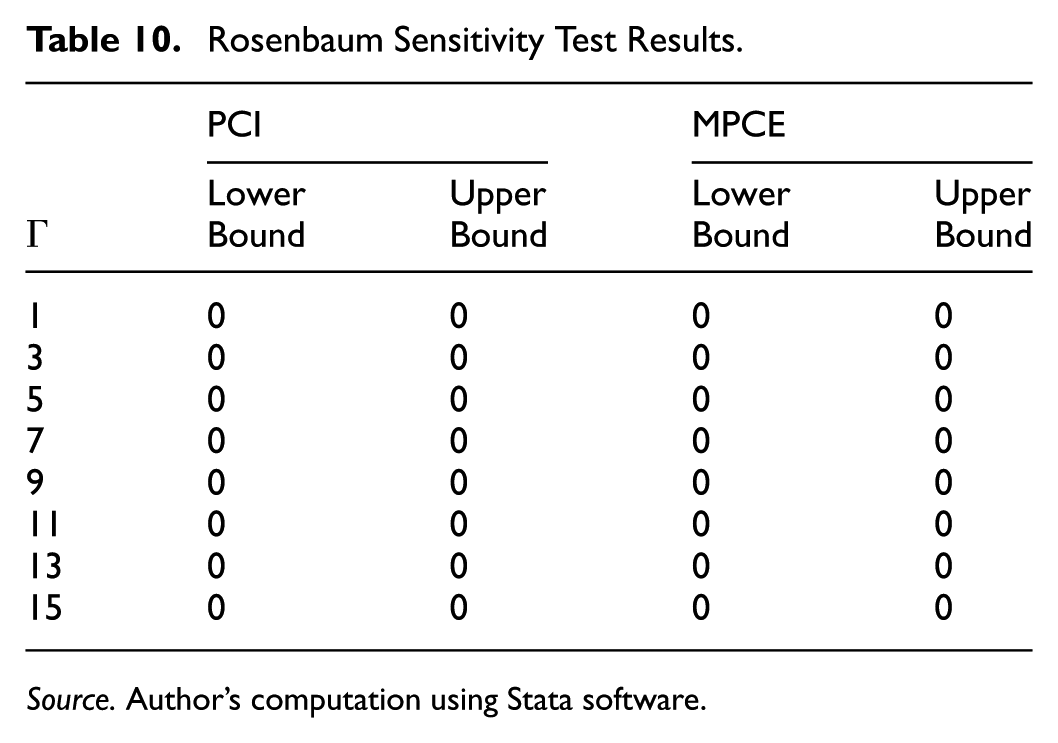
Source. Author’s computation using Stata software.
Across all tested values of Γ, the estimated treatment effect for both outcome indicators, per capita income (PCI) and monthly per capita consumption expenditure (MPCE), remained consistently at zero, with no variation in the lower and upper bounds. This outcome indicates that the estimated effects are not sensitive to the presence of substantial hidden bias. The application of Rosenbaum’s method to PLFS 2019–20 data supports the conclusion that the observed causal relationships between non-farm employment and household welfare indicators are reliable, even when accounting for hypothetical unmeasured confounders. Consequently, these results reinforce the credibility of the PSM-based findings.
Average Treatment on the Treated (ATT)
Table 11 presents the estimated Average Treatment Effect on the Treated (ATT) of rural non-farm employment (RNFE) on two key indicators of household welfare: Monthly Per Capita Income (PCI) and Monthly Per Capita Consumption Expenditure (MPCE). To enhance the reliability of the estimates and address potential biases arising from non-random selection into non-farm employment, the analysis applies two commonly used matching methods—Nearest Neighbor Matching (NNM) and Kernel-Based Matching. The results indicate that RNFE has a positive and statistically significant effect on both income and consumption, underscoring its meaningful contribution to improving rural household welfare.
Average Treatment Effect (ATT) of RNFE in Uttar Pradesh, 2019–20.

Note. Z-value in parenthesis.
Significant at 1% Level.
Using the nearest neighbor matching method, households involved in RNFE report a monthly per capita income increase of 412.78 INR compared to similar agricultural households, with a strong z-statistic of 8.36, significant at the 1% level. The kernel-based matching method provides a consistent estimate of 416.80 INR, with a z-value of 8.29, further supporting the reliability of the income increase associated with non-farm employment. A similar trend is observed for consumption. Households engaged in RNFE see a rise in monthly per capita consumption of 97.12 INR under the nearest neighbour approach (z = 3.85), while the kernel-based matching estimates a similar effect of 97.54 INR (z = 3.35). These results suggest that participation in RNFE not only boosts income levels but also enhances household welfare through increased consumption. Both matching algorithms utilize 2,621 treated observations (households engaged in RNFE) and 3,604 matched controls (households not engaged in RNFE), ensuring a sufficiently large and balanced sample for credible inference. The close alignment of results across both methods further confirms the robustness and internal validity of the estimated treatment effects. Considering that the monthly per capita income in rural UP is approximately Rs.1,696, the difference between agricultural and non-farm employment is significant. Compared to farm activities, individuals working in rural non-farm activities earn 28.68% more per month. In rural UP, a worker’s monthly per capita consumer spending is 7% higher if they are employed in non-farm activities rather than farming. These findings support the hypothesis that RNFE serves as a crucial avenue for income diversification and poverty alleviation in rural Uttar Pradesh. The positive effects on both income and consumption suggest that promoting non-farm employment can play a vital role in improving rural living standards and reducing regional economic disparities.
Discussion on Findings
This study offers empirical insights into how rural non-farm employment (RNFE) affects household welfare enhancement in Uttar Pradesh. Utilizing propensity score matching (PSM) to mitigate selection bias in observational data, the research demonstrates that participation in RNFE is associated with significantly increased monthly per capita income (PCI) and consumption expenditure (MPCE). These results are consistent across different matching algorithms and remain robust through essential balance and sensitivity tests, including Rosenbaum’s bounds. The findings affirm that RNFE serves as a vital supplementary source for sustaining rural livelihoods, particularly in areas where agricultural employment is either inadequate or unstable. The income and consumption improvements seen among RNFE participants are considered absolute enhancements, not just relative ones, indicating real increases in household resources rather than merely improved standing compared to others. However, a detailed examination of the data shows that many households involved in RNFE, especially in less developed regions, still fall below or hover just above the poverty line. This implies that while RNFE does help alleviate poverty, it often provides only marginal economic security rather than a complete escape from poverty. Therefore, the poverty-reducing effect of RNFE is significant but partial, and it heavily depends on the type, stability, and remuneration level of the non-farm work.
While this study provides valuable insights, it is constrained by its reliance on cross-sectional data, which limits the ability to examine long-term welfare trajectories or dynamic labour market transitions. Future research should therefore employ longitudinal or panel datasets to capture the persistence and evolution of welfare effects associated with RNFE participation over time. Moreover, causal inferences drawn from the present analysis should be interpreted with caution due to potential unobserved heterogeneity- such as entrepreneurial aptitude, risk preferences, or access to informal networks- that may simultaneously influence employment choice and welfare outcomes. To address these challenges, subsequent studies could adopt advanced causal identification strategies, including instrumental variable approaches, fixed-effects panel models, or experimental and quasi-experimental designs, to more rigorously assess the sustained impact of RNFE on poverty reduction and household well-being.
When examined from a comparative perspective, the findings are consistent with research conducted in other Indian states and countries within the Global South. Specifically, the results broadly align with evidence from other Indian states and global South contexts. Research in Bihar and West Bengal has underscored the importance of the Rural Non-Farm Employment (RNFE) in boosting rural incomes and stabilizing consumption, particularly through sectors like construction, trade, and informal services (Himanshu et al., 2013; Choithani et al., 2021). This trend is also evident globally, as seen in countries such as Bangladesh (Hossain, 2019), Kenya (Reardon et al., 2006), Uganda (Asiimwe et al., 2025), Ghana (Zereyesus et al., 2017), and Vietnam (Imai et al., 2015), where diversification into non-farm activities plays a crucial role in improving household welfare. However, in Uttar Pradesh, the advantages of RNFE seem relatively limited, possibly due to the lower productivity and informality prevalent in much of the state’s non-farm sector.
Significantly, the study highlights regional variations in participation in and the impact of Rural Non-Farm Employment (RNFE). For instance, the incidence of poverty is lowest in Western Uttar Pradesh, a comparatively more developed area; however, the likelihood of engaging in RNFE is not markedly higher than in other regions, such as Southern or Eastern Uttar Pradesh. This indicates that while RNFE is advantageous across regions, the motivation for participation varies: in the more developed west, it may be driven by opportunities and linked to higher-quality employment (e.g., trade, services), whereas in less developed regions, it is often driven by distress and concentrated in low-wage sectors like construction. This suggests that the same employment category (RNFE) may differ significantly in its contribution to well-being, contingent upon the local economic context, infrastructure, and institutional support. Overall, the findings emphasize that RNFE is an important yet insufficient tool for poverty alleviation. Its impact is influenced by regional disparities, the structure of rural labor markets, and the quality of employment opportunities. Consequently, a uniform approach to promoting RNFE would be inadequate; instead, policies must be tailored to local conditions and focused on enhancing the quality, security, and inclusiveness of non-farm employment opportunities.
Conclusion and Policy Recommendations
This study advances the empirical comprehension of rural livelihoods by assessing the causal effects of rural non-farm employment (RNFE) on household welfare in Uttar Pradesh. By employing propensity score matching on nationally representative cross-sectional data, the study demonstrates that engaging in RNFE is linked to enhanced household economic outcomes, notably increased per capita income and consumption expenditure. The results affirm that RNFE is vital in strengthening the economic resilience of rural households in a region characterized by significant structural inequalities and agricultural distress. However, these gains, while significant, are insufficient to completely alleviate poverty for all households. RNFE provides absolute improvements in income and consumption, yet many beneficiaries remain near or just above the poverty threshold. This highlights the dual nature of RNFE: it acts both as a buffer against income shocks and a potential stepping stone for upward mobility, but its effectiveness is constrained by the type and quality of employment available, which is often informal, low-paying, and precarious. The analysis also underscores regional variations in both poverty levels and employment structures. While Western Uttar Pradesh exhibits lower poverty levels overall, the likelihood of RNFE participation is not significantly higher than in other regions. This suggests that the motivations for and outcomes of RNFE participation vary across regions, being more opportunity-driven in developed areas and distress-driven in less developed ones. These findings emphasize the importance of regional customization in policy design.
From a policy perspective, the results indicate that merely expanding RNFE opportunities is insufficient. To transform RNFE into a more effective poverty-reduction strategy, the quality and sustainability of non-farm employment must be addressed. Policymakers should prioritize: - Investment in rural infrastructure, such as roads, electricity, and digital access, that supports non-farm enterprises development and connectivity to markets. Skills training and vocational education, particularly in sectors with high employment potential such as construction, transport, rural services, and agro-processing. - Credit access and enterprise support, especially for marginalized groups such as women, Dalits, and Muslims, who often face exclusion from formal labor and financial markets. - Targeted support in underdeveloped regions, where RNFE is largely distress-driven, to enhance both the availability and desirability of rural employment.
In conclusion, while RNFE offers a significant pathway towards poverty alleviation in rural Uttar Pradesh, its transformative potential depends not only on job creation but also on job quality, inclusiveness, and regional appropriateness. Well-targeted public investment and inclusive economic policy will be essential to ensuring that RNFE becomes a driver of rural development rather than a coping mechanism for structural deprivation.
Footnotes
Appendix
Summary Matching Variables of Treated Individuals (RNFE) and Control Groups (Outcome Variable, MPCE), 2019–2020.

| Demographic variables | Mean of control group (farm)-matched | Mean of treated group (non-farm) | t-value for differences in matched and control groups |
|---|---|---|---|
| Gender (male = 1, female = 2) | 0.91 | 0.91 | −0.42 (0.672) |
| Age | 34.23 | 34.35 | 0.42 (0.674) |
| Age Square | 1289.10 | 1295.90 | 0.34 (0.736) |
| Below primary | 0.03 | 0.03 | 0.58 (0.564) |
| Primary | 0.35 | 0.35 | −0.48 (0.631) |
| Secondary | 0.29 | 0.29 | −0.43 (0.67) |
| Higher Education | 0.12 | 0.12 | −0.06 (0.956) |
| Technical education | 1.07 | 1.12 | 1.68 (0.094) |
| Household Size | 5.57 | 5.56 | −0.16 (0.87) |
| Scheduled Tribe | 0.01 | 0.01 | −0.54 (0.589) |
| Other Backward Caste | 0.51 | 0.52 | 0.87 (0.387) |
| Others | 0.14 | 0.13 | −1.2 (0.23) |
| Muslim | 0.17 | 0.18 | 0.43 (0.667) |
| Others | 0.00 | 0.00 | −0.27 (0.789) |
| Western Region | 0.35 | 0.36 | 0.14 (0.887) |
| Central Region | 0.16 | 0.15 | −0.85 (0.394) |
| Eastern Region | 0.42 | 0.43 | 0.35 (0.725) |
| Monthly Per Capita Expenditure(MPCE) | 1455.4 | 1481 | 9.12 (0.00) |
The t-test for balance checking, as reported in the fourth column, utilized post-matching data obtained through the nearest neighborhood method to compare means. The corresponding P-values are enclosed in parentheses.
Acknowledgements
The author gratefully acknowledges Dr. M. D. Azharuddin Akhtar, Associate Fellow at the Institute for Human Development, New Delhi, for his valuable guidance during the preparation of this manuscript.
Ethical Considerations
The article did not involve any human participants.
Author Contributions
The author conceived the idea, performed the calculations, collected secondary data, and validated the analytical methodologies.
Funding
The author received no financial support for the research, authorship, and/or publication of this article.
Declaration of Conflicting Interests
The author declared no potential conflicts of interest with respect to the research, authorship, and/or publication of this article.
Data Availability Statement
The authors can provide data and materials upon request.