Sage Journals: Discover world-class research

Abstract

The study examines the cyclical relationship between the stock market and business cycles in India, utilizing monthly data from April 1996 to March 2024. It incorporates the combined market capitalization of the BSE and NSE, broad money supply (M3), the S&P 500 and the Index of Industrial Production (IIP) as a proxy for the business cycle. The cycles were computed using the Hodrick-Prescott filter and the Bry-Boschan algorithm to identify the turning points. This study integrates turning-point analysis with the Structural Vector Autoregression (SVAR) framework for high-frequency data, providing evidence on the transmission of financial shocks to real activity. The findings reveal that the stock market exhibited more pronounced fluctuations and shorter durations compared to business cycles. A bidirectional relationship was observed between M3 and business cycles. Interestingly, the global S&P 500 exhibited some alignment with business cycles only during the crisis period. There is growing recognition that financial variables are procyclical and share a close relationship with macroeconomic indicators. Consistent with this view, the lead-lag analysis revealed that the stock market led business cycles by 1 to 3 months, highlighting its role as a leading indicator. Moreover, SVAR analysis confirmed a long-run positive relationship among the BSE, NSE, M3, and business cycles. The findings underscore the need for financial deepening and stabilizing the capital market to ensure long-term economic growth.

JEL Classification: E32, E52, G2, O1

Plain Language Summary

Does the Stock Market Lead the Economy? A Study of the Stock Market and Business Cycles in India

The Indian economy and financial markets experience fluctuations; however, it remains unclear whether these financial markets serve as early warning indicators. The study used the stock market (BSE and NSE) and the broad money supply (M3) as indicators, along with a US-based indicator (S&P 500). Industrial production (IIP) was employed as a proxy for real economic activity. We used monthly data and applied the HP filter and SVAR to identify patterns in these cycles. The results show that the stock market often leads business cycles by 1 to 3 months. Similar co-movements were seen during the 2008 financial crisis and COVID-19 among the stock market, money supply, and business cycles. However, the S&P 500 did not show any meaningful relationship with Indian economic activity. SVAR also confirmed a long-run relationship between them. The Granger causality test reveals a two-way link between money supply and growth. These findings suggest that fluctuations in financial markets can help predict slowdowns and economic changes. Policymakers can use stock market trends to prepare for economic shifts.

Keywords

stock market business cycles broad money supply SVAR HP filter

Introduction

Financial development and economic growth are closely related concepts. A strong financial system comprising money and capital markets plays a significant role in stabilizing macroeconomic indicators, as suggested by King and Levine (1993). Johnson (1983) suggests, “The stock markets are a complex of institutions and mechanisms through which funds for purposes longer than one year are pooled and made available to businesses, government, and individuals and through which instruments already outstanding are transferred. The stock markets are well organized and are local, regional, national and worldwide in scope.” A healthy stock market indicates an optimistic attitude among investors about future economic prospects. It may also see the stock market as a predictor of real business cycles. According to Fischer and Merton (1984), the stock market has historically predicted 6 out of the last 10 recessions. This implies the ability of the stock market to anticipate recessions. The stock market reflects investors’ expectations of future profits and earnings. It has been observed that it’s a leading indicator of real growth, predicting turning points in business cycles; historical crises have shown that even when the economy was in recession, the stock market was upward sloping (Management, 2009). The Bombay Stock Exchange (BSE), established in 1875, is the oldest stock exchange in Asia and the 10^th oldest in the world, with a market capitalization of $1.7 trillion. The National Stock Exchange (NSE) was set up in 1992 in Mumbai and has a market capitalization of $1.65 trillion (Mahajan, 2023), with 2166 companies listed as of December 2023. Both indices are key parameters of financial activity in India, and therefore, the study incorporated them to examine the cyclical dynamics between stock market cycles and business cycles.

Industrial growth is now considered an important indicator of business cycles. Earlier works of literature have also used IIP to represent fluctuations in economic activity (Chitre, 2001). While the role of IIP in GDP has declined, it continues to play an important role in determining the cyclical components of growth. Also, being available at monthly and quarterly data it is appropriate for forecasting economic conditions (Mohanty et al., 2003). During an economic boom, profits are expected to rise, as are stock market prices. However, during the period of economic slowdown, there can be asset liquidation, causing a decrease in stock prices.

India’s GDP growth rate declined post-2017 from 8.17% to 7.17% and continued to fall thereafter. During the COVID-19 pandemic, India’s growth rate further declined to 4.43%, while pre-pandemic it was 7% (Surya, 2024). The stock market also experienced a decline during the period. In time of crisis, investment is expected to decline because consumers fear declining economic activity. However, Shankar and Dubey (2021) found a positive impact of the crisis on trading volume, causing low volatility in the market. The stock market became a hotspot for investors because of the low prices and the expectation of high returns in the near future. A large influence of change in interest rates and monetary policy during the period of the pandemic was observed by Schrank (2024).

Moreover, as believed by Keynesians and monetarists, liquidity strongly influences the stock market. Monetarists believe that increased money supply influences the demand for equity, while Keynesians argue that expansionary monetary policy makes equity more attractive (Tomar & Kesharwani, 2021). Since India is a bank-based economy, this study also incorporated broad money supply (M3) to investigate the cyclical interdependencies with the stock market and real economic activity. Meshram et al. (2020) asserted that the stock market plays a significant role in the overall development of the economy. The developed capital market facilitates access to international funds. It provides a platform for investors interested in buying and selling listed securities. By reducing interest rates, the demand for money increases, and investors invest in the economy, which causes stock prices to increase. The 2008 financial crisis increased the volatility of the stock market due to global trends (Mandal & Bhattacharjee, 2012). This highlights the importance of assessing the effects of the global market on Indian financial markets. Hence, the study incorporated the S&P 500 as a global indicator to investigate the impact of global volatility on the Indian economy.

Identifying the peaks and troughs in the financial market can help us understand the co-movement between the financial cycles and business cycles. Using the Bry-Boschan technique to identify the turning points adds novelty to the research. While the Bry-Boschan technique has been extensively used in the literature, mostly on annual or quarterly data. This study extends its analysis to monthly data and further employs the turning point on the HP filter cyclical component rather than the raw components, reducing the chance of noise and capturing more reliable cycles. However, another question arises: does the financial market lead or lag behind business cycles, and more importantly, by how much time does one lead or lag the other? The study employed cross-correlation to identify the lead-lag relationship. This paper contributes to the existing literature by examining both the co-movements and causality between the stock market cycle and business cycles in India. Furthermore, another important contribution of this paper is to study the relationship between financial market shocks and business cycles using Structural Vector Autoregression (SVAR). While the VAR models are atheoretical, the SVAR allows for imposing the short-run and long-run restrictions. Applied to the cyclical components, this enables us to understand the transmission of financial shocks to real economic activity.

As a result, this study aims to determine the dynamic interactions and potential interconnectedness between real economic activity, equity performance, monetary conditions, and the global market. The Hodrick-Prescott filter was used to extract the cyclical components of the three stock market indices (BSE, NSE, and S&P 500) and the macroeconomic indicators, namely the Index of Industrial Production (IIP) as a proxy for real economic activity and broad money supply (M3). The paper’s structure is as follows: Section 2 provides a comprehensive literature review on the nexus among these variables. Section 3 presents the data and variables utilized. Section 4 describes the econometric methodology. Section 5 presents the findings obtained from the estimation, followed by a robustness test in Section 6. Section 7 discusses the policy implications, and Section 8 summarizes the findings.

Literature Review

To understand the relationship between the stock market development and India’s economic growth, it is essential to review the theoretical and empirical literature.

Theoretical Framework

Supply-Leading and Demand-Following Hypotheses

These hypotheses were formulated by Patrick (1966), who suggested that a causal relationship explains the direction between financial development and economic growth. The supply-leading hypothesis supports that financial development acts as a force of economic growth. As the financial institutions and markets expand their financial services, there’s growth in the real sector. There are several channels through which financial development influences growth: by helping to allocate tangible wealth and resources from savers to investors, increasing the rate of physical capital formation, and providing savings. Schumpeter (1912), Goldsmith (1969), and McKinnon (1973) support the supply-leading hypothesis. The demand-following hypothesis posits that as the real sector develops, the demand for financial services also grows, which means financial developments respond to economic growth (Robinson, 1952). (Atje & Jovanovic, 1993; Levine & Zervos, 1998) suggest a positive and robust impact of the stock market on economic growth, capital accumulation, and productivity, consistent with the supply-leading hypothesis. While Bhullar (2017) found a unidirectional relationship from India’s economic growth to the stock market, supporting the demand following hypothesis.

Stage of Development Theory

The direction of the relationship between financial development and economic growth depends on the stage of development. According to Patrick (1966), in early phases, the supply-leading hypothesis exists; both the savers and investors benefit from developed financial systems. Later, the demand for financial services increases because of economic growth. It can be concluded that in the initial phase of growth, a supply-leading hypothesis exists, and the demand-following hypothesis prevails later.

Financial Liberalization Theory

According to McKinnon and Shaw, financial liberalization is the most effective way to boost economic growth, particularly in developing countries. Gradually, after 1991, India’s government lifted these restrictions through financial reforms. The cash reserve ratios and statutory liquidity ratios declined to 10% over 4 years and 25% within 3 years, respectively. Administrative constraints were eliminated, and new private banks were encouraged. The Securities and Exchange Board of India (SEBI) was set up to regulate the capital market. Consequently, financial deepening increased to 45% in 1990 and to approximately 80% in 2010 (Pal, 2014).

Empirical Literature Review

The stock market and monetary aggregate are often viewed as important drivers of fluctuations in economic growth, particularly in emerging countries like India. Paramati and Gupta (2011) examined the relationship between the monthly indicators like IIP, BSE, and NSE and quarterly GDP from April 1996 to March 1999. Findings revealed a bidirectional causality between IIP, BSE, and NSE. While GDP exhibited a unidirectional relationship with only NSE, no relationship was observed between GDP and BSE. The ECM bound test and Engle-Granger residual test confirmed a long-run relationship between stock market development and economic growth. Palamalai and Prakasam (2014) revealed a long-run positive relationship between the stock market and GDP during June 1991 and June 2013, with the help of ARDL bound testing, and the Granger test confirmed a bidirectional relationship, consistent with the findings of Vinayaranjan et al. (2022). Misra (2018) also confirmed a long-run causality between IIP, BSE Sensex, and money supply, based on VECM results. Similarly, Pandey and Shettigar (2017) observed a positive relationship between monetary supply and IIP during the post-liberalization period. Ghosh and Chhaochhoria (2020) investigated various stock market indicators, such as market capitalization, market turnover and net investments by FIIs and their impact on GDP at constant prices. With the help of ARDL-bound testing, they found that lagged market capitalization had a positive influence on GDP, implying that the stock market had no contemporaneous influence on economic activity. However, in the later period, it led to an increase in new listings, businesses, firms, and investments. Similarly, Sultana et al. (2021) reported a positive influence of stock market indicators on GDP during the period 2003 and 2017, using VAR, aligning with the findings of Ramchandraiah (2024). Keswani et al. (2024) conducted a cointegration analysis and confirmed a positive long-run association between the NSE index and GDP.

Particular emphasis was placed on the country-specific studies, such as Kirankabes and Basarir (2012), who investigated the positive and significant impact of the stock market index ISE 100 on Turkey’s GDP during the period 1998:1–2010:12 using VECM. The Granger causality test revealed one-way causality from the IIP index to GDP. Qamruzzaman and Wei (2018) utilizing ARDL, confirmed the presence of a long-run relationship between the various indicators of financial development, including the stock market and Bangladesh’s GDP during the period from 1980 to 2016. Hoque et al. (2017) re-examined the relationship between stock market development and Malaysia’s economic growth from 1981 to 2016. The study employed ARDL bounds tests, the Granger causality test, and multivariate regression. The ARDL test confirmed a positive short-run and long-run relationship between stock market development and economic growth. The Granger test confirmed a unidirectional relationship from stock market development to economic growth. The bound test also reported a sustained influence of the stock market on economic growth. Chikwira and Mohammed (2023) reported a weak but positive and statistically significant influence of the stock market on Zimbabwe’s economic growth, based on quarterly VAR analysis from 2013 to 2022. Demir (2025), with the help of OLS and panel VECM, found a positive short-run bi-directional relationship between the stock market and economic growth in high-income countries. While a unidirectional relationship was observed between the variables in low- and middle-income countries. However, much of the literature focused on the linear relationships. And given the dynamic nature of these variables, it becomes important to study the cyclical dynamics among them.

Several kinds of literature suggested a dynamic interaction between financial markets and business cycles. Chauvet (2001) reported a significant role of financial cycles in driving fluctuations in economic output, especially during periods of economic fluctuations. Claessens et al. (2011) revealed that output cycles were more synchronized with credit cycles than cycles in equity prices, and confirmed the leading role of financial fluctuations in determining the business cycles. It also explored that financial cycles tend to be longer and more persistent than business cycles, aligning with the findings of Rünstler (2016), Karagol and Doazan (2021). Borio (2012), which is one of the most influential works in the field, emphasizes the role of credit and asset prices in economic fluctuations. He highlighted how financial booms, particularly those driven by credit, often lead to economic expansions. Yong and Zhang (2016), also confirmed that fluctuations in financial markets contribute to fluctuations in economic output; booms in equity prices often lead to economic expansion. In contrast, Jawadi et al. (2022) revealed the important role of business cycles, particularly in the USA during the period of boom, in forecasting financial cycles, which was in line with empirical observation (Yan & Huang, 2020; Qu, 2024). In contrast, Adam and Merkel (2019) found that productivity shocks caused fluctuations in the stock market. Furthermore, Prudente de Alcântara e Silva and Giorno (2025) confirmed the positive relationship between stock market cycles and business cycles in Brazil during the period 1996 to 2023, with the help of Wavelet Methodology. Their findings imply that stock market cycles anticipate crises in advance. Vatsa (2024) reported that stock markets are procyclical in the USA and lag industrial production by 1 to 3 months.

In addition to determining the cyclical behavior (Burns & Mitchell, 1946), a phase-centric approach is suggested to identify the business cycles, focusing on the peaks and troughs. It allows a better understanding of fluctuations and complexity in economic activity. Moreover, advanced methodologies like bandpass filters, spectral analysis, and unobserved components are used to capture the deviations from the trend. However, the two most popular methods are the Hodrick-Prescott filter (HP Filter) and the bandpass filter (BP Filter). The HP filter, propounded by Hodrick and Prescott (1981), separates the series into trend (long-term growth) and cyclical components (short- to medium-term fluctuations). These filters have been widely used for extracting business cycles. The BP filter proposed by Christiano and Fitzgerald (1999), is designed to capture cycles for a particular band of frequencies, using both previous and future observations, effectively removing seasonal variations and long-term growth.

An important contribution made by Behera and Sharma (2022) revealed that financial cycles (credit and equity cycles) were greater than business cycles. The downturns in a financial market often serve as an indicator of fluctuations in the business market. These findings supported the evidence from Aravalath (2020), who also confirmed a causal relationship between the cycles in the financial market to business cycles. The cyclical interactions between money supply and output have also been given attention. Banerjee et al. (2020) found a positive influence of monetary shocks on output, as confirmed by Goyal and Kumar (2018). Ghate et al. (2012) suggested that developed economies use counter-cyclical monetary policy, while developing countries, such as India, employ pro-cyclical policies, which amplify business cycles. Paramanik et al. (2021) based on the VAR model, they found a long-run and bidirectional relationship between financial cycles and real market cycles. Similarly, Kumar et al. (2022) confirmed a close and bidirectional linkage between credit, investment, and the output cycle.

In contrast, the empirical studies emphasize the pro-cyclical nature of fluctuations in the capital market and economic activity, while some theories suggest a limited relationship between them. Like Mankiw (1989), believed that the fluctuations in economic activity are the result of technological change, not because of the monetary variables. Similarly, Sanvi and Matheron (2005) revealed a weak link between stock prices and real activity, except in the United States. Their findings suggest a limited co-movement between the financial market and the business market, particularly in the short run. Ahmad and Sehgal (2017) also found a limited interdependence between financial and business cycles in the SAARC region. Adam and Merkel (2019) suggested that the fluctuations in the stock prices are particularly belief-driven and do not always reflect economic change. However, it leads to changes in the output, but they are not always sustainable. Most of the given literature has concentrated on credit cycles as a main indicator of financial cycles, overlooking the stock market. Yet the stock market plays an important role in long-term growth. This motivates the present study to examine the cyclical dynamic between stock market indices (BSE and NSE market capitalization) and economic growth (IIP). Furthermore, to capture the cyclical component, the HP filter was used, which is best suited for medium to high frequency data. The following are the hypotheses:

H₁: There is no cyclical co-movement between the combined market capitalization of BSE and NSE and the business cycle (IIP).

H₂: Broad money supply (M3) does not influence business cycles.

H₃: S&P 500 cycles do not affect India’s business cycles.

Data and Variables

Data on the stock market variables (BSE and NSE) and macroeconomic variables (IIP and M3) were sourced from the RBI “Handbook of Indian Economy.” The data on the global indicator (S&P 500) were obtained from Nasdaq. Monthly data from April 1996 to March 2024 were employed for the analysis. The combined market capitalization of BSE and NSE was included, as it represents the overall market performance and size of India’s stock market. The General Index of Industrial Production (IIP) was used instead of real gross domestic product due to the unavailability of the data. IIP measures the growth of various industries and, hence, was used as a proxy for real economic activity. Originally, IIP was released by the Central Statistical Organization as a monthly series in the pre-independence era, 1931, and is now released by the Ministry of Statistics and Programme Implementation (MoSPI). The index reflects sudden changes and fluctuations, capturing the shifts in the demand and supply chain (Vatsa et al., 2024). It has been widely used by researchers to study the short-run dynamics, lead-lag relationship, and cyclical business dynamics (Avyukt, 2018). Thereby, IIP was used as a proxy for the business cycle.

The S&P 500 was used to investigate whether the global shocks have a transmission effect on India’s business cycle and stock market cycles. Much literature suggests a positive relationship between money supply and stock prices. Additionally, Broad money supply (M3) was incorporated to examine whether the monetary cycle dynamics influence the relationship between the stock market performance and real economic activity. Prior literature suggested a positive relationship between money supply and stock prices, implying that more liquidity influences the demand for assets, causing an increase in stock prices (Conrad, 2021).

Methodology

The study utilized the Hodrick and Prescott (1981) filter to compute the cyclical components of all the variables present in the model. The decomposition technique enables the examination of the short-term fluctuations around long-term trends. Moreover, to identify the cycles and the turning points (peaks and troughs), the Bry and Boschan (1971) algorithm was employed. As defined by the National Bureau of Economic Research (NBER), a business cycle should have a complete swing that lasts at least 15 months but less than 12 years (144 months) from a peak to peak or trough to trough. Small and temporary peaks, insufficient duration of amplitude, and flat cycles were filtered out and not considered cycles in line with the NBER’s suggestion. Also, an expansion and contraction must last at least 5 months to be considered valid. Further, the Structural Vector Autoregression (SVAR) was employed to the cyclical values to examine the contemporaneous and lagged effects of the variables on the IIP.

Hodrick-Prescott Filter

The HP Filter is one of the most common methods used to decompose a time series into a long-term trend and a cyclical component. Lambda controls the smoothness of estimated trends, and the choice of λ depends on the data frequency.

Y_{t} = τ_{t} + c_{t} + ε_{t}

\begin{matrix} \min \\ τ_{t} \end{matrix} \sum_{t} (Y_{t} - τ_{t})^{2} + λ \sum_{t} (τ_{t + 1} - 2 τ_{t} + τ_{t - 1})^{2}

Where,

$Y_{t}$ : represents the time series decomposed into trend.

$τ_{t}$ : is the long-term trend component.

$c_{t}$ : are the cyclical fluctuations.

$ε_{t}$ : are error components.

The cyclical values are calculated as the difference between the actual time series and the long-term trend.

y_{t} + τ_{t}

The filter assumes linear growth of the series, so logged values of variables are used. The λ plays an important role in determining the smoothing trend. The HP Filter originally set a λ 1600 for computing cycles in quarterly data. They suggest that the smoothing parameter should be calculated as the ratio between the variables’ cyclical component and that of the trend component (Monahov, 2023).

λ = \frac{σ^{2} cyclical}{σ^{2} trend} = \frac{5^{2}}{{(\frac{1}{8})}^{2}} = 1600

For annual data, different studies suggested different smoothing parameters, such as Backus and Patrick (1992) employed λ 100, Baxter and King (1999) used a λ 10, depending on their sample. Ravn and Uhlig (2002) proposed a rule to adjust λ 1600 for other data frequencies, like:

λ = 1, 600 \cdot p_{q}^{4}

Where $p_{q}$ = number of periods per quarter

Based on this rule, for monthly data, p = 3, then λ = 1,600 · 3⁴ = 129,600. A value of zero λ means that the output of the HP filter matches the input series exactly. A higher λ value indicates a smoother estimated trend, while a small λ implies a less smooth trend.

Cross-Correlation (Lead and Lag Relationship)

Cross-correlation analysis measures the interaction between cyclical components of dependent and independent variables. It explains a lead-lag relationship: a lag refers to the impact of a variable’s past values on the current value of another variable, while a lead measures the influence of a variable’s current values on future movements of the other variable.

\underset{t}{R_{xy} (τ) = \sum} x (t) \cdot y (t + τ)

Where, $R_{xy} (τ)$ = cross-correlation function at lag τ

X(t) and Y(t) = time series

τ = time lag

A positive value $R_{xy} (τ)$ suggests an association between the two variables, and a negative value indicates an inverse relationship between them. Any correlation r≥ 0.20 is considered meaningful in magnitude. This is a threshold based on commonly used benchmarks in the previous financial studies.

Structural Vector Autoregression

Structural Vector Autoregression (SVAR) uses the restrictions imposed by theory to identify structural shocks or high-frequency impulse responses from the system. The study employed SVAR to examine the cyclical independencies among the variables during the period of shocks. IIP was the dependent variable, and BSE, NSE, and M3 were the explanatory variables, while S&P 500 was assumed to be the exogenous variable.

IIP = f (BSE, NSE, M 3)

(1)

To estimate the model, equation 1 was transformed into an econometric equation as follows:

II P_{t} = α_{0} + α_{1} BS E_{t} + α_{2} NS E_{t} + α_{3} M 3_{t} + β ε_{t}

(2)

IIP serves as a dependent variable, which is a function of explanatory variables and structural shocks, depicted by $β ε_{t}$ .

$α_{0}$ is the constant term,

$α^{'} s$ which are the parameters to be estimated.

Vector Autoregression Framework

The VAR is a multivariate time series model, where each endogenous variable is a function of its own past values and other variables’ past and current values.

Y_{t} = (y_{1 t,} \dots, y_{2 t,} \dots, y_{kt})

(3)

K is the set of endogenous variables

A VAR (p)- the process with lags can be illustrated in equation 4:

y_{t} = A_{1} y_{t - 1} + \dots . A_{P} y_{t - P} + u_{t}

(4)

Where,

$A_{i}$ : are (K×K) coefficient matrices,

$y_{t}$ : contains all the endogenous variables.

$u_{t}$ : is a vector of white noise disturbance matrix E ( $u_{t}$ ) = 0 and var ( $u_{t}$ )= E ( $u_{t} u_{t}^{T}$ ) = $Σ_{u}$

The VAR model relies on key assumptions: the variables should be stable (stationary property), the linear relationship between the variables, and the constant covariance of the error term.

Structural Vector Autoregressive Model

A VAR(p) can be expressed in structural representation, which allows for the examination of the contemporaneous relationship between the variables.

y_{t} = A_{1}^{*} y_{t - 1} \dots . A_{P}^{*} y_{t - P} + β ε_{t}

(5)

y_{t} = A^{- 1} A_{1}^{*} y_{t - 1} + \dots . A^{- 1} A_{P}^{*} y_{t - P} + A^{- 1} β ε_{t}

(6)

Where,

$ε_{t}$ : are structural shocks.

A and β: contain the contemporaneous and short-run coefficients, respectively.

Structural Impulse Response Function and Variance Decomposition

The structural impulse response functions (SIRF) shows how a shock to one variable impacts other variables in the model, assuming other shocks remain constant. For example, if BSE experiences a sudden shock, IRF illustrates how this would impact other variables. Whereas Variance Decomposition further explains the variation in each variable due to shocks, for instance, it reveals how much variation in IIP is explained by BSE shocks. Given the following reduced form Vector Moving Average representation recovered from the inversion of a stationary vector autoregressive representation (VAR):

y_{t} = A_{1}^{- 1} (L)

(7)

Where,

$y_{t}$ : contains the endogenous variables.

$A_{1}^{- 1}$ (L): illustrates the transmission of shocks across different lags.

$ε_{t}$ : error term

We define $A^{- 1}$ (L) and obtain a process expressed as a linear combination of the past innovations by the WOLD representation:

y_{t} = ϕ (L) u_{t} = Σ_{h = 0}^{\infty} ϕ_{h} u_{t - h} where ϕ_{0} = I_{m}

(8)

To identify the unobservable structural shocks $ε_{t}$ from the observable reduced-form innovations in the SVAR representation, it is necessary to impose a set of restrictions. The SVAR model is specified as follows:

A_{0} y_{1} = \sum_{i = 1}^{p} A_{1}^{*} y_{t - i} + β ε_{t} ε_{t} ~ N (0, I_{m})

(9)

Where,

$A_{0}$ : (m*m) contemporaneous effects matrix

$A_{I}^{*}$ : (m*m) lagged coefficient matrix

B: (m*m) short-response matrix.

From the reduced form, $u_{t} = A^{- 1} β ε_{t}$

And the variance-covariance matrix $u_{t} = A^{- 1} B B^{T} A^{- T}$

(Johansen, 1995), (Amisano & Giannini, 1997), (Lutkepohl & Kratzig, 2004), (Lutkepohl, 2005) suggest that to exactly identify a structural model, the number of restrictions imposed is

\frac{k (k - 1)}{2}

(10)

Since this study incorporated five variables, with the S&P 500 treated as an exogenous variable, both the short-run and long-run restrictions were imposed to capture the immediate effect as well as persistent effects.

Structural VAR Estimates on the Short-Run Pattern Matrix

Matrix A [\begin{matrix} variables \\ BSE \\ NSE \\ M 3 \\ IIP \end{matrix}] {\begin{matrix} ε^{BS E_{t}} & ε^{NS E_{t}} & ε^{M 3_{t}} & ε^{II P_{t}} \\ c_{1} & 0 & 0 & 0 \\ c_{2} & c_{5} & 0 & 0 \\ c_{3} & c_{6} & c_{8} & 0 \\ c_{4} & c_{7} & c_{9} & c_{10} \end{matrix}}

The above equations for both short-run (S-matrix) and long-run (F-matrix) SVAR estimates pattern matrix show that BSE was placed first in the recursive identification scheme, assuming it does not respond contemporaneously to the shocks given to other variables. This ordering was based on the Granger causality test. The test indicated that the stock market Granger caused IIP. There was a bi-directional relationship between M3 and IIP. This was how the short-run matrix was formulated. The S&P 500 was assumed to be the exogenous variable to capture the impact of global shocks. The recursive Cholesky identification assumes that all variables can be contemporaneously affected by the earlier ones, but not by later ones, based on the ordering.

Empirical Evidence

This section illustrates the stock market and macroeconomic variable cyclical components captured using the HP filter. The following figures present the characteristics of cycles, which include peaks, troughs, duration, and amplitude and the cyclical co-movement among the variables. The (Bry & Boschan, 1971) algorithm was used to identify the cycles and turning points with a minimum phase duration of 5 months and cycles longer than 15 months.

Descriptive Statistics

The descriptive statistics presented in Table 1 provide insights into the distribution of the variables. BSE, NSE, and M3 recorded the highest mean, followed by S&P 500 and IIP. BSE and NSE exhibited high standard deviation, implying high fluctuations in the stock market compared to IIP.

Table 1.

Descriptive Statistics.

Variables	IIP	BSE	NSE	M3	S&P 500
Mean	4.944	10.572	10.542	10.757	7.396
Median	5.056	11.009	10.968	10.937	7.235
Maximum	5.582	12.868	12.859	12.422	8.566
Minimum	4.183	8.335	8.124	8.714	6.461
Std. Deviation	0.398	1.369	1.380	1.112	0.509
Skewness	−0.351	−0.266	−0.255	−0.239	0.585
Kurtosis	1.731	1.712	1.726	1.734	2.360
Jarque-Bera	29.444	27.178	26.377	25.639	24.902

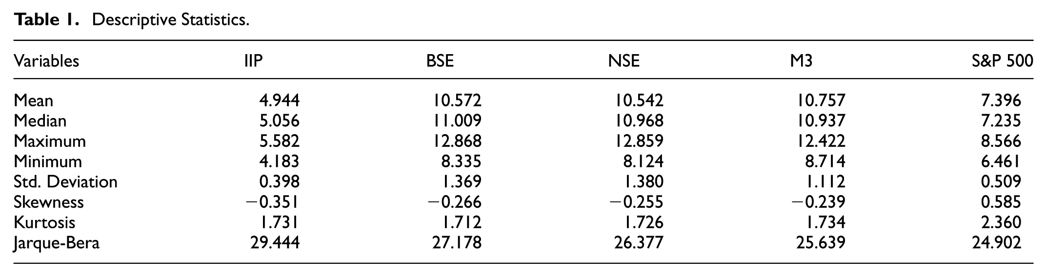
Negative skewness indicates that these variables experience sharper downturns than upturns. However, a positive S&P 500 indicates that the distribution had a longer right tail. Additionally, low kurtosis reflected smoother fluctuations, while the S&P 500 had relatively more outliers. The significant Jarque-Bera value indicates that the variables were not normally distributed.

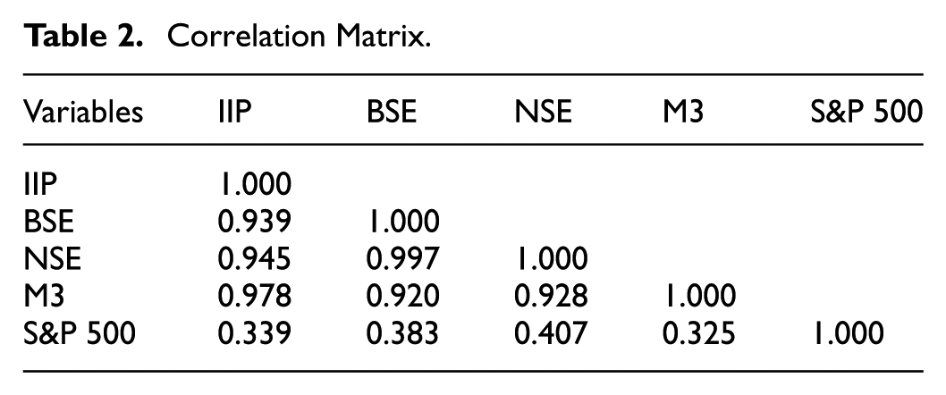
Correlation

Table 2 reports the results of correlations among the variables. The combined market capitalization of the BSE and NSE was highly correlated with IIP. As expected, M3 showed a strong positive correlation with IIP, while the global index S&P 500 had a moderate relationship with IIP, indicating some synchronization with the global market.

Table 2.

Correlation Matrix.

Variables	IIP	BSE	NSE	M3	S&P 500
IIP	1.000
BSE	0.939	1.000
NSE	0.945	0.997	1.000
M3	0.978	0.920	0.928	1.000
S&P 500	0.339	0.383	0.407	0.325	1.000

Unit Root Test

The Augmented Dickey-Fuller (ADF) and Phillips-Perron (PP) were used to check the stationarity of the variables. The results presented in Table 3 indicate that none of the variables were stationary at the level according to both the ADF and PP tests.

Table 3.

Unit Root Test Results.

Tests	Augmented Dickey-Fuller		Phillips-Perron
Variables	Level	1st Difference	Level	1st Difference
IIP	−1.384	−6.446***	−1.813	−69.836***
BSE	−0.250	−16.580***	−0.112	−16.599***
NSE	−0.288	−16.420***	−0.263	−16.506***
M3	−1.907	−1.782	−3.715	0.0043**
S&P 500	−0.181	−17.949***	−0.226	−18.002***

Note. ***, **, and * denotes significance at 1%, 5%, and 10% respectively.

However, IIP, BSE, NSE and S&P 500 became stationary after first differencing as per the ADF and PP test at the 1% level. M3 was found to be stationary at the first difference under the PP test. This implies that all the variables were integrated of order one, I(1).

Characteristics of Cycles

The cyclical components of the stock market (BSE and NSE), IIP, M3 and S&P 500 were derived using the Hodrick-Prescott filter and the lambda = 129,600. The characteristics captured the number of peaks, troughs, amplitude, the slope, and the largest cycle observed and also the co-movements among the variables.

Cyclical Characteristics of IIP

Figure 1 shows the cyclical fluctuations of IIP during the period. IIP experienced 7 peaks to peaks and 6 troughs to troughs, completing a full business cycle. These cycles resulted in 8 contractions and 7 expansions, respectively. The most significant downturn (trough to peak) occurred from 2018 to 2019, when the economic growth experienced contraction due to the outbreak of COVID-19, collapsing in 2020, and was followed by 2021 to 2022 with amplitudes of −0.3157 and −0.3504, respectively. This caused a sharp decline in the IIP index from 51.8 in March to 27.4 in April, marking the sharpest decline in Indian history (Varghese & Chandramana, 2022). While it was a short-lived collapse followed by a quick recovery, it could not be captured by the BB identification scheme. However, the IIP also showed different phases of expansion between 1999 to 2001 due to financial liberalization and the IT boom, with a growth of 6.8%. A slowdown was observed during the 2008 financial crisis due to a fall in exports, reducing the growth to 2.4%. Notably, the most prominent cycle (peak to peak) was observed between March 2007 and December 2009, with an amplitude of 0.090, aligning with the global financial crisis, and causing high fluctuations in industrial output.

Figure 1.

Cyclical component of the Index of Industrial Production (IIP).

Cyclical Characteristics and Co-movement of the Stock Market and IIP

BSE exhibited a complete cycle of 8 peaks and 7 troughs during the observed period, as presented in Figure 2. These cycles experienced 6 contractions and 5 expansions. Between 1998 and 2000, BSE saw a sharp increase with a trough-to-peak amplitude of 0.7594, lasting for 15 months. During this period, BSE Bolt expanded nationwide in 1997. Additionally, the BJP-led NDA won the 13th Lok Sabha election, and the Sensex crossed the 5,000 mark. This growth was followed by a significant decline in 2001, with an amplitude of −0.9454, due to the dot-com bubble burst (Modak et al., 2022). Notably, a significant expansion occurred in 2020-21, when the market turnover reached 10.45 lakh crore, and BSE recorded a high valuation, indicated by a high price-to-earnings ratio (Satyanarayanamma & Reddy, 2022). The largest cycle was observed between 2007 and 2009 with an amplitude of 0.4899, when the Sensex fell 1408 points, or 7.45%, due to the global financial crisis.

Figure 2.

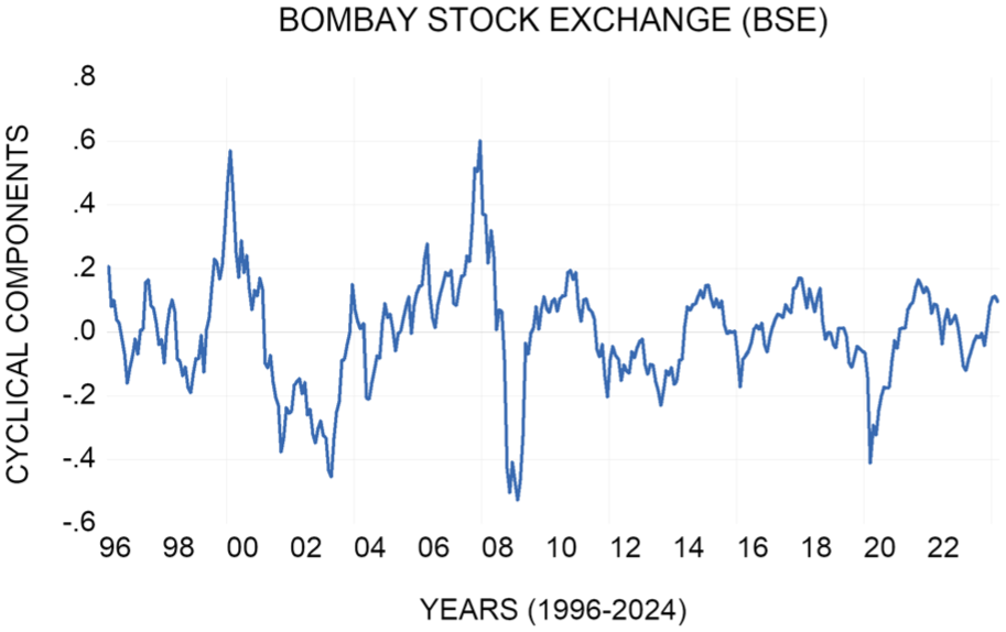
Cyclical component of the Bombay Stock Exchange (BSE).

NSE also completed a full cycle displayed in Figure 3, consisting of 7 peaks and 6 troughs, along with 6 contractions and 5 expansions. The period between 1998 and 2000 was a remarkable phase for NSE, as it experienced a significant upturn with an amplitude of 0.8954, lasting 15 months. This happened due to large investments by FIIs of US$2.34 billion. Market capitalization of NSE was 488,229 crores in April 1999, increasing to 1,020,426 crores in March 2020, almost recording a growth of 100%, followed by a contraction caused by the dot-com bubble burst, with an amplitude of −0.8927 from 2000 to 2001, lasting for 19 months (SEBI). A sharp downturn was observed during the period 2007 to 2010, due to the global financial crisis, extending over 29 months. The largest cycle for NSE, from peak to peak, occurred between February 2000 and December 2004, over 58 months, with an amplitude of 0.5390 due to the bubble burst in stock prices. Both indices were severely impacted from 2018 to 2020 due to lockdowns and global financial fluctuations.

Figure 3.

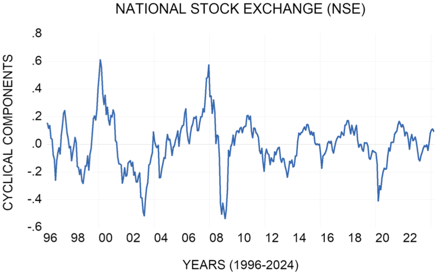
Cyclical component of the National Stock Exchange (NSE).

BSE displayed similar cyclical patterns with IIP, as shown in Figure 4, featuring several aligned expansions and contractions. The synchronization was particularly evident during the period of structural shocks. This indicates suggests a strong co-movement between the stock market and business cycles, suggesting pro-cyclical behavior, with the stock market leading real economic activity.

Figure 4.

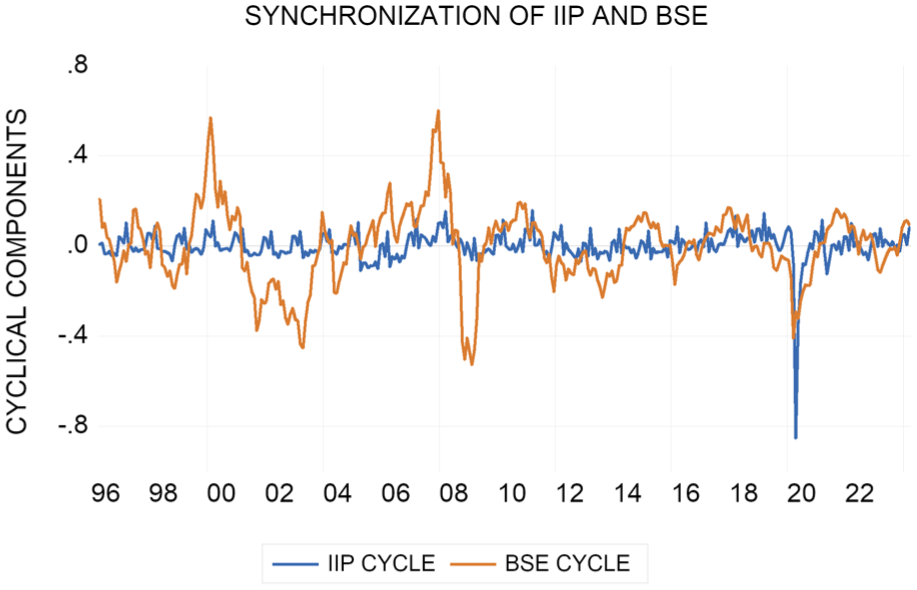
Synchronization of IIP and BSE cycles.

Similarly, NSE displayed a closely linked cyclical pattern with IIP, as shown in Figure 5. However, the stock market experienced more fluctuations, highlighting its higher sensitivity to shocks compared to economic growth.

Figure 5.

Synchronization of IIP and NSE cycles.

Cyclical Characteristics and Co-movement of M3 and IIP

Furthermore, M3 displayed 4 peak-to-peak and 3 trough-to-trough cycles, as presented in Figure 6. These cycles experienced 6 expansions and 7 contractions. During the period 2004 to 2005, M3 increased to 16.4% from 12.8% in the previous year. A significant upturn was observed between 2006 and 2008. Afterwards, it was affected by the 2008 financial crisis; however, the effect was not substantial, as it was seen in other variables. Its amplitude was −0.0344, reflecting temporary monetary tightening due to the outflow of foreign exchange. However, the RBI took necessary measures between October 2008 and April 2009 to increase liquidity. The repo rate and reverse repo rate were reduced to 4.75% and 3.25%, respectively (Mohanty, 2009). A significant downturn was observed from 2016 to 2017, with an amplitude of −0.0586, due to demonetization, where 89.6% of currency was eliminated from the economy, causing a temporary shortage of cash in the banks and ATMs. While the absolute level of M3 increased unexpectedly during the period of COVID-19 by 6.7%, an expansion occurred from 2020 to 2023.

Figure 6.

Cyclical component of Broad Money Supply (M3).

Additionally, M3 cycles exhibited similar movement with IIP cycles as illustrated in Figure 7, particularly during the period of financial crisis and the COVID-19 pandemic. However, outside this, the relationship appeared weaker. The magnitude of M3 fluctuations was smaller, as it is policy-driven and controlled by the RBI, resulting in low-level fluctuations.

Figure 7.

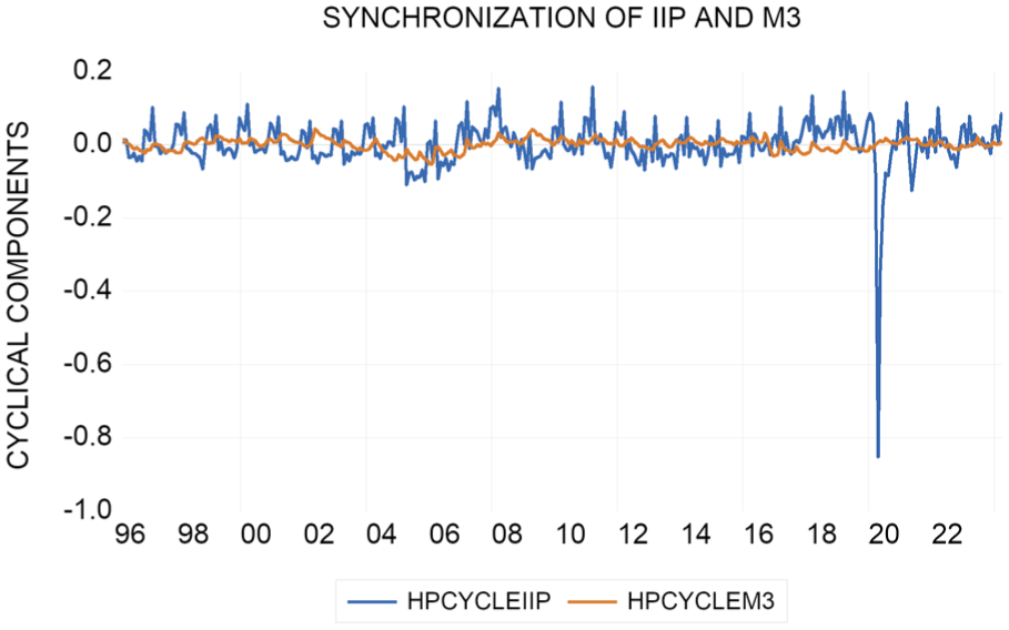
Synchronization of IIP and M3 cycles.

Cyclical Characteristics and Co-movement of S&P 500 and IIP

Lastly, the S&P 500 displayed 5 peak-to-peak cycles and 4 trough-to-trough cycles, as shown in Figure 8, reflecting fewer but more pronounced cycles. A total of 7 contractions and 8 expansions were observed. A major contraction occurred between 2007 and 2009 (peak to trough) due to the financial crisis, with an amplitude of −0.7222, lasting for 16 months. The demand for housing in the United States declined due to rising interest rates in 2006, which led to the depreciation of assets in the stock market. The S&P 500 experienced a pronounced decline during the crisis due to the interaction of various global factors (Nagy et al., 2024). During the COVID-19, stock prices fell sharply mainly in February and March, by at least 25%, but only for the first four months. The largest cycle was observed from 2006 to 2009 with an amplitude of 0.5195; its effects persisted for nearly 32 months.

Figure 8.

Cyclical component of S&P 500.

The synchronization graph presented in Figure 9 highlights that the S&P 500 and IIP appeared to be weakly correlated, with moderate co-movements during the financial crisis and COVID-19 period. Moreover, the S&P 500 exhibited stronger fluctuations, reflecting its sensitivity to worldwide investors’ sentiments. This implies that the global financial cycle does not influence the domestic business cycle.

Figure 9.

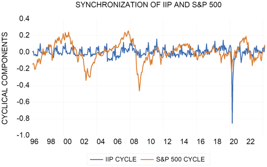
Synchronization of IIP and S&P 500 cycles.

Lead-Lag Relationship

The lead-lag relationship was employed to understand the direction of the cyclical interaction among the variables and to examine whether the market anticipates or follows real sector uncertainties.

Stock Market (BSE and NSE) and IIP

The lag column explains that BSE leads IIP, where the past values of BSE explain the current value of IIP, as presented in Table 4. Lead, on the other hand, indicates IIP leads BSE. The results revealed at lag 0 that both variables moved in the same direction, suggesting a contemporaneous relationship.

Table 4.

Lead-Lag Relationship Between BSE and IIP.

IIP, BSE (−i)		IIP, BSE (+i)
I	lag	i	lead
0	0.2613	0	0.2613
1	0.2986*	1	0.2244
2	0.2328	2	0.1802
3	0.2016	3	0.1248

Note. Lead-lag correlations were computed up to 36 lags. Only the first few meaningful coefficients were shown.

Denotes the peak coefficients with an absolute value > than 0.20.

BSE led IIP by approximately 1 month, with a highest coefficient of 0.2986 at lag 1. At lag 2 (0.2328) and 3 (0.2106), BSE continued to lead IIP, with the high positive coefficients. This suggests that capital market dynamics or shifts may predict economic activity by reflecting investors’ expectations in the short-run. However, the lead column showed the weak and insignificant correlations, confirming that IIP did not lead BSE. Similarly, in Table 5, same patterns were observed between NSE and IIP. NSE also led IIP by 1 month with a peak coefficient of 0.2902. However, the relationship weakened after 2 lags, indicating a short-lived impact. Overall, the stock market cycles influenced business cycles, but no meaningful effect of business cycles on the stock market cycles was observed.

Table 5.

Lead-Lag Relationship Between NSE and IIP.

IIP, NSE (−i)		IIP, NSE (+i)
I	lag	i	lead
0	0.2604	0	0.2604
1	0.2902*	1	0.2248
2	0.2281	2	0.1805
3	0.1978	3	0.1267

Note. Lead-lag correlations were computed up to 36 lags. Only the first few meaningful coefficients are shown.

Denotes the peak coefficients with an absolute value > than 0.20.

M3 and IIP

The lag and lead columns in Table 6 revealed a weak relationship between M3 and IIP. There was no strong or meaningful relationship observed between them; the value of the coefficient was less than the 0.20 threshold. The highest lag coefficient was at 9 lag (0.1696), and the lead exceeded the coefficient at 27 lag (0.1739), which means IIP slightly had a predictive power, but only after a long lag. However, the strength of the relationship remained weak. This could be due to the counter-cyclical nature of monetary policy.

Table 6.

Lead-Lag Relationship Between M3 and IIP.

IIP, M3 (−i)		IIP, M3 (+i)
I	lag	i	lead
0	−0.0282	0	−0.0282
1	−0.1081	1	0.0241
2	−0.0529	2	0.0673
3	−0.0488	3	0.1062

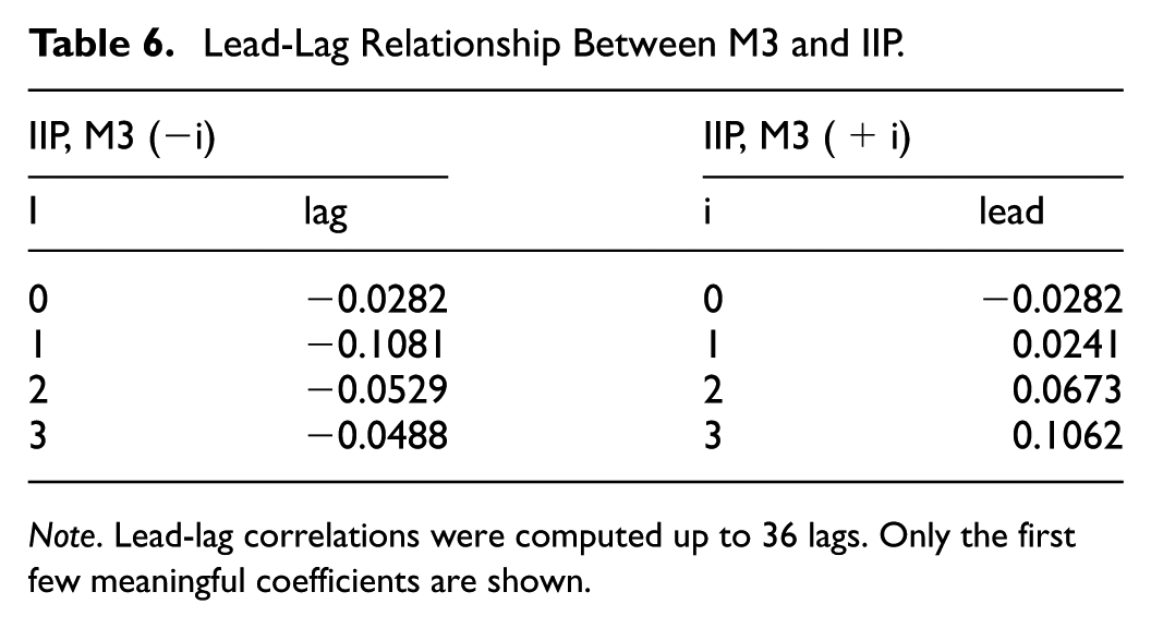
Note. Lead-lag correlations were computed up to 36 lags. Only the first few meaningful coefficients are shown.

S&P 500 and IIP

An interesting relationship was observed in Table 7 between the S&P 500 and IIP. The lag column showed no contemporaneous relationship observed, indicating no immediate influence of S&P movements on the IIP. However, the S&P 500 led IIP by 1 month. The peak coefficient was observed at lag 1 (0.2165); when S&P 500 moved, the IIP followed the same direction. Notably, the lead column revealed an inverse relationship between them, with the highest negative coefficient at lag 19 (−0.2318).

Table 7.

Lead-Lag Relationship Between S&P 500 and IIP.

IIP, S&P 500 (-i)		IIP, S&P 500 (+i)
I	lag	i	lead
0	0.1749	0	0.1749
1	0.2165*	1	0.1417
....	.....	....	.....
18	−0.0292	18	−0.2310
19	−0.0457	19	−0.2318*
20	−0.0381	20	−0.2300

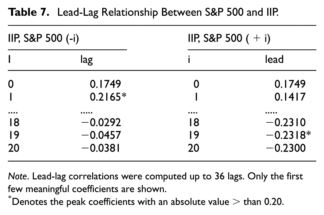
Note. Lead-lag correlations were computed up to 36 lags. Only the first few meaningful coefficients are shown.

Denotes the peak coefficients with an absolute value > than 0.20.

IIP negatively led the S&P 500 by the 19th month, and the negative impact lasted until the 20th period. Hence, the past increase in the IIP had a negative influence on the global financial market in the long-run. The findings align with the findings of (Goodrick & Sayama, 2024), who observed the lead-lag relationships that evolve depending on the economic conditions and structural shifts.

Granger Causality Test

Subsequently, a Granger causality test was performed, as presented in Table 8 on the cyclical values, to confirm the direction of the relationship among the variables using 12 lags.

Table 8.

Granger Causality Results.

Variables	F-statistics (p-value)	Direction of causality
BSE—IIP	2.76560 (0.0012)	Unidirectional causality from BSE to IIP cycles
IIP—BSE	0.67875 (0.7717)	Unidirectional causality from BSE to IIP cycles
NSE—IIP	2.72049 (0.0017)	Unidirectional causality from NSE to IIP cycles
IIP—NSE	0.64529 (0.8027)	Unidirectional causality from NSE to IIP cycles
M3—IIP	2.41801 (0.0053)	Bidirectional causality between M3 and IIP cycles
IIP—M3	2.31403 (0.0077)	Bidirectional causality between M3 and IIP cycles
S&P 500—IIP	3.60875 (5.E-05)	Unidirectional causality from S&P 500 to IIP
IIP—S&P 500	0.91443 (0.5327)	Unidirectional causality from S&P 500 to IIP

It was observed that BSE and NSE Granger caused IIP at the 5% significance level. However, no relationship was observed from IIP to BSE and NSE. This suggests a unidirectional relationship between the variables, indicating that past values of both the indices had some explanatory power for IIP in the short-run. Interestingly, these findings are consistent with both Keynesians’ and Monetarists’ views, indicating a bidirectional relationship between the IIP and M3. An expansionary money supply lowers the interest rates, which influence consumer spending and investments. Whereas, as suggested by Post-Keynesians, the money supply is endogenously determined by credit demand; as industrial production rises, the demand for credit increases, thereby increasing the money supply (Pollin, 1991).

Moreover, the S&P 500 Granger caused IIP, reflecting a unidirectional relationship. This implies that the global equity market has some predictive power in explaining domestic economic activity, while India’s economic activity has no explanatory power.

SVAR Analysis

The structural ordering of the SVAR was informed by the Granger causality test results. The findings indicated that BSE and NSE Granger caused IIP, while M3 exhibited a bidirectional relationship with IIP. Given this, IIP was reserved as the most endogenous variable, justifying the ordering. The results of SVAR further revealed the meaningful short- and long-run interdependencies among IIP, BSE, NSE, and M3, highlighting the dynamic interactions among business, financial, and monetary cycles.

Optimal Lag Length Criterion

Five criteria were used to determine the optimal lag length for the model: LR, FPE, AIC, SC and HQ. These criteria indicated that twelve lags were optimal, as suggested by the lowest SC, also identified by LR, as shown in Table 9. For monthly data, at least a year of lag is required to analyze the cyclical fluctuations of each variable.

Table 9.

VAR Lag length Selection Criteria.

Endogenous variables: BSE, NSE, M3 and IIP

Exogenous variable—C and S&P 500

LAG	Log L	LR	FPE	AIC	SC	HQ
0	2161.80	NA	1.98e-11	−13.2950	−14.7532	−13.2578
1	2810.42	1273.22	3.98e-13	−17.2001	−16.9201*	−17.0883*
2	2830.27	38.4751	3.89e-13*	−17.2239*	−16.7571	−17.0376
3	2838.90	16.5114	4.07e-13	−17.1784	−16.5249	−16.9176
4	2852.92	26.4801	4.12e-13	−17.1662	−16.3260	−16.8308
5	2864.09	20.8305	4.253-13	−17.1364	−16.1095	−16.7254
6	2872.44	15.3536	4.46e-13	−17.0891	−15.8755	−16.6047
7	2886.73	25.9280	4.51e-13	−17.0785	−15.6783	−16.5196
8	2902.16	27.6212	4.53e-14	−17.0750	−15.4880	−16.4416
9	2910.43	14.6035	4.75e-13	−17.0273	−15.2536	−16.3194
10	2920.67	17.8312	4.93e-13	−16.9918	−15.0314	−16.2093
11	2938.01	29.7547	4.90e-13	−17.0001	−4.8530	−16.1431
12	2982.38	75.0423*	4.12e-13	−17.1752	−14.8414	−16.2436

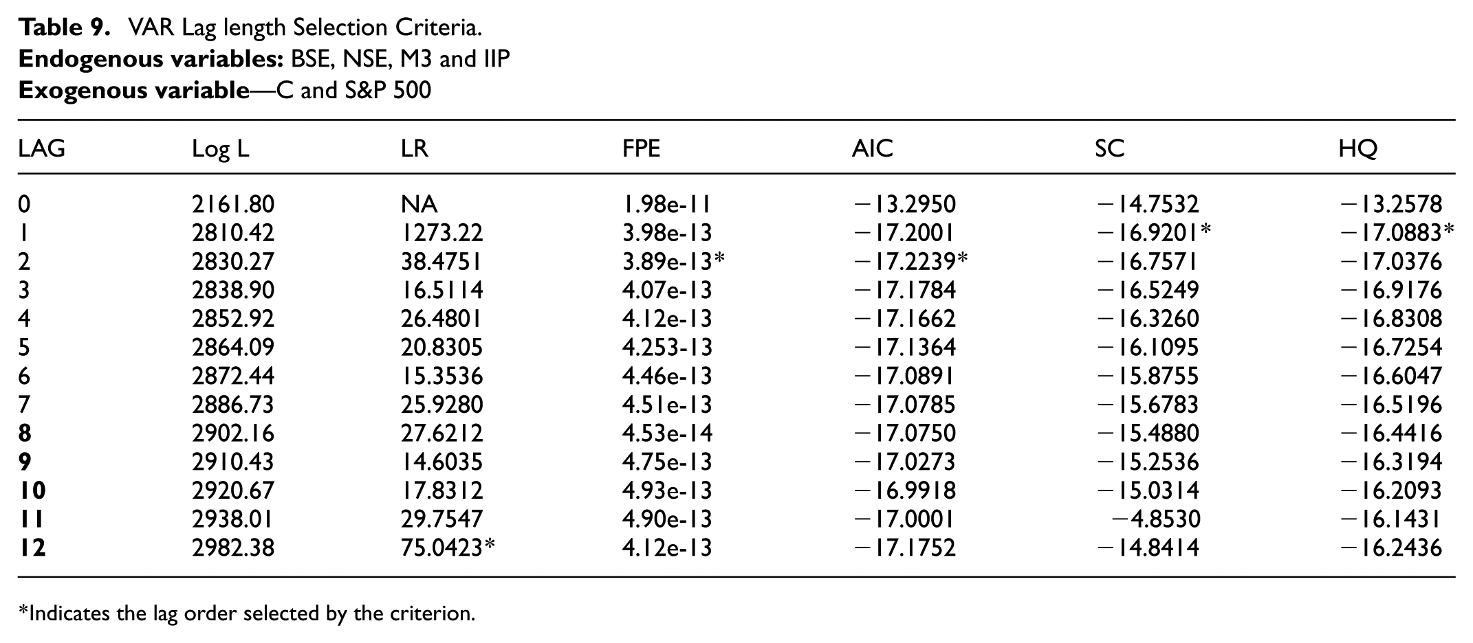
Indicates the lag order selected by the criterion.

Short-Run SVAR Estimates

The short-run SVAR (Structural Vector Autoregression) estimation aimed to capture the cyclical dynamics or short-term impacts of shocks on the variables. The model included five variables, where the S&P 500 was treated as an exogenous variable. This reflects the assumption that the U.S. market cannot be contemporaneously influenced by the Indian economic activity.

Estimated S-Matrix

Model: e = Su where E[uu’] = 1

Structural VAR is just identified

S [\begin{matrix} variables \\ BSE \\ NSE \\ M 3 \\ IIP \end{matrix}] {\begin{matrix} ε^{BS E_{t}} & ε^{NS E_{t}} & ε^{M 3_{t}} & ε^{II P_{t}} \\ 0.0661 * * * & 0 & 0 & 0 \\ 0.0644 * * * & 0.0161 * * * & 0 & 0 \\ - 0.0003 & 0.0002 & 0.0079 * * * & 0 \\ - 0.0005 & 0.0005 & - 0.0008 & 0.0567 * * * \end{matrix}}

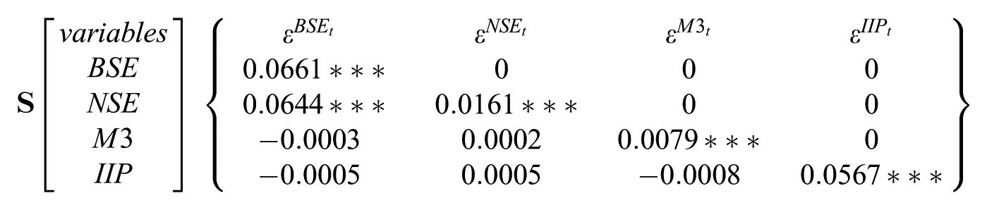
The model estimated the relationship between the variables during the period of fluctuations and how shocks to one variable affected the other in the short-run. BSE was assumed to be only affected by its own innovation, and not affected by the shock from the other variables in the model. The shocks to BSE were found to positively and significantly influence them. Additionally, BSE shocks influenced NSE, suggesting a close relationship between both indices. NSE also positively and substantially responded to its shocks. M3 shocks were not influenced by any other shocks except their structural shocks, suggesting no short-run linkages between stock market cycles and monetary policy. IIP was also self-driven and not influenced by shocks to other variables.

Long-Run SVAR Estimates

The long-run pattern matrix enabled the examination of the dynamics among the selected variables, showing how their relationship persists or evolves over an extended horizon.

Estimated F-Matrix

Model: e = Phi*Fu where E[uu’] = 1

Structural VAR is just identified

F [\begin{matrix} variables \\ BSE \\ NSE \\ M 3 \\ IIP \end{matrix}] {\begin{matrix} ε^{BS E_{t}} & ε^{NS E_{t}} & ε^{M 3_{t}} & ε^{II P_{t}} \\ 0.2685 * * * & 0 & 0 & 0 \\ 0.2199 * * * & 0.1575 * * * & 0 & 0 \\ - 0.0674 * * * & 0.1168 * * * & 0.0927 * * * & 0 \\ 0.0321 * * * & 0.0799 * * * & 0.0871 * * * & 0.1109 * * * \end{matrix}}

The long-run SVAR results revealed that shocks to BSE positively influenced themselves, with a coefficient of 0.2685, and statistically significant at the 1% level. The shocks to NSE had a positive influence on BSE, while NSE was positively influenced by its own structural shocks. A close relationship was observed between the NSE and BSE cycles, correlating with the findings of Bhinde and Shukla (2019). Additionally, Babu et al. (2023) confirmed homogeneous growth between BSE and NSE. Interestingly, M3 negatively responded to BSE shocks while positively responding to NSE shocks. The NSE is more technology-driven, reflecting greater optimism and higher demand for credit, as well as M3 growth (Geetha Devi & Gandikota, 2018). Previous literatures have also documented a positive relationship between the stock market and M3 in India (Sharma, 2018). Unlike all the other variables, it’s remained self-driven. While the long-run impact of BSE shocks on IIP remained modest, it was positive and significant, consistent with the findings of Dasgupta (2012). The shocks to NSE had a more pronounced effect on IIP, implying that both the stock markets contribute to economic growth. The shocks to M3 also confirmed a long-run relationship from liquidity to real growth. These findings align with the Monetarist approach, which believes that the money supply is an important driver of economic growth. Furthermore, IIP was also self-explanatory, positively influenced by their past performances.

Long-Run Impulse Response Function

Structural IRF traces the dynamic response of BSE to a one-unit innovation to each variable. Figure 10 reveals that BSE resulted in an immediate positive impact from most of the shocks in the short run, except for the IIP. Notably, BSE was primarily driven by its innovation up to the 8th period, suggesting the presence of a short-run relationship. Similarly, NSE shocks had a small positive influence. However, it declined gradually, confirming strong linkages in the short-run. While M3 shocks had a negative influence initially, they became flat afterwards, reflecting no persistent long-run influence, implying liquidity does not directly stimulate the capital market. IIP shocks had a negative short-run influence on BSE while positively influencing it in the long-run; however, the small coefficients indicated slow positive adjustment.

Figure 10.

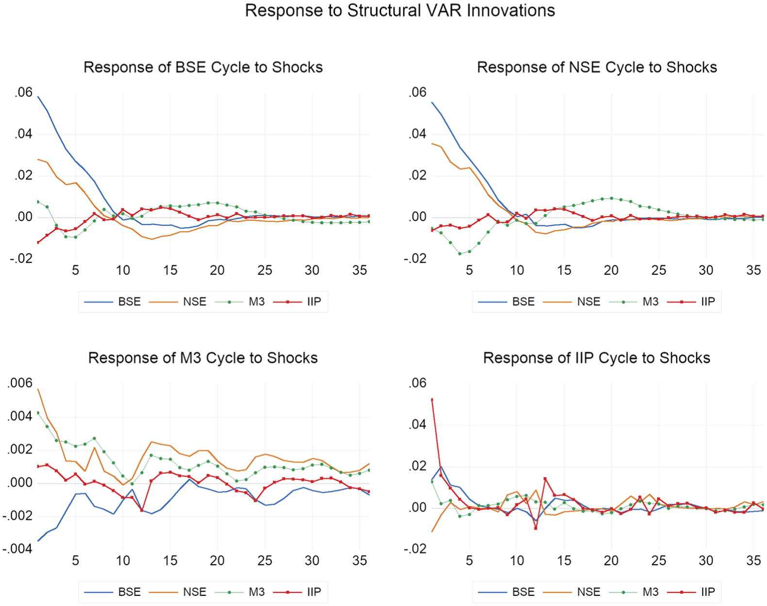
Impluse response function.

Similarly, the NSE exhibited a similar pattern to the BSE, with an initial positive response to the shocks in most of the variables, except IIP. It responded strongly to BSE shocks during the first 11 months, indicating a close relationship between them. While M3 had a negative impact on NSE until the 12th month, it was close to zero over the years. The results support the notion that broad money does not immediately stimulate equity market movements. Similarly, NSE was negatively influenced by IIP shocks and decreased by 0.0062 units, with a consistent negative effect until the 11th month. However, there were persistent long-run positive effects of these variable shocks on NSE, but they were moderate. Though we can say that innovation in real economic activity promotes growth in the equity market, with a time lag. This also suggests that NSE is more sensitive to shocks with stronger and longer impulse responses.

Further, M3 positively responded to its innovation over the years, implying monetary persistence. However, BSE shocks had a consistent negative influence on M3, indicating that fluctuations in the stock market may lead to inverse effects on M3, but it declined in the long-run. NSE shocks had a positive influence on M3 over the years. This implies liquidity creation boosts investors’ confidence, increasing the equity prices and growth. IIP shocks had a mild positive influence on M3, near zero, implying a lagged relationship between them. The findings imply that since M3 is policy-driven and controlled by the RBI, the effects on it are short-lived.

Additionally, the impulse response of IIP exhibited a mixed relationship over the forecast horizons. IIP positively responded to BSE shocks in the short-run with a strong positive coefficient, which diminished over time, implying that a sudden change or upturn in the stock market strengthens investor confidence and boosts economic growth in the short-run. Moreover, M3 shocks initially had a positive coefficient but later turned negative, implying M3 had a weak and inconsistent influence on IIP across both periods. However, NSE shocks initially had a negative influence on the growth, followed by a mild recovery. While IIP shocks had a predominantly positive and self-reinforcing influence on themselves, and a negative influence in some periods, this might be due to over-optimization of resources or inflationary pressure. The IRF of IIP indicates that real economic activity is influenced by both financial and liquidity markets.

Long-Run Variance Decomposition

The SVAR variance decomposition presented in Figure 11 illustrates the importance of an innovation or a shock in determining variations in the variables. BSE played a prominent role in explaining its forecast error, accounting for 77% in the first period, 17% by NSE, 1% by M3, and 3% by IIP shocks. BSE was largely explained by its fluctuation, stabilizing at approximately 71% in the long-run, suggesting the presence of self-reinforcing interactions in the economy. NSE also played an important role in explaining BSE. The contribution of NSE remained consistent and significant over the years, accounting for up to 21% in the long-run. While the role of M3 increased as the horizons expanded, the explanatory power remained moderate, reflecting that M3 operates through bank and credit channels, while the stock market responds to fluctuations immediately. Consequently, the relationship between the monetary and financial markets remained limited. IIP had a limited role in explaining BSE shocks, implying a mild influence of real market fluctuations on the BSE.

Figure 11.

Variance decomposition.

Similarly, NSE revealed that in the first year, 69% of the variance in forecast error was explained by BSE and 28% by NSE. The remaining variable had no explanatory power. However, in the fifth period, BSE mainly explained NSE; however, it declined to 64%, and NSE explained 29% of itself. The influence of NSE had progressed as the horizons expanded, implying a growing NSE market strength. Interestingly, the role of M3 was increased to 9%, reflecting a moderate role of liquidity transmission on financial markets, and IIP remained limited. The findings suggest a strong correlation among the stock market itself. The limited role of IIP suggests that market fluctuations are not primarily driven by economic activity.

Furthermore, M3 illustrated that in the first month, 19% of the variance in forecast error was explained by BSE, with M3 itself accounting for 28%, and the majority (50%) being explained by NSE. The results persisted over the long period, and NSE shocks dominated M3, followed by M3 and BSE. NSE remained the dominant variable in explaining M3. However, its contribution reduced marginally from 50 to 43% as the horizons expanded. The results suggest a significant integration of the capital market and monetary aggregates. The IIP shocks had a relatively low impact, increasing slowly from 1 to 4% in 36 months.

Lastly, the variance decomposition of IIP showed that during the first period, IIP had a major explanatory power of 84% in explaining its variance. IIP was primarily self-driven over the years, but its dominance declined with increased financial integration and the interplay among other variables. BSE accounted for a consistent and significant portion of IIP forecast variance, approximately 18%. This suggests BSE plays a prominent role in driving economic growth, but with a lag indicating a gradual transmission effect. The role of NSE and M3 increased in explaining IIP from 4% to 8% and 5% to 6% in the long-run, indicating a supporting indicator. However, the increasing role of variables highlights the existence of close relationships between the domestic financial markets and business cycles.

Robustness Test

To ensure the robustness of the findings, the lead-lag relationship was computed, as it captures the timings of co-movements. The cyclical series was divided into two equal parts, that is, Sample 1 (April 1996 to March 2010) and Sample 2 (April 2010 to March 2024), as reported in Table 10. The lead-lag correlation confirmed that BSE and NSE continued to lead IIP cycles by 1 to 3 months. In contrast, M3 exhibited a weak and inverse relationship in the aggregate and Sample 2 analysis, but showed a positive and moderate relationship in Sample 1, where IIP led M3, highest at lag 3. However, M3 did not show any meaningful impact on IIP. This suggests the impact of structural shocks on the money-output relationship. Possibly, during the contraction period, money supply is injected, causing an inverse relationship.

Table 10.

Robustness Test: Lead-Lag Relationship.

Variables	Aggregate sample	Sample 1	Sample 2
BSE-IIP	0.2986 (k = 1)	0.3119 (k = 1)	0.2992 (k = 1)
NSE-IIP	0.2902 (k = 1)	0.3022 (k = 1)	0.3022 (k = 1)
M3-IIP	Negative/Weak	0.3028 (k = 3), IIP-M3	Negative/Weak
S&P 500-IIP	0.2165 (k = 1)	0.2662 (k = 1)	0.2140 (k = 1)

Note. K denotes the number of months at which the coefficients reach at their peak.

Overall, the robustness test results align with the aggregate results, emphasizing the significant role of stock market cycles in influencing business cycles and predicting economic downturns. While the M3 and IIP relationship is regime-dependent.

Discussions and Policy Implications

The study provides updated findings on the dynamics between the stock market and macroeconomic indicators over the past 28 years, with the combination of various econometric methods, like lead-lag relationship, Granger causality, impulse response function, and variance decomposition. The last phase of financial and business cycles outlined the recent shocks, including demonetization and COVID-19. The most influential shocks experienced by equity markets were the global financial crisis and COVID-19, both confirmed by turning point analysis. IIP exhibited a cycle with a typical duration of 36 months, aligning with the findings of Avyukt (2018).

The synchronization of HP filter graphs confirmed the pro-cyclicality of stock market indices (BSE and NSE) with IIP. Additionally, the lead-lag relationship confirmed that financial cycles lead business cycles by approximately 1 to 3 months. While long-run SVAR reinforced that the capital market is a leading indicator, it reflects real-time information and investors’ sentiments. Therefore, SEBI and RBI should monitor financial volatility and trends more closely and manage financial activities. In line with Topcu and Gulal (2020), particularly during times of crisis, it becomes imperative to intervene promptly and adopt an extensive policy to boost economic output.

The primary role of monetary policy is to stabilize prices in the long-run. The Reserve Bank of India, through its inflation targeting framework (2% or 4%), aims to manage liquidity and reduce uncertainty. The observed long-run and bidirectional relationship between monetary policy and economic growth highlights its lagged effects, which have been confirmed by the monetary transmission mechanism. The RBI should sustain enough liquidity to support industrial growth, particularly during the crisis period. However, the M3 was less volatile and exhibited mild close movements with IIP; its expansion and contraction can have a significant influence on long-term growth, particularly during times of shocks and crises.

Regarding global dynamics, the cyclical co-movement revealed a weak or no relationship between the S&P 500 and IIP. However, only in the crisis periods, the global financial crisis and COVID-19, both variables showed a co-movement. This suggests that India, during crises depends on the global market, which makes it imperative to build foreign exchange reserves, enhance financial regulation, and achieve self-sufficiency.

Previous studies like Adam and Merkel (2019), Jawadi et al. (2022) posit that business cycle fluctuations anticipate stock market uncertainties in developed countries like the United States. Moreover, most existing studies found a bidirectional link between financial cycles and business cycles. This study differentiates itself by using monthly data from April 1996 to March 2024 and provides updated evidence on how these relationships have evolved over the years. The findings highlight the consistent positive impact of the stock market on leading IIP cycles, even during the major structural shocks. Further, an important contribution of the study lies in demonstrating that such relationships are not stable across all the samples. The money output interaction changed during the period April 1996 to March 2010, where IIP led M3. This implies that during this period, the monetary aggregate adjusted to the needs of the real economy. This highlights the importance of sub-sample analysis to gain a comprehensive understanding of how structural shocks reshape the relationship among the variables.

Conclusion

The dynamic nature of the financial market highlights its sensitivity to booms and busts. The financial crisis of 2008 and the recent COVID-19 pandemic have made it imperative to study the cyclical relationship between the Indian stock market (BSE and NSE), monetary policy (M3), and real economic activity (IIP). This study employed high-frequency monthly data from April 1996 to March 2023. It used the HP filter to extract the cyclical components and the BB algorithm to identify the turning points. The stock market indices exhibited more frequent cyclical fluctuations, closely following one another and displaying similar peaks and troughs. The strong co-movements between the two exchanges and IIP during the dot-com bubble, financial crisis, and COVID-19 suggested a close relationship among them, with the stock market appearing to be more volatile than the business market. Particularly post-2003, the indicators exhibited strong co-movement, indicating a procyclical relationship. The findings support the hypothesis that fluctuations in financial markets lead to business cycles, while M3 exhibited minimal fluctuations but showed visible co-movements with IIP cycles during the time of economic shocks. This aligns with M3 being less vulnerable to short-term economic shifts. However, the S&P 500 and IIP appeared to be procyclical, moving in the same direction only during the financial crisis and the COVID-19 pandemic. After this, their relationship weakened, reflecting the dominance of domestic factors in driving economic growth.

The lead-lag relationship revealed that both BSE and NSE led IIP, and financial markets anticipate turning points in business cycles by up to 3 months, peaking at lag 1. These results were also supported by the Granger causality test, which showed a unidirectional relationship from financial markets to the business markets. In contrast, while M3 and IIP exhibited a limited lead-lag relationship, the Granger test confirmed a bidirectional relationship between them. Furthermore, S&P led IIP by 1 month, indicating short-run global influence, followed by a negative influence of IIP on S&P with a longer lag of 20 months.

The structural dynamics captured by SVAR revealed the significant short-run relationship between the exchanges, while M3 and IIP predominantly influenced themselves. The long-run SVAR reported distinct results, however, confirming the persistent long-run relationship between BSE and NSE, with both sharing close movements and strong linkages. The contrasting impact of BSE and NSE shocks on M3 reflected the structural and behavioral differences between the two markets. Additionally, IIP positively responded to BSE, NSE, and M3 shocks. This suggests a close relationship between the stock index, money market, and real output. Moreover, the IIP growth contributed positively to long-term economic expansion. The variance decomposition indicated that the explanatory power of BSE, NSE, and M3 increased gradually over the years, indicating close movements and supporting the long-run relationship among them. Additionally, upturns in the capital market boost investor confidence, and demand for liquidity increases, reflecting the positive response of M3 to the fluctuations in the capital market. To ensure the stability of the findings, the robustness test was performed, and the sample was divided into two sub-samples (1996–2010 and 2010–2024). The stock market relationship remained consistent, confirming its predictive role. While the M3 and IIP relationship varied, reflecting its sensitivity to shocks.

Fianlly, this study is based on the HP filter technique, which smooths out the fluctuations, due to which the estimated coefficients may appear smaller. For future studies, methods like wavelet analysis and Hamilton can be used for a better understanding of this complex relationship. Additionally, a Principal Component Analysis (PCA) can be conducted to combine different stock indices to reduce the problem of multicollinearity and dimensionality. Further, the study can be extended to sectoral analysis to explore how fluctuations in monetary and financial markets affect sectoral activities. A panel study can be conducted across emerging economies and advanced economies to compare how strongly financial markets influence real economic output.

Footnotes

Acknowledgements

The author received no support for this research.

ORCID iDs

Ridhima Garg

Ash Narayan Sah

Ethical Considerations

There was no human or animal participation in this article, and no informed consent was required.

Author Contributions

RG was responsible for conceptualization, data collection, and formal analysis. RG also developed the methodology, conducted the empirical investigation, interpreted the results and prepared the original draft. AS provided project administration, overall supervision and contributed to the review and editing.

Funding

The authors received no financial support for the research, authorship, and/or publication of this article.

Declaration of Conflicting Interests

The authors declared no potential conflicts of interest with respect to the research, authorship, and/or publication of this article.

Data Availability Statement

The data that support the findings of this study are available from the corresponding author upon reasonable request.

References

Adam

Merkel

(2019). Stock price cycles and business cycles (European Central Bank Working Paper Series).

Ahmad

Sehgal

(2017). Business cycle and financial cycle interdependence and the rising role of China in SAARC. Journal of Quantitative Economics, 16(3), 185–225. https://doi.org/10.1007/s40953-017-0086-3

Amisano

Giannini

(1997). Topics in structural VAR econometrics. Springer-Verlag.

Aravalath

L. M.

(2020). Do financial cycles cause business cycles in India? Evidence from wavelet-based causality analysis. Journal of Public Affairs, 22(2), e2410. https://doi.org/10.1002/pa.2410

Atje

Jovanovic

(1993). Stock markets and development. European Economic Review, 37(2), 632–640. https://doi.org/10.1016/0014-2921(93)90053-D

Avyukt

(2018). Lead-lag relationship between credit and output cycles: Case of India and US. National Council of Applied Economic Research (NCAER) (Working Paper No. 116).

Babu

B. H.

Madhu

L. V.

Raghuveer

Sridhar

K. V.

(2023). A study on growth of Indian stock market: A comparative analysis between BSE Sensex and NSE Nifty. European Economic Letters, 13(5), 1823–1828.

Backus

D. K.

Patrick

J. K.

(1992). International evidence on the historical properties of business cycles. The American Economic Review, 82(4), 864–888.

Banerjee

Basu

Ghate

(2020). A monetary business cycle model for India. Economic Inquiry, Western Economic Association International, 58(3), 1362–1386.

10.

Baxter

King

R. G.

(1999). Measuring business cycles: Approximate band-pass filters for economic time series. The Review of Economics and Statistics, 81(4), 575–593.

11.

Behera

Sharma

(2022). Characterizing India’s Financial Cycle. Journal of Emerging Market Finance, 21(2), 152–183. https://doi.org/10.1177/097265272210777.

12.

Bhinde

Shukla

A. K.

(2019). NIFTY and SENSEX: A study of association between Indian Stock Markets. CNR’s International Journal of Social and Scientific Research, 50–54. https://doi.org/10.13140/RG.2.2.11286.32328

13.

Bhullar

P. S.

(2017). An empirical analysis of relationship between stock market development and economic growth: The Indian context. International Journal of Economic Research, 14(15), 523–536.

14.

Borio

(2012). The financial cycle and macroeconomics: What have we learnt? (BIS Working Paper). https://doi.org/10.1016/j.jbankfin.2013.07.031

15.

Bry

Boschan

(1971). Programmed selection of cyclical turning points. Cyclical Analysis of Time Series: Selected Procedures and Computer Programs (pp. 7–63), NBER.

16.

Burns

A. F.

Mitchell

W. C.

(1946). Working plans. In Measuring Business Cycles, (pp. 3–22). NBER.

17.

Chitre

V.S.

(2001). Indicators of business recessions and revivals in India: 1951-1982. Indian Economic Review, 36(1), 79–105. https://papers.ssrn.com/sol3/papers.cfm?abstract_id=329482

18.

Chauvet

(2001). Stock market fluctuations and the business cycle. Journal of Economic and Social Measurement, 25, 235–258. https://doi.org/10.2139/ssrn.283793

19.

Christiano

L. J.

Fitzgerald

T. J.

(1999). The band pass filter (NBER Working Paper 7257).

20.

Claessens

Ayhan

M. K.

Terrones

M. E.

(2011). How do business and financial cycles interact? (IMF Working Paper).

21.

Chikwira

Mohammed

J. I.

(2023). The impact of the stock market on liquidity and economic growth: Evidence of volatile market. Economies, MDPI, 11(6), 1–19. https://doi.org/10.3390/economies1106015

22.

Conrad

C. A.

(2021). The effects of money supply and interest rates on stock prices, evidence from two behavioral experiments. Applied Economics and Finance, 8(2), 33–34. https://doi.org/10.11114/aef.v8i2.5173

23.

Dasgupta

(2012). Long-run and short-run relationships between BSE SENSEX and macroeconomic variables. International Research Journal of Finance and Economics, 95, 135–150.

24.

Demir

(2025). The role of stock markets in economic growth: Empirical evidence from panel data analysis (Working Paper No. 7). WFE Research.

25.

Fischer

Merton

R. C.

(1984). Macroeconomics and finance: The role of the stock market. Carnegie—Rochester Conference on Public Policy. Cambridge, MA 02138, National Bureau of Economic Research.

26.

Geetha Devi

K. V.

Gandikota

(2018). The effect of microeconomic determinants on the Indian stock market. International Journal of Management, Technology, and Engineering, 8(5), 500–515.

27.

Ghate

Pandey

Patnaik

(2012). Has India emerged? Business cycle stylized facts from a transitioning economy. SPF Financial and Monetary Policy Reform. Indian Council for Research on International Economic Relations. https://doi.org/10.1016/j.strueco.2012.08.006

28.

Ghosh

Chhaochhoria

(2020). Stock market performance and economic growth: A causal relation. Journal of Business and Management, 22(7), 9–21. https://doi.org/10.9790/487X-2207070921

29.

Goldsmith

(1969). Financial structure and development. Yale University Press.

30.

Goodrick

Sayama

(2024). Modeling and analysis of the lead-lag network of economic indicators. Data Science and Security, 213–226. https://doi.org/10.1007/978-981-97-0975-5_19

31.

Goyal

Kumar

(2018). Money and business cycle: Evidence from India. Indira Gandhi Institute of Development Research, Mumbai Working Papers 2018-020. https://www.researchgate.net/publication/328267639_Money_and_business_cycle_Evidence_from_India

32.

Hodrick

Prescott

(1981). Post–war U.S. business cycles: An empirical investigation. Journal of Money, Credit, and Banking (1997), 29(1), 1–16. https://doi.org/10.2307/2953682

33.

Hoque

M. E.

Yakob

N. A.

Kruse

(2017). Revisiting stock market development and economic growth nexus: The moderating role of foreign capital inflows and exchange rates. Cogent Economics & Finance, 5(1), 1329975–132. https://doi.org/10.1080/23322039.2017.1329975

34.

Jawadi

Ameur

H. B.

Bigou

Flageollet

(2022). Does the real business cycle help forecast the financial cycle? Computational Economics, 60, 1529–1546. https://doi.org/10.1007/s10614-021-10193-8

35.

Johansen

(1995). Likelihood-based inference in cointegrated vector autoregressive models. Oxford University Press.

36.

Johnson

T. E.

(1983). Investment principles. In Business & Economics. Prentice-Hall.

37.

Karagol

Doazan

(2021). Interaction between business and financial cycles: Evidence from Turkey. Eastern Journal of European Studies, 12, 123–150. https://doi.org/10.47743/ejes-2021-0207

38.

Keswani

Puri

Jha

(2024). Relationship among macroeconomic factors and stock prices: A cointegration approach from the Indian stock market. Cogent Economics & Finance, 12(1), 2355017. https://doi.org/10.1080/23322039.2024.2355017

39.

King

R. G.

Levine

(1993). King, R. G., & Levine, R. (1993a). Finance and growth: Schumpeter might be right. The Quarterly Journal of Economics, 108(3), 717–737. https://doi.org/10.2307/2118406

40.

Kirankabes

M. C.

Basarir

(2012). Stock Market development and economic growth in developing countries: An empirical analysis for Turkey. International Research Journal of Finance and Economics, 87, 136–146.

41.

Kumar

Prakash

(2022). Behaviour of credit, investment, and business cycles: The Indian experience. Reserve Bank of India Occasional Papers, 43(1), 119.

42.

Levine

Zervos

(1998). Stock markets, banks, and economic growth. American Economic Review, 88(3), 537–558. http://www.jstor.org/stable/116848

43.

Lutkepohl

(2005). New introduction to multiple time series analysis. Springer-Verlag.

44.

Lutkepohl

Kratzig

(2004). Applied time series econometrics. Cambridge University.

45.

Mahajan

D. D.

(2023). Importance of the stock market for the Indian Economy. IIBS. https://www.iibs.edu.in/news/importance-of-stock-market-for-indian-economy-997

46.

Management

RBC Asset.

(2009). Understanding the economic and stock market cycles. RBC Asset Management. http://funds.rbcgam.com/pdf/Understanding_Economic.pdf

47.

Mandal

Bhattacharjee

(2012). The Indian Stock Market and the Great Recession. Theoretical and Applied Economics, 19(3), 59–76. https://store.ectap.ro/articole/698.pdf

48.

Mankiw

N. G.

(1989). Real business cycles: A new Keynesian perspective. Journal of Economic Perspectives, 3(3), 79–90. http://www.nber.org/papers/w2882.pdf

49.

McKinnon

R. I.

(1973). Money and capital in economic development. The Brookings Institution.

50.

Meshram

Sarang

Jadhav

(2020). A study on trends and operations of Indian stock exchanges. Proceedings of Online National Level Conference on Innovative Business Strategies to Cope with the Present Era of Globalization. Pune, Maharashtra: A Multidisciplinary Peer-Reviewed Journal. https://ssrn.com/abstract=4496116

51.

Misra

(2018). An investigation of the macroeconomic factors affecting the Indian Stock Market. Australasian Accounting Business and Finance Journal, 12(2), 71–86. https://doi.org/10.14453/aabfj.v12i2.5

52.

Modak

Kant

Sahu

R. P.

Sethuraman

(2022). India at 75: 20 milestones for Indian markets between 1995 and 2002. Business Standard.

53.

Mohanty

(2009). Global financial crisis and monetary policy response in India. 3rd Indian Council for Research on International Economic Relations-Internationale Weiterbildung und Entwicklung. BIS Review, 10.

54.

Mohanty

Singh

Jain

(2003). Business cycles and leading indicators of industrial activity in India. MPRA Paper 12149. RePEc.

55.

Monahov

(2023). HPFilter: An R implementation of the one- and two-sided Hodrick-Prescott Filter. SSRN Electronic Journal, 4387670.

56.

Nagy

Katarina

Kovalova

Macura

(2024). Drivers of S&P 500’s profitability: Implications for investment strategy and risk management. Economies, 12(4), 77. https://doi.org/10.3390/economies12040077

57.

Pal

(2014). Financial policy of India—Theory & evidence from co-integration. H.R. Journal of Management, Forthcoming, 5(6), 96–103.

58.

Palamalai

Prakasam

(2014). Stock market development and economic growth in India: An empirical analysis. International Journal of Finance & Banking Studies, 3(3), 30–46. https://ssrn.com/abstract=2556144.

59.

Pandey

Shettigar

(2017). Relationship between monetary policy and industrial production in India. In Current Issues in Economics and Finance (pp. 37–52). Springer Nature. https://doi.org/10.1007/978-981-10-5810-3_3

60.

Paramanik

Bhandari

Kamaiah

(2021). Financial cycle, business cycle, and policy uncertainty in India: An empirical investigation. Bulletin of Economic Research, 74(3), 825–837. https://doi.org/10.1111/boer.12320

61.

Paramati

S. R.

Gupta

(2011). An empirical analysis of stock market performance and economic growth: evidence from India. International Research Journal of Finance and Economics, 73, 144–160. http://dx.doi.org/10.2139/ssrn.2335996

62.

Patrick

(1966). Financial development and economic growth in underdeveloped countries. Economic Development and Cultural Change, 14, 174–189. http://dx.doi.org/10.1086/450153

63.

Pollin

(1991). Two theories of money supply endogeneity: Some empirical evidence. Journal of Post Keynesian Economics, 13(3), 366–396. https://doi.org/10.1080/01603477.1991.11489855

64.

Prudente de Alcântara e Silva

Giorno

(2025). Business cycles, stock market and monetary policy in Brazil. Brazilian Review of Finance, 23(1), e202501. https://doi.org/10.12660/rbfin.v23n1.2025.92566

65.

Qamruzzaman

Wei

(2018). Financial innovation, stock market development, and economic growth: An application of the ARDL model. International Journal of Financial Studies, 6(3), 69. https://doi.org/10.3390/ijfs6030069

66.

(2024). A Review about the business cycle and the stock market. Advances in Economics, Management, and Political Sciences, 124(1), 234–238. https://doi.org/10.54254/2754-1169/2024.17720

67.

Ramchandraiah

(2024). An analysis of the Stock Market’s impact on economic growth: Insights from an Indian context. International Journal for Multidisciplinary Research, 6(5), 413–418.

68.

Ravn

Uhlig

(2002). On adjusting the Hodrick-Prescott filter for the frequency of observations. The Review of Economics and Statistics, 84(2), 371–376. https://doi.org/10.1162/003465302317411604

69.

Robinson

(1952). The generalisation of the general theory, in the rate of interest, and other essays. Macmillan.

70.

Rünstler

(2016). How distinct are financial cycles from business cycles? European Central Bank. https://www.ecb.europa.eu//pub/economic-research/r…html/rb160831.en.pdf

71.

Sanvi

D. A.

Matheron

(2005). Interactions between business cycles, financial cycles, and monetary policy: Stylized facts. BIS Papers, 22, 273–298. Investigating the relationship between the financial and real economy

72.

Satyanarayanamma

Reddy

K. V. R.

(2022). Growth and development of Bombay stock exchange in India: An empirical study. International Journal of Science and Research (IJSR), 11(1), 1173–1177. https://doi.org/https://www.doi.org/10.21275/SR22121180104

73.

Schrank

(2024). The impact of a crisis on monetary policy’s influence on financial markets: Evidence from the COVID-19 pandemic. Cogent Economics & Finance, 12(1), 2322874. https://doi.org/10.1080/23322039.2024.2322874

74.

Schumpeter

(1912). The theory of economic development. Oxford University Press.

75.

Sharma

P. C.

(2018). A study on affiliation between the indian stock market and macroeconomic variables. MUDRA Journal of Finance and Accounting, 5(01), 117–129. https://doi.org/10.17492/mudra.v5i01.13040

76.

Shankar

Dubey

(2021). Indian stock market during COVID-19 pandemic: Vulnerable or resilient?—Sector analysis. Organizations and Markets in Emerging Economies, 12(1), 131–159. https://doi.org/https://doi.org/10.15388/omee.2021.12.51

77.

Sultana

Sharma

Akheel

(2021). Stock market and economic growth: A study in Indian perspective. Empirical Economics Letters, 20(11), 1881–1890.

78.

Surya

(2024). India’s post-COVID growth: A mixed recovery. NewsClick.

79.

Tomar

K. S.

Kesharwani

(2021). Asymmetric effect of monetary policy on Indian stock market sectors: Do monetary policy stimulus transpire the same effect on all sectors? Cogent Economics & Finance, 10(1), 1–19. https://doi.org/10.1080/23322039.2021.1999058

80.

Topcu

Gulal

O. S.

(2020). The impact of COVID-19 on emerging stock markets. Finance Research Letters, 36, 101691.

81.

Varghese

J. M.

Chandramana

S. B.

(2022). Impact of Covid-19 on manufacturing sector in India. International Journal of Advanced Technology in Engineering and Science, 10(1), 35–41.

82.

Vatsa

Basent

H. C.

Mixon

F. G.

Upadhyaya

K. P.

(2024). Stock market cycles and macroeconomic dynamics. International Advances in Economic Research, 30, 255–278.

83.

Vatsa

P. B.

(2024). Stock markets, cycles and macroeconomic dynamics. International Advances in Economic Research, 30, 255–278. https://doi.org/10.1007/s11294-024-09901-5

84.

Vinayaranjan

Narasimha

R. V.

Sravani

(2022). GDP impact on market capitalization—An analysis of BSE. Journal of Rural Development, 57, 37–40.

85.

Yong

Zhang

(2016). Financial cycle, business cycle and monetary policy: Evidence from four major economies. International Journal of Finance and Economics, 21(4), 502–527. https://doi.org/10.1002/ijfe.1566

86.

Yan

Huang

(2020). Financial cycle and business cycle: An empirical analysis based on the data from the U.S. Economic Modelling, 93, 693–701. https://doi.org/10.1016/j.econmod.2020.01.018

Business and Stock Market Cycle Dynamics in India: A Monthly Analysis Using Turning Point and SVAR

Abstract

Plain Language Summary

Keywords

Introduction

Literature Review

Theoretical Framework

Supply-Leading and Demand-Following Hypotheses

Stage of Development Theory

Financial Liberalization Theory

Empirical Literature Review

Data and Variables

Methodology

Hodrick-Prescott Filter

Cross-Correlation (Lead and Lag Relationship)

Structural Vector Autoregression

Vector Autoregression Framework

Structural Vector Autoregressive Model

Structural Impulse Response Function and Variance Decomposition

Structural VAR Estimates on the Short-Run Pattern Matrix

Empirical Evidence

Descriptive Statistics

Correlation

Unit Root Test

Characteristics of Cycles

Cyclical Characteristics of IIP

Cyclical Characteristics and Co-movement of the Stock Market and IIP

Cyclical Characteristics and Co-movement of M3 and IIP

Cyclical Characteristics and Co-movement of S&P 500 and IIP

Lead-Lag Relationship

Stock Market (BSE and NSE) and IIP

M3 and IIP

S&P 500 and IIP

Granger Causality Test

SVAR Analysis

Optimal Lag Length Criterion

Short-Run SVAR Estimates

Estimated S-Matrix

Long-Run SVAR Estimates

Estimated F-Matrix

Long-Run Impulse Response Function

Long-Run Variance Decomposition

Robustness Test

Discussions and Policy Implications

Conclusion

Footnotes

Acknowledgements

ORCID iDs

Ethical Considerations

Author Contributions

Funding

Declaration of Conflicting Interests

Data Availability Statement

References