Sage Journals: Discover world-class research

Abstract

The objective of this paper is to examine the effect of government spending volatility on economic growth in an oil producing country—Saudi Arabia. The Hodrick–Prescott (HP) filtering approach was applied to decompose the data series into cyclical and trend components. The ordinary least squares, and nonlinear autoregressive distributed lag were also used, and the results confirm the negative effect of government spending volatility on real GDP growth in an oil-based economy. Moreover, the estimated coefficients of the nonlinear ARDL models indicate that changes in government spending have a significant short run and long run impact on real GDP growth, and real GDP growth responds asymmetrically to movements in government spending. Moreover, the more trade openness and credit fluctuate, the more volatile real economic growth is. Although the magnitude of government spending volatility is acceptable, the result proves that the exclusion of oil-based economies from the test of government spending volatility was inappropriate and unjustified. These results suggest that controlling the sources of instability in real GDP growth depends on the external sector and domestic credit. However, the successes of other countries should be presented and studied in order to choose appropriate policies that mitigate public spending volatility and contribute to sustainable economic growth.

Keywords

government expenditure volatility NARDL OLS HP filtering

Introduction

Oil-producing countries such as Saudi Arabia have been cynically described as having enough oil to create problems, but not enough to solve them (Gelb, 1981, p. 1). While oil revenues are seen as a blessing, their wide fluctuations can be a curse. Nevertheless, oil revenues dominate all sources of revenue in the kingdom that are controlled and managed by the government. Oil and gas revenues account for a significant portion of the national budget. In 1970, for example, the share of oil as a source of revenue reached 90% of total government revenue. In 1974, however, oil revenues accounted for about 94% of total revenues. Drawing on Norway’s experience, van Ingen et al. (2014) suggested that oil-producing countries should adopt a prudent fiscal rule to limit consumption to the flow of revenues from invested and accumulated assets to contain the volatility of their economies.

To what extent can fiscal policy affect real economic growth? Stounaras (2010) summarizes the viewpoints of various schools of economic thought in economics regarding fiscal policy and its role in determining economic growth. Fiscal policy affects economic growth during transitions, as is the case with exogenously induced technological progress and population growth. From a neoclassical perspective, however, variations in tax systems, government spending, and government debt are influential determinants of economic growth but not of actual output. Similarly, Keynesians using different models have suggested that macroeconomic policies play a major role in the observed differences across growth models. Therefore, output volatility can have a considerable negative effect on social welfare (Turan & Iyidogan, 2017). This strand of the literature is consistent with Ramey and Ramey (1995), Kim and Nelson (1999), and Badinger (2008).

Studies generally almost agree that there exists a negative relation between the size of state and economic growth. Accordingly, a 10% increase in tax revenues or government spending as a share of gross domestic product (GDP) leads to a negative impact on real growth of 0.5 to 1 percentage points (Bergh & Henrekson, 2011). Similarly, Afonso and Jalles (2012) and Fernández-Villaverde et al. (2015) confirmed the negative effect of fiscal volatility on economic growth. Pham (2018) claimed that there is either a positive or negative association between government spending volatility and economic growth. An increase (decrease) in government spending implies an increase (decrease) in the revenue channels required for growth (Afonso & Furceri, 2008). Moreover, identifying the sources of disturbances in economic growth could help to control them. Furceri (2007) asserts that the volatility of government spending includes both output and policy. The inclusion of output volatility serves to examine the effect of government spending volatility on real economic growth. In his study, Furceri (2007) justified the exclusion of oil producing countries and the use of non-oil producing countries by pointing out that standard growth models are not used in measuring GDP. He also stressed that the exclusion of oil-producing countries is equivalent to the exclusion of countries with poor data. Against this background, Saudi Arabia’s GDP components, GDP excluding oil (government and private), increased by 16.21% at current prices in 1970 and by about 26% in 2004. Moreover, it reached 24.6% in 2014 and then declined to about 16% in 2018 (Figure 1). Thus, the above percentages justify the use of GDP as a measure of accountability in the current case of an oil-based economy.

Figure 1.

Real government expenditure (millions of Saudi Riyals) and real GDP growth.

The objective of this paper is to investigate and test the asymmetric relationship between government spending volatility and real economic growth theatrically and empirically. For this purpose, a model developed and tested by Furceri (2007) is used. This model has been adopted and modified to fit the data from Saudi Arabia. The value of this work is to fill the gap in economics literature on the volatility of government spending and its relationship with real economic growth in an oil-based economy. Although studies of this type focus on developed countries with high income levels, oil-producing countries are excluded because of the unpredictability of GDP measures. In addition, the hypothesis is that government spending volatility has negative impact on real GDP growth, as well a short and long run asymmetries in government spending in Saudi Arabia from 1970 to 2018. The results are consistent with those of Furceri (2007) for some African and South American economies and are supported by the validity of the volatility hypothesis for most oil-producing countries (Aladejare, 2018).

This attempt is motivated by the negative results of researchers who have studied the association between the volatility of government spending and real economic growth (see, e. g., Furceri, 2007; Furceri & Ribeiro, 2008). Using this method, filtering techniques and nonlinear ARDL, we consider government spending volatility, real GDP growth, private sector credit, trade openness, and monetary expansion variables. The results show that changes in government spending affects real GDP growth asymmetrically.

The remainder of this paper is organized as follows. Section 2 discusses the theoretical and empirical literature on government spending volatility and its impact on real GDP growth. Section 3 describes the data and the empirical methodology. Section 4 describes the results and discusses the empirical estimates. Section 5 concludes the paper with the findings and policy implications.

Review of Theoretical and Empirical Literature

Macroeconomic volatility, fiscal and monetary volatility, and their effects on economic progress have not yet been settled as economic issues. The size of government is measured either by the ratio of total government expenditure to GDP or by the ratio of government consumption to GDP. The size of state is usually considered a determinant of economic growth. To test this argument, Churchill et al. (2017) conducted a meta-regression analysis of 799 effect size estimates from 87 studies, looking for evidence to support the conventional wisdom of an association between government size and per-capita income growth. Their results do not support the negative association between government expenditure and per-capita real economic growth. This is attributed to possible bias, lack of cross-sectional controls, and asymmetric relation between government size and per-capita growth.

In reviewing the literature on government spending volatility, Çakerri et al. (2014) provided a comprehensive account of the pros and cons. They addressed the role of government spending, which is considered an element of growth. In addition, they gave several reasons for the negative correlation between government spending and economic development such as, extraction costs and crowding out costs. The larger the government, the more negative the impact on per-capita growth depending on the level of development. Similarly, Stounaras (2010) used the simplest version of the Keynesian-Ramsey model to determine the level and change in Greek government spending in steady state. He found that government spending affects the rate of economic growth and concluded that fiscal policy acts like a “golden nexus” between economic growth and trade activity. In a well-received paper, Afonso and Jalles (2012) tested the impacts of the volatility of fiscal policy and financial crises on economic growth for a panel of developed and developing economies from 1970 to 2008, finding that economic growth is lower under fiscal policy volatility. However, more consistent fiscal policy helps stabilize economic growth. Moreover, spending volatility has a negative impact in the countries studied. Moreover, Güreşçi (2018) studied the effect of macroeconomic volatility on economic expansion in 27 European Union countries covering the period 1995 to 2015 and found that volatility has a negative impact on real economic growth.

Further, elaborating on this issue, Surjaningsih et al. (2012) examined the relationship between fiscal policy and taxes on production and the impact of discretionary fiscal policy on the volatility of production and inflation in the Indonesian economy. They found that an increase in government expenditure has a positive impact on production in the short run, while an increase in taxes has a negative impact on production. They concluded that government spending has a greater effect on output changes than taxes during periods of recession. In contrast, Pham (2018) argued that the variability of fiscal policy can affect short run and long run volatility either positively or negatively. This argument depends on technological parameters and the size of government.

In a study of 92 economies, Ramey and Ramey (1995) concluded that economies with higher volatility tend to have lower economic growth. However, there is a negative correlation between government spending volatility and economic expansion. In contrast, Onyimadu (2017) reviewed the postulates of Ramey and Ramey (1995) and Aghion et al. (2005) to examine the relation between macroeconomic volatility and economic growth for a panel of 40 African economies. His findings contradicted the postulates of a negative correlation between volatility of macroeconomic and economic progress and argued more for a positive correlation. In another study on Nigeria, Olubokun et al. (2016) examined the effect of government spending and inflation on real economic growth. They confirmed the positive relationship between high government spending, inflation, and real economic growth for the assigned period. Similarly, Doessel and Valadkhani (2003) analyzed the impact of government size on economic growth in the Fijian economy and found that government consumption expenditure positively affects economic growth in the private sector. However, they concluded that marginal productivity in the public sector is lower than in the private sector and claimed that inefficiency prevails in the public sector.

To investigate the inconclusive results of the connection between government spending volatility and economic growth, Ali (2005) tested the correlation between government spending volatility and economic growth. His empirical investigation showed that the impact of fiscal policy on economic progress is ambiguous, and the variables of fiscal instability are significantly and negatively associated with economic progress. Similarly, Bergh and Henrekson (2011) limited their study on the relation between the size of government and economic growth to rich countries and measured state size as total tax revenue or the ratio of total government to GDP. They found that 10% of government spending is correlated with a 0.51% to 1% reduction in annual growth and argue that countries with higher social trust have higher than average growth. Moreover, Raju and Acharya (2020) use output volatility as a proxy for macroeconomic volatility, which has a negative impact on economic growth in 67 countries. In addition, Ali et al. (2018) concluded that the volatility of unsystematic discretionary public spending has a negative impact on economic growth for 74 developed and developing countries.

In a different vein, Maluleke (2017) reviewed the literature on the determinants of government spending. The determinants of government spending include economic growth, government revenue, trade openness, poverty, government debt, dependency ratio, and population. He found that the correlation between government spending and its determinants is positive, although in some cases it is negative. He also concluded that most studies confirm a positive relationship between government spending and economic expansion. Accordingly, Aladejare (2018) examined oil prices and the macroeconomic bias of government spending in 15 oil-exporting economies. He found evidence of a mixture of Dutch disease and rent-seeking hypotheses. This leads to low real sector growth in these economies and the volatility assumption holds for oil-exporting economies in the short term.

To reduce government volatility, Koh (2017) examined the role of funds and institutional quality in reducing fiscal procyclicality in 42 oil-exporting economies over the period 1960 to 2014 and concluded that economies with high institutional quality and oil funds reduce fiscal procyclicality. However, oil funds are correlated with lower volatility in government spending and real exchange rates in the context of low institutional quality. Similarly, Bleaney and Halland (2014) attributed lower economic growth in some African countries to poor institutions and unstable macroeconomic fiscal volatility. Thus, poor institutions play a role in instability. To further investigate the role of quality institutions, Sahu and Nirola (2019) tested the effect of government size on economic growth in 23 Indian states from 2005 to 2014. They found results consistent with the economics literature and concluded that states with better institutions had a smaller negative effect on economic expansion. Similarly, Garayva and Tahirova (2016) studied the cyclical behavior of government spending and output for the period 1996 to 2013 for a sample of 45 countries divided into three groups: Western Europe, Eastern Europe, and the economies of the Commonwealth independent states (CIS). They concluded that the effectiveness of government spending in Western Europe is determined by institutional quality, while access to financial markets is more pronounced in developing economies.

To elaborate further, Albuquerque (2011) confirmed a statistically significant negative effect of the quality of institutions on the volatility of government spending in 23 EU economies for the period 1980 to 2017. Similarly, Neicheva (2006) found that government investment influences real economic growth in a Keynesian context. Equally important, Ali et al. (2018) pointed out that volatile discretionary government spending has a negative impact on real economic growth.

To this end, Iheanacho (2016) examined the short and long-run association between government spending and real growth in Nigeria from 1986 to 2014 and found a negative and significant long-run correlation between recurrent spending and real growth, and a positive short-run relationship between recurrent spending and real growth. In addition, Nyasha and Odhiambo (2019) reviewed the literature on the causal relationship between government size and economic expansion for developed and developing economies. They concluded that study results on the association between government spending and real growth are sensitive and generally negative when the relationships are expressed as a percentage of gross domestic product (GDP). They are also generally positive when expressed as annual percentage change. However, Nworji et al. (2012) examined the effect of government spending on economic growth in Nigeria over the period 1970 to 2009 and found that capital and recurrent spending had a nonsignificant negative impact on real growth.

Numerous studies have inspected the effect of financial development on growth volatility. Rodrigues da Silva et al. (2018) pointed out that a moderate degree of financial depth tends to amplify the increase in the average volatility of economic growth. Moreover, improving financial development increases growth volatility. Accordingly, Manganelli and Popov (2015) found that financial development improves the speed at which production approaches the benchmark. Similarly, Leibrecht and Scharler (2012) used credit availability as a proxy for fiscal stabilization policy. They found that tightening relative credit constraints and the size of government tend to stabilize production and consumption fluctuations.

Regarding the impact of terms of trade, Andrews and Rees (2009) examined the impact of terms of trade volatility on government volatility for a panel of 71 countries over the period 1971 to 2005 and found that terms of trade volatility have a positive statistically significant effect on the volatility of growth and inflation. They suggested that terms of trade affect the volatility of consumption, exports, and imports, and could be mitigated by stronger financial market development.

Empirical studies on Saudi Arabia are scarce. Eid and Awad (2017) examined the relation between government spending and non-oil GDP for Saudi Arabia from 1970 to 2015 and found that the simultaneous impact of government consumption and fixed investment on growth is negative only during a recession. They attributed the negative effect to the crowding-out effect. However, when government spending is disaggregated, both positive and negative signs are found during a weak economic phase.

Studies have also highlighted the role of fiscal policy and its relationship with oil price volatility among members of the Organization of Petroleum Exporting Countries (OPEC). Alley (2016) argues that OPEC fiscal policy is not procyclical but is driven by oil price volatility. Moreover, oil price volatility lowers primary fiscal balances in the short-run, while primary fiscal balances increase in the long-run due to oil price volatility. Conversely, Sadeghi (2017) claimed that output volatility is higher when government spending is higher. Moreover, an unexpected increase in oil prices leads to an increase in government spending.

Overall, this work makes a twofold contribution to the economic literature. First, it is the first attempt to discuss, analyze, and estimate the asymmetry of government spending and its impact on real GDP growth using HP filtering and ARDL nonlinear techniques, although the approaches and results of previous studies are inconsistent. Second, various statistical methods are applied to confirm and consolidate a better understanding of the negative correlation between government spending volatility and real GDP growth in a major oil producing country.

Material and Methodology

Description of Data

Descriptive statistical analysis summarizes the statistical data of the most important variables and is used to visualize the raw data in a meaningful way. Therefore, descriptive statistics can be performed using various measures. The measure of central tendency includes mean, median, and mode. Other measures for the variables are standard deviation and so on (see Table 1).

Table 1.

Results of Descriptive Statistics of Real Growth of GDP (GROWTH_t), Total Real Credit to Private Sector (CR_t), Real Government Spending (GOVEXP_t), Real Money Supply (MS1_t), and Trade Openness (TO_t) for the Period 1970 to 2018.

	GROWTH_t	CR_t	MS1_t	GOVEXP_t	TO_t
Mean	4.2184	313,527.9	137,354.10	323,997.5	0.237056
Median	2.8900	120,044.0	89,323.00	221,272.0	0.169810
Maximum	24.1700	1,418,945	761,995.0	1,140,603	0.636506
Minimum	−20.7300	1,573.000	1,326.00	6,028.000	0.022809
Std. Dev.	9.2751	425,501.8	164,501.7	295,726.8	0.169358
Skewness	−0.0743	1.496564	2.043821	1.342782	1.025102
Kurtosis	3.3120	3.918583	7.193109	3.716943	2.999864
Jarque-Bera	0.2425	20.01367	70.01075	15.77445	8.581815
Probability	0.8858	0.000045	0.000000	0.000376	0.013692
Sum	206.7000	15,362,869	6.730349	15,875,877	11.61572
Sum square deviation	4,129.3220	8.69E + 12	1.30E + 12	4.20E + 12	1.376742
Observations	49	49	49	49	49

Source. Saudi Central Bank (SCB). Annual statistics, 2019.

A look at the data in Table 1, shows that the average value of GOVEXP_t is 323,997.5 million Saudi riyals. In 1970, the value of GOVEXP_t was 6,028 million and reached a peak of 1,140,603 million in 2015, after which it began to decline. The fluctuations in government spending reflect the situation in the international oil market. Real GDP growth also averaged 4.2184, peaking at 24.17 in 1973, reflecting better oil profits. Equally important, credit to the private sector (CR_t) averaged 313,527.9 million Saudi riyals, rising over time to a high of 1,418,945 million in 2017. During this period, the government encouraged financial institutions to lend to the private sector to promote privatization. Similarly, trade openness (TO_t) peaked at 0.636506 in 2008 compared to 0.022809 in 1970, reflecting the importance of the foreign trade sector in the Saudi economy.

To see the deviation of the variables from the mean, CR_t and GOVEXP_t had the largest deviation from the mean, while TO_t had the smallest deviation from the mean with a value of 0.169358. Next, skewness measured symmetry, and all variables were positively skewed. The most skewed variables were MS1_t, CR_t, and GOVEXP_t, which may be attributed to the higher incremental values. However, the least positively skewed variable was GROWTH_t. Similarly, kurtosis measures the slope of the variables, with MS1_t and then CR_t having the highest kurtosis. This indicates the presence of outliers and slopes. In addition, the Jarque -Bera statistics for the series show that CR_t, MS1_t, GOVEXP_t, and TO_t have a probability of less than 5%. GROWTH_t is not normally distributed at 5%.

Data for this paper are from the Saudi Central Bank (SCB). Annual Statistics 2019. In addition, some of the data were sourced and cross-checked from the General Authority of Statistics (GAS).

The Model

Following Furceri (2007), the model is modified to include the second and third measures. The output variable is defined as real gross domestic product (GDP) growth. Real government spending is denoted by Y_t. If we set y_t = ln (Y_t), the simple differentiation (growth rate of real government spending) is such that:

c_{t} {= y}_{t} - y_{t - 1}

(1)

The second and third methods use the Hodrick–Prescott (HP) filter proposed by Hodrick and Prescott (1997), where the smoothing parameter for annual data λ is equal to 100 and 6.25, respectively. The filter decomposes the series into a cyclical component (c_i,t) and a trend component (g_i,t) by minimizing the following quantity with respect to g_i,t for λ > 0:

{\sum_{t = 1}^{T} {(y_{i, t} - g_{i, t})}^{2} + λ \sum_{t = 2}^{T - 1} (y_{i, t + 1} - y_{i, t - 1})}^{2}

(2)

Based on the implementation of the second and third methods and using the value of the smoothing parameter λ of 100 and 6.25, the volatility of the business cycle of government spending is the standard deviation of the cyclical component of government spending obtained by the above filtering methods. In this case, the following model is as follows:

Δ y_{t} = Л σ_{t} + Ω Q_{t} + β Z_{t} + e_{t}

(3)

Where ∆y_t is the real GDP growth rate (GROWTH_t) for the given period. σ_t is the volatility of government spending. Q_t is a set of control variables such as private sector credi/GDP, trade openness, and money supply (MS1_t). The purpose of including control variables is to avoid specification errors. Z_t are regional dummy variables. Other relevant independent variables such as investment and population rates are suggested (Eid & Awad, 2017; Onyimadu, 2017).

In this paper, in line with the growth literature, the dependent variable is proxied by real GDP growth, which is a simple differentiation of real GDP growth (GROWTH_t). However, money supply or high-powered money (MS1_t) was included as an independent variable to capture the impact of monetary expansion on economic activities (Ehikioya, 2019; Mohammad et al., 2009). Trade openness (TO_t) is the sum of real exports and imports⁄real GDP. It is the standard deviation of the percentage of (TO_t/GDP). This variable captures the link between government spending and the growth variable (see, Andrews & Rees, 2009; Ehikioya, 2019; Maluleke, 2017). In addition, credit to the private sector is the standard deviation of the percentage of real credit to real GDP. This variable represents the state of financial development (see, Ehikioya, 2019; Leibrecht & Scharler, 2012; Manganelli & Popov, 2015; Onyimadu, 2017; Rodrigues da Silva et al., 2018).

Based on the above analysis, an eclectic model was designed to fit the data from Saudi Arabian. The specifications of the model are as follows:

\begin{matrix} Δ G R O W T H_{t} = φ_{1} σ_{t} + φ_{2} {TO}_{t} + φ_{3} MS 1_{t} + φ_{4} {CR}_{t} + e_{t} \end{matrix}

(4)

\begin{matrix} \begin{matrix} \partial G R O W T H_{t} / \partial σ < 0; \partial G R O W T H_{t} / \partial T O_{t} < 0; \\ \partial G R O W T H_{t} / \partial M S 1_{t} > 0; \partial G R O W T H_{t} / \partial C R_{t} > 0 \end{matrix} \end{matrix}

where ΔGROWTH_t is the simple difference of real GDP growth rate at time t, $σ_{t}$ is the standard deviation of log volatility of real government spending, TO_t is the standard deviation of trade openness, MS1_t is the standard deviation of log real monetary expansion, CR_t is the standard deviation of log real credit to the private sector/real GDP, and $e_{t}$ is the error term.

Estimation and Discussion

The empirical analysis here relies on the work of Furceri (2007) as a baseline model. Two different methods were implemented over annual data from 1970 to 2018, the second and the third measures of Furceri’s (2007) model. The measure of volatility is the simple standard deviation of the variables considered in this study. The purpose of using different statistical methods in this paper is to confirm and consolidate a better understanding of the negative effect of government spending volatility on real GDP growth in a major oil producing country.

The Unit Root Tests

To determine the stationarity of the variables, the integration order of the variables was examined. It refers to how many times a variable is differentiated before it becomes stationary (Wickremasinghe, 2005). The Augmented Dickey-Fuller (ADF) and Phillips-Perron (PP) tests were conducted to test the degree of integration. The two-unit root tests provide an evidence of the volatility of government spending as a random walk. The ADF and PP tests were used to test the stationarity of the residuals of the variables under consideration. In the literature, the ADF test is performed using the following equation:

Δ Y_{t} = η + δ T + λ Δ Y_{t - 1} + Γ \sum_{i = 1}^{n} Δ Y_{t - i} + ε_{t}

(5)

Here η is a constant, δ is the coefficient of the time trend T, λ and Г are the parameters (where λ = ρ − 1), ∆Y is the first difference of the Y-series, n is the number of lagged first differences, and ε_t is the noise term. The PP-test was performed using the following equation:

Δ Y_{t} = β + π T + δ Δ Y_{t - 1} + ε_{t}

(6)

Where β is a drift, π is the coefficient of the time trend T, δ is the parameter, and $ε_{t}$ is the error term. Table 2 reveals the results of the ADF and PP unit root tests. The ADF and PP tests show that real government spending, real GDP growth, trade openness, money supply (MS1_t), and credit to the private sector had unit roots in first difference I (1), except for money supply I (0). Accordingly, all variables had significance levels of 1% to 5%. This indicates that all variables are stationary in first difference I (1) except the monetary expansion. In addition, the ADF and PP tests indicate that none of the variables considered are in second difference I (2). Since the macroeconomic variables lie between I (0) and I (1), this argues for the use of the bound test technique.

Table 2.

Results of Augmented Dickey-Fuller and Phillips-Perron Tests.

	Augmented Dickey-Fuller		Phillips-Perron
	Level	First difference	Level	First difference
GROWTH_t	−2.33	−6.28*	−2.155	−6.263*
GOVEXP_t	−1.24	−8.49*	−0.96	−9.15*
TO_t	−1.53	−5.95*	−1.59	−5.87*
MS1_t	−1.59	−1.29	−4.13*	−0.62
CR_t	−3.04	−11.77*	−2.60	−10.62*

*, **, and *** indicates statistical significance at the 1%, 5%, and 10% levels, respectively.

The OLS Regression Models Results

Table 3 reveals the OLS estimation with real GDP growth as the dependent variable. To test the volatility of government spending, the standard deviation of the Hodrick-Prescott filter (HP) with a smoothing parameter of 100, that is, λ = 100, is used as the cyclical component. After numerous attempts to find the best fit, four equations with different specifications are selected. Since the growth rate is a function of the standard deviation of the volatility of the government spending business cycle (equation model 1), a 10% increase in the standard deviation of the government spending business cycle leads to a 0.475 percentage point decrease in the real GDP growth rate. The R² is .183, and the government spending volatility variable is statistically significant at the 1% level. The F-test probability is .0022, indicating that the regressors jointly and significantly impact the regressor. In addition, the magnitude of volatility reflects the results of the standard literature. The equations in models 2, 3, and 4, also show that a 10% increase in the standard deviation of government spending causes a decline in the standard deviation of real economic growth of 0.926 and 1.348 percentage points, respectively, except in equation (4), where the decline in growth due to the change in the volatility of government spending is 1.035 percentage points. However, the sign of TO_t is negative and not statistically significant. An increase in the standard deviation of TO_t by 10% leads to an immense decline in real GDP growth and vice versa. Interestingly, the inclusion of TO_t in the growth equation has changed the sign of CR_t from negative to positive. This could be explained by the pressure on real growth due to the volatility of TO_t. In small economies, the source of trade openness volatility is foreign countries. Using the third method, where the smoothing parameter HP is equal to 6.25, that is, λ = 6.25, does not change the results significantly.

Table 3.

Estimates of the OLS Regression With Dependent Variable GROWTH_t, (λ = 100).

Variable	Coefficient	SE	t-Statistic	p-Value
Model 1
C	41.72384	11.62777	3.588294	.0008
GOVEXP_t	−4.747325	1.463810	−3.243129	.0022*
R² .18286	Adj. R² .16548	D-W 1.664	F-statistic 10.5179	.0022*
Model 2
C	58.25132	14.90987	3.906897	.0003
GOVEXP_t	−9.257839	2.991017	−3.095215	.0033*
MS1_t	2.908560	1.692497	1.718502	.0924***
R² .23216	Adj. R² .19876	D-W1.771	F-statistic 6.9541	.0023*
Model 3
C	70.30330	17.71246	3.969144	.0003
GOVEXP_t	−13.47631	4.512375	−2.986523	.0046*
MS1_t	−2.680270	4.801171	−0.558253	.5794
CR_t	−114.8631	92.41713	−1.242876	.2204
R² .25764	Adj. R² .20815	D-W 1.835	F-statistic 5.2089	.0036*
Model 4
C	106.4656	150.3044	0.708333	.4825
GOVEXP_t	−10.35481	13.66519	−0.757751	.0501**
TO_t	−79.33329	327.3926	−0.242319	.8097
MS1_t	−6.474196	16.39141	−0.394975	.6948
CR_t	185.9809	307.9921	0.603850	.5490
R² .25863	Adj. R² .19124	D-W 1.841	F-statistic 3.8374	.0093*

, **, and *** indicates statistical significance at 1%, 5%, and 10% levels, respectively.

The Nonlinear ARDL Model

In general, the ARDL model assumes linear or symmetric relationships between the variables, which makes it difficult to capture the effects of nonlinear relationships between the variables. Nevertheless, in this work the nonlinear ARDL approach developed by Shin et al. (2014) is used to capture the positive and negative effects of government spending on real GDP growth. To capture the asymmetric effect of government spending on real GDP growth, the economic literature suggests using asymmetries in the relationship between government spending and real economic growth. Equation (4) can be reformulated as follows to account for positive and negative changes in government spending:

\begin{array}{l} Δ G R O W T H_{t} = δ_{0} + δ_{1} {GOVEXP}_{t}^{+} + δ_{2} {GOVEXP}_{t}^{-} \\ + δ_{3} MS 1_{t} + δ_{4} {CR}_{t} + δ_{5} {TO}_{t} + e_{t} \end{array}

(7)

To check for the presence of asymmetry, one considers $δ$ ₁ and $δ$ 2. If $δ$ ₁ = $δ$ ₂, it means that there is no asymmetry and vice versa. To capture the asymmetric effects of positive and negative government spending on real GDP growth, GOVEXP_t⁺ and GOVEXP_t^- are the partial sum of an increase and a decrease in government spending, such that:

\begin{array}{l} {GOVEXP}_{t}^{+} = \sum_{i = 1}^{t} Δ {GOVEXP}_{t}^{+} \\ = \sum_{i = 1}^{t} m a x ({GOVEXP}_{i}, 0) \end{array}

\begin{array}{l} {GOVEXP}_{t}^{-} = \sum_{i = 1}^{t} {GOVEXP}_{t}^{-} \\ = \sum_{i = 1}^{t} m i n ({GOVEXP}_{i}, 0) \end{array}

The long run positive impact of government spending is represented by $δ$ ₁ = (− $β_{1} / β_{2})$ , and $δ$ ₂ = (− $β_{1} / β_{3})$ represents the long run negative impact of government spending. Furthermore, $\sum_{i = 0}^{(n 2, n 3)} γ_{(2 i, 3 i)}^{(+, -)}$ measures positive and negative effects of government spending and captures asymmetry of government spending.

Using the unrestricted error correction form for equation (7), it can be rewritten into the following form:

\begin{array}{l} G R O W T H_{t} = β_{0} + β_{1} G R O W T H_{t - 1} + β_{2} G O V E X P_{t - 1}^{+} \\ + β_{3} G O V E X P_{t - 1}^{-} + β_{4} M S 1_{t - 1} + β_{5} C R_{t - 1} \\ + β_{6} T O_{t - 1} + \sum_{i = 0}^{n 1} γ_{1 i} Δ G R O W T H_{t - i} \\ + \sum_{i = 0}^{n 2} γ_{2 i} Δ G O V E X P_{t - i}^{+} \\ + \sum_{i = 0}^{n 3} γ_{3 i} Δ G O V E X P_{t - i}^{-} \\ + \sum_{i = 0}^{n 4} γ_{4 i} Δ M S 1_{t - i} \\ + \sum_{i = 0}^{n 5} γ_{5 i} Δ C R_{t - i} \\ + \sum_{i = 0}^{n 6} γ_{6 i} Δ T O_{t - i} + ε_{t} \end{array}

(8)

The Nonlinear ARDL Regression Model and Diagnostic Tests

Looking at the variables in equation (8) of the nonlinear autoregressive distributed lag (NARDL) regression model (Table 4), we find that a 10% increase in GOVEXP_t produces a 0.98% increase in real GDP growth. However, a 1 year lagged 10% increase in government spending, results in a 3.80 percentage point decrease in real GDP growth. Both coefficients are statistically significant at the 1% significance level. More precisely, a 10% decrease in government spending causes real GDP growth to increase by 0.35 percentage points, and the sign of the coefficient is not statistically significant. In contrast, a 1 year lagged 10% decline in government spending leads to a 3.8 percentage point decline in real GDP growth. It is possible that government spending takes a little more time to materialize. Thus, the short run $G O V E X P_{t}^{+}$ coefficient is significant at the 1% level, while the short run $G O V E X P_{t}^{-}$ coefficient is not. This suggests short run asymmetry between government spending and real GDP growth and is consistent with the OLS volatility results for government spending. Moreover, a 10% increase in monetary expansion leads to a 3 percentage points decline in real GDP growth and is statistically significant at the 1% level. In comparison, a 10% increase in monetary expansion with a lag of 3 years, leads to a decline in real GDP growth of 5.1 percentage points in the short run, when all other factors remain the same, and is statistically significant at the 1% level. However, this result is consistent with the OLS result, except model 2, even though the coefficients on monetary expansion are not statistically significant. On the other hand, a 1 year lagged 10% increase in CR_t leads to a 2.1 percentage point decline in real GDP growth and is statistically significant at the 1% level. This result is not expected a priori. In addition, a 10 increase in TO_t, which measures the relationship between the volatility of government spending and the real GDP growth variable, causes real GDP growth to decline by 0.94 percentage points and the coefficient is not statistically significant, while the increase in the coefficient of trade openness lagged by one, two, three, and 4 years causes real GDP growth to increase by between 22 and 81 percentage points and is statistically significant at the 1% level. This result is consistent with the OLS estimation results and in line with the findings of Andrews and Rees (2009). The magnitude of this variable, TO_t, is negative, suggesting that an increase in trade openness leads to a decrease in real GDP growth and could be due to low financial development. Accordingly, a long-run negative sign is expected in a small open economy, that is vulnerable to changes in the international economic environment and low financial development. In contrast, financial development, represented by credit to the private sector, has a positive sign in the long run and is statistically significant at the 1% level. A 10% increase in domestic credit to the private sector causes real GDP growth to increase by 0.98 percentage points. This result is consistent with the OLS results here, and Leibrecht and Scharler (2012), where tighter credit constraints have a stabilizing effect on the economy. On the other hand, the increase in financial deepening reduces the volatility of economic growth (Rodrigues da Silva et al., 2018). The error correction term, ECT_t − 1, (Table 4) had the correct sign and was (−4.06) with probability .0000 and was significant at the 1% level. However, the rate of convergence from the short run to the long run is 406% per year. In other words, about 100% of the unit deviation from the long-run equilibrium between GROWTH_t, CR_t, MS1_t, GOVEXP_t, and TO_t is corrected at a rate of 406% per year. The high speed of convergence from the short to the long-run equilibrium is justified by the volatility of oil prices, government revenues, and thus government expenditures for different sectors of the economy.

Table 4.

Nonlinear Estimation Results With Dependent Variable GROWTH_t.

Variables	Coefficient	SE	t-Statistic	p-Value
D (GROWTH_t (−1))	2.084943	0.166087	12.55331	.0000*
D (GROWTH_t (−2))	1.379301	0.127021	10.85881	.0000*
D (GROWTH_t (−3))	0.688070	0.083678	8.222845	.0000*
D (GOVEXP_t (POS))	9.762304	2.756563	3.541477	.0041*
D (GOVEXP_t (−1) (POS)	−38.02486	5.520901	−6.887438	.0000*
D (GOVEXP_t (−2) (POS)	−35.13606	5.261514	−6.677936	.0000*
D (GOVEXP_t (−3) (POS)	−8.353545	3.637292	−2.296638	.0404**
D (GOVEXP_t (NEG))	3.482928	6.946971	0.501359	.6252
D (GOVEXP_t (−1) (NEG)	−37.69220	7.609869	−4.953069	.0003*
D (GOVEXP_t (−2) (NEG)	7.654314	5.325167	1.437385	.1762
D (MS1_t)	−29.82531	6.245300	−4.775641	.0005*
D (MS1_t (−1))	−6.958940	7.137591	−0.974970	.3488
D (MS1_t (−2))	−18.42208	6.792562	−2.712096	.0189**
D (MS1_t (−3))	−50.65639	6.756665	−7.497247	.0000*
D (MS1_t (-−4))	−41.21076	6.757332	−6.098673	.0001*
D (CR_t)	−6.049889	4.777295	−1.266384	.2294
D (CR_t (−1))	−21.06232	4.547423	−4.631704	.0006*
D (CR_t (−2))	−5.930519	4.771177	−1.242989	.2376
D (CR_t (−3))	−20.19549	3.679330	−5.488904	.0001*
D (CR_t (−4))	−31.13739	3.794730	−8.205429	.0000*
D (TO_t)	−9.480741	35.20889	−0.269271	.7923
D (TO_t (−1)	814.3415	67.18139	12.12153	.0000*
D (TO_t (−2)	700.6525	73.13916	9.579719	.0000*
D (TO_t (−3)	519.7949	58.63742	8.864559	.0000*
D (TO_t (−4)	226.8339	43.95784	5.160261	.0002*
Cointegrated equation (−1)	−4.063380	0.223930	−18.14576	.0000*
R ²	.9859
Adjusted R²	.9664	D−W 1.986927

,**, and *** indicates statistical significance at the 1%, 5%, and 10% level, respectively.

To sum up, (Table 5) shows that the long run coefficient of $G O V E X P_{t}^{+}$ has the correct sign and is significant at the 1% level, while the long coefficient of $G O V E X P_{t}^{-}$ has the opposite sign and is statistically significant at the 1% level. This result suggests that there is a long run asymmetry between government spending and real GDP growth. The overall results support the existence of an asymmetry between government spending and real GDP growth in the short and long run.

Table 5.

Long Run Nonlinear ARDL Estimates With Dependent Variable Real GROWTH_t.

Variables	Coefficient	SE	t-Statistics	p-Value
GOVEXP_t (+)	5.965168	1.854084	3.217313	.0074*
GOVEXP_t (−)	15.67947	1.914870	8.188266	.0000*
CR_t	9.827855	2.285408	4.300264	.0010*
MS1_t	−1.675599	1.199689	−1.396695	.1878
TO_t	−154.0140	32.92330	−4.677963	.0005*
C	87.48560	21.62932	4.044768	.0016*

indicates statistical significance at the 1% level.

On the other hand, the long run results in Table 5, show that a 10% increase in government spending leads to a 0.60 percentage point increase in real growth and is statistically significant at the 1% level. While a 10% decrease in government spending leads to a 1.6% increase in real growth and is significant at the 1% level. Although government spending has a positive and significant impact, the reduction in government spending has the opposite sign, indicating an asymmetric relationship. This shows an asymmetric impact of government spending on real economic growth in the long run.

Importantly, the nonlinear ARDL bounds test (Table 6), confirms the long-run relationship between the variables. Thus, the null hypothesis that there is no long-run relationship between the variables GROWTH_t, CR_t, $G O V E X P_{t}^{+}$ , $G O V E X P_{t}^{-}$ , MS1_t, and TO_t is rejected. In addition, the bounds test shows that the F-statistic = 31.36 is greater than the upper bound test value 4.15 at a significance level of 1%. The variables are cointegrated and show a long-run relationship. Similarly, Tables 5 and 6 and the WALD test confirm the long run asymmetric relationships between government spending and real GDP growth (see Figure 2). It also shows that the variables in the model have a significant impact on long run real growth.

Table 6.

The F-Bounds Test (NARDL).

Test statistics	Value	Significant (%)	I (0)	I (1)
Test statistics	Value	Asymptotic: n = 100
F-statistics	31.35890	10	2.08	3.00
K	5	5	2.39	3.38
		2.5	2.70	3.73
		1	3.06	4.15

Figure 2.

Multiplier for government spending increase and decrease.

It is equally important to compare the OLS and nonlinear ARDL results. Table 7 shows that a 10% increase in the standard deviation of the volatility of government spending over the business cycle leads to a reduction in growth rate of real GDP by −0.475 to −1.348 percentage points. Conversely, the nonlinear ARDL model shows that the long-run impact of a 10% increase in government spending increases real growth by 0.60 percentage points, while a decrease in government spending leads to an increase in real GDP growth by 1.60 percentage points. This study confirms that the volatility of monetary expansion has a positive impact on real GDP growth. In the case of the trade openness TO_t, the results have a negative impact on real GDP growth in the long run. Similarly, credit to the private sector CR_t, which is an indicator of financial development, has a positive impact on real GDP growth in the long run.

Table 7.

Summary of Models’ Results.

Statistical method	Government expenditure (GOVEXP_t)	Credit to private sector (CR_t)	Monetary expansion (MS1_t)	Trade openness (TO_t)	R ²
OLS	Negative	Positive	Positive	Negative	.2586
ARDL	Positive	Negative	Positive	Negative	.9999
NARDL (short-run)	Positive ↑Negative ↑	Negative	Negative	Negative	.9859
NARDL (long-run)	Positive ↑Negative↑	Positive	Negative	Negative	—

Diagnostic Tests

To ensure that the results were reliable, the nonlinear ARDL model was subjected to diagnostic tests. It passed the Breusch–Godfrey tests for serial correlation and heteroskedasticity. Table 8 shows the F-values for serial correlation (LM) and heteroskedasticity. The values were .9885 and .8181, respectively, and were significant at the 5% level of significance. The plots of CUSUM and CUSUMQ are shown in Figure 3. The model was stable and within the critical 5% lines.

Table 8.

Nonlinear ARDL Serial Correlation and Heteroskedasticity Tests.

Breusch-Godfrey serial correlation LM Test: null hypothesis: no serial correlation at up to two lags
F-statistics	0.011542	Prob. F (2,10)	0.9885
Observed × R²	0.101337	Prob. Chi-square (2)	0.9506
Heteroskedasticity Test: Breusch-Pagan-Godfrey null hypothesis: homoskedasticity
F-statistics	0.672456	Prob. F (31,12)	0.8181
Observed × R-squared	27.92505	Prob. Chi-square (31)	0.6250
Scaled explained SS	1.947634	Prob. Chi-square (31)	1.0000

Figure 3.

NARDL recursive residuals CUSUM and CUSUM of residuals square.

The Impulse Response Function

Interestingly, a look at Figure 4, shows that the response to one standard deviation of government spending volatility over the business cycle leads to a decline in real GDP growth. It started negative and reached its lowest value between 5 and 7 years. Thereafter, it increased slightly but remained negative until the tenth year. Similarly, 1 SD of volatility in private sector credit led to a decline in real growth until about year seven, after which it began to turn positive and remained so until the end of the period. Similarly, a standard deviation of trade openness volatility had a negative impact on real GDP growth and remained so until the end of the period. Moreover, a standard deviation of monetary policy volatility had a positive impact on real GDP growth until the sixth year. This was followed by 2 years of negative volatility, which had a positive effect on real economic growth in the last 2 years.

Figure 4.

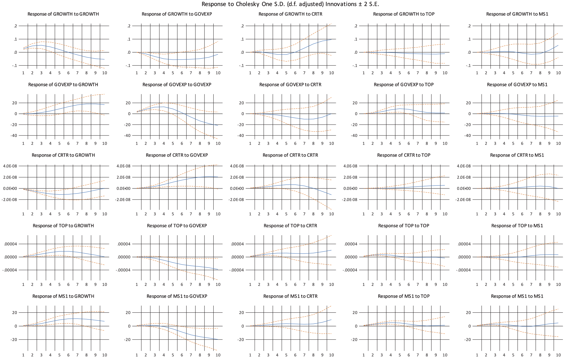
Response to Cholesky one standard innovations.

Conclusion and Policy Implications

The objective of this study was to analyze and estimate the impact of government spending volatility on economic growth in an oil-based economy covering the period 1970 to 2018. The study used HP filtering with the OLS approach. The nonlinear ARDL and the bounds Test were also applied. The aim was to gain a better understanding of the effect of government spending on real GDP growth in Saudi Arabia. Almost all existing studies ignore the effect of government spending volatility on real economic growth in oil producing countries, arguing that standard growth models do not account for measured GDP in these economies. Their results on government spending volatility negate economic growth.

This study contributes to the existing literature by applying the HP and the nonlinear ARDL approach to test the effect of government spending volatility on real GDP growth in an oil producing economy using different statistical methods. The volatility of government spending has a negative sign and is statistically significant. Equally important, a positive change in credit causes a huge increase in real growth. Moreover, a positive change in TO_t causes a decline in real GDP growth. Accordingly, the magnitude of trade openness is negative in the long run, reducing real GDP growth by 15% percent. The huge impact of TO_t in the long run can be seen in the large changes in the price of oil in the world oil market.

The ECM_t − 1 is negative and statistically significant with a value of −4.06%. The convergence from the short to the long run is 406% per year. The high adjustment process is justified by the fact that government expenditures depend mainly on oil revenues, which are affected by the large fluctuations in oil prices. The nonlinear ARDL tests, tend to support the existence of a short run and long run asymmetry between government spending and real GDP growth.

The results of the statistical tests show a consensus on the negative impact of government spending volatility on real GDP growth, which is consistent with the studies of Furceri (2007), Afonso and Jalles (2012), Iheanacho (2016), and Raju and Acharya (2020). However, there are slight differences in the impacts of the other parameters on real GDP growth. The long-run results tend to support the findings of the short-run statistical approaches. On the other hand, the IRF shows that the response of real GDP growth to government spending volatility is negative, ranging from −0.475 to −1.348 over a 10-year period. The negative association between macroeconomic volatility and real economic growth is not unique to developed countries. Therefore, less developed and oil-based countries may also be affected by such negative effects.

The study’s findings are of great importance to policymakers, researchers, and anyone interested in fiscal policy in general. For the government to implement its Vision 2030, it needs stable government revenues and thus spending. The continued instability of resources for sustained economic growth is hampering efforts to achieve higher economic goals. Policymakers should be aware that spending volatility hurts future economic prospects. Wise and rational decisions must be made to drive economic progress. Developing a local tax system and stronger stabilizing instruments will counteract the volatility of government spending. The Norwegian experience in this matter is largely commendable. The limited time series data for some of the variables that could be included, such as human capital, population growth over a long period, and segregated capital formation, forced us to neglect them. Future extensions of this model to account for symmetric and asymmetric oil price shocks are of interest. The future extensions are also applicable to the Gulf countries since they share the same economic and social environment.

Footnotes

Declaration of Conflicting Interests

The author declared no potential conflicts of interest with respect to the research, authorship, and/or publication of this article.

Funding

The author received financial support for the research, authorship, and/or publication of this article: The author would like to thank the Dean’s Office of Graduate Studies and Scientific Research at Dar Al-Uloom University in Riyadh, Saudi Arabia, for financial support.

ORCID iD

Abdulaziz H. Algaeed

References

Afonso

Furceri

(2008). Government size, composition, volatility, and economic growth (European Central Bank working paper 849). University of Lisbon.

Afonso

Jalles

J. T.

(2012). Fiscal volatility, financial crises, and growth. Applied Economics Letters, 20(1), 1821–1826. https://doi.org/10.1080/13504851.2012.667531

Aghion

Angeletos

Banerjee

Manova

(2005). Volatility and growth: Financial development and cyclical behavior of the composition of investment. Mimo, Harvard University.

Aladejare

S. A.

(2018). Resource price, macroeconomic distortions, and public outlay: Evidence from oil-exporting countries. International Economic Journal, 32(2), 199–218. https://doi.org/10.1080/10168737.2018.1481128

Albuquerque

(2011). Fiscal institution and public spending volatility in Europe. Economic Modelling, 28(6), 2544–2559.

Ali

A. M.

(2005). Fiscal policy and economic growth: The effect of fiscal volatility. Journal of Business and Economics Research, 3(5), 17–26. https://doi.org/10.19030/jber.v3i5.2772

Ali

Khan

Iqbal

(2018). Volatile discretionary public spending and economic growth: A comparative evidence of developed and developing countries. Pakistan Business Review, 20(2), 403–416.

Alley

(2016). Oil price volatility and ﬁscal policies in oil-exporting countries. OPEC Energy Review, 40(2), 192–211. https://doi.org/10.1111/opec.12074

Andrews

Rees

(2009). Macroeconomic volatility and terms of trade shocks (RBA Research Discussion Papers rdp 2009–05). Reserve Bank of Australia.

10.

Badinger

(2008). Cyclical fiscal policy, output volatility, and economic growth (CESifo Working Paper no. 2268). CESifo.

11.

Bergh

Henrekson

(2011). Government size and growth: A survey and interpretation of the evidence [IFN working paper]. Journal of Economic Surveys, 25(5), 872–897. https://doi.org/10.1111/j.1467-6419.2011.00697.x

12.

Bleaney

Halland

(2014). Natural resource exports, fiscal policy volatility and growth. Scottish Journal of Political Economy, 61(5), 502–522. https://doi.org/10.1111/sjpe.12055

13.

Çakerri

Petanaj

Muharremi

(2014). The effect of government expenditures on economic growth: The case of Albania. European Journal of Social Sciences Education and Research, 2(1), 242–254. https://doi.org/10.26417/ejser.v2i1.p242-253

14.

Churchill

S. A.

Ugur

Yew

S. L.

(2017). Does government size affect per-capita income growth? A hierarchical meta-regression analysis. Economic Record, 93(300), 142–171. https://doi.org/10.1111/1475-4932.12307

15.

Doessel

D. P.

Valadkhani

(2003). The effect of government on economic growth in Fiji. Singapore Economic Review, 48(1), 27–38. https://doi.org/10.1142/S0217590803000608

16.

Ehikioya

(2019). The impact of exchange rate volatility on the Nigerian economic growth: An empirical investigation. Journal of Economics and Management, 37(3), 45–68.

17.

Eid

Awad

(2017). Government expenditure and private sector growth in Saudi Arabia: A Markov switching model analysis. Economic Issues, 22(2), 83–104.

18.

Fernández-Villaverde

Guerrón-Quintana

Kuester

Rubio-Ramírez

(2015). Fiscal volatility shocks and economic activity. American Economic Review, 105(11), 3352–3384. http://doi.org/10.1257/aer.20121236

19.

Furceri

(2007). Is government expenditure volatility harmful for growth? A cross-country analysis. Fiscal Studies, 28(1), 103–120. https://doi.org/10.1111/j.1475-5890.2007.00049.x

20.

Furceri

Ribeiro

(2008). Government spending volatility and the size of nations (European Central Bank Working Paper Series no. 924). European Central Bank.

21.

Garayva

Tahirova

(2016). Government spending effctiveness and the quality of ﬁscal institutions (MPRA Paper no. 72177). MRPA. https://mpra.ub.uni-muenchen.de/72177

22.

Gelb

(1981). Capital-importing oil exporters: Adjustment issues and policy choices (World bank staff Working Paper no. 475). 1–51. World Bank.

23.

Güreşçi

(2018). Effects of macroeconomic volatility on economic growth: Evidence from European Union countries. International Journal of Management Economics and Business, 14(3), 591–599. https://doi.org/10.17130/ijmeb.2018343112

24.

Hodrick

Prescott

(1997). Post war U. S. business cycles: An empirical investigation. Journal of Money, Credit and Banking, 29, 1–16.

25.

Iheanacho

(2016). The contribution of government expenditure on economic growth of Nigeria disaggregated approach. International Journal of Economics and Management Sciences, 5(5), 1–8. https://doi.org/10.4172/2162-6359.1000369

26.

Kim

C. -J.

Nelson

C. R.

(1999). Has the US economy become more stable? A Bayesian approach based on a Markov-Switching model of the business cycle. Review of Economics and Statistics, 81(4), 608–616. https://doi.org/10.1162/003465399558472

27.

Koh

W. C.

(2017). Fiscal policy in oil-exporting countries: The roles of oil funds and institutional quality. Review of Development Economics, 21(3), 567–590. https://doi.org/10.1111/rode.12293

28.

Leibrecht

Scharler

(2012). Government size and business cycle volatility; how important are credit constraints? (University of Lüneburg Working Paper Series in Economics 237). University of Lüneburg. http://www.leuphana.de/institute/ivwl/publikationen/working-papers.html

29.

Maluleke

(2017). The determinants of government expenditure: Analysis of the empirical literature from 1995 to 201. Acta Universitatis Danubius, 13(2), 212–219.

30.

Manganelli

Popov

(2015). Financial development, sectoral reallocation, and volatility: International evidence. Journal of International Economics, 96(2), 323–337. https://doi.org/10.1016/j.jinteco.2015.03.008

31.

Mohammad

Wasti

Lal

Hussain

(2009). An empirical investigation between money supply, government expenditure, output and prices: The Pakistan evidence. European Journal of Economics, Finance and Administrative Sciences, 17, 60–68.

32.

Neicheva

(2006). Non-Keynesian effects of government expenditure on output in Bulgaria: An HP filter approach. Post-Communist Economies, 18(1), 1–12. https://doi.org/10.1080/14631370500505081

33.

Nworji

Okwu

Obiwuru

Nworji

(2012). Effects of public expenditure on economic growth: A disaggregated time series analysis. International Journal of Management Sciences and Business Research, 1(7), 1–15.

34.

Nyasha

Odhiambo

N. M.

(2019). Government size and economic growth: A review of international literature. SAGE Open, 9(3), 1–12. https://doi.org/10.1177/2158244019877200

35.

Olubokun

Ayooluwade

Olumide

(2016). Government expenditure, inflation rate and economic growth in Nigeria (1981–2013): A vector autoregressive approach. Romanian Journal of Fiscal Policy, 7(1), 1–12.

36.

Onyimadu

(2017). Macroeconomic volatility and economic growth: Evidence from selected African countries (MPRA Paper no. 7700). MPRA. https://mpra.ub.uni-muenchen.de/77200/

37.

Pham

T. A.

(2018). Policy volatility and growth. Portuguese Economic Journal, 17(2), 87–97. https://doi.org/10.1007/s10258-018-0144-6

38.

Raju

Y. N.

Acharya

(2020). Revisiting the volatility-growth relationship: Some cross-country evidence 1978–2017. Cogent Economics and Finance, 8(1), 1826655. https://doi.org/10.1080/23322039.2020.1826655

39.

Ramey

(1995). Cross-country evidence on the link between volatility and growth. American Economic Review, 85(5), 1138–1151.

40.

Rodrigues da Silva

Tabak

Cajuerio

Fazio

(2018). Economic growth, volatility, and their interaction: What is the role of finance (Banco central do Brazil working Papers no. 474). Banco central do Brazil.

41.

Sadeghi

(2017). Oil price shocks and economic growth in oil-exporting countries: Does the size of government matter? (IMF working paper no 17(287)). IMF. https://doi.org/10.5089/9781484335390.001

42.

Sahu

Nirola

(2019). The interactive impact of government size and quality of growth-evidence from the states of India. Heliyon, 5, e01352. https://doi.org/10.1016/j.heliyon.2019.e01352

43.

Shin

Greenwood-Nimmo

(2014). Modelling asymmetric cointegration and dynamic multiplier in a nonlinear ARDL framework. In Sickles

R. C.

Horrace

W. C.

(Eds.), Festschrift in honor of Peter Schmidt: Econometric methods and applications (pp. 281–314). Springer.

44.

Stounaras

(2010). Fiscal expenditure and trading implications for economic growth: The case of Greece. IUP Journal of Public Finance, VIII(3), 49–72.

45.

Surjaningsih

Utari

G. A. D.

Trisnanto

(2012). The impact of fiscal policy on the output and inflation. Bulletin of Monetary Economics and Banking, 14(4), 367–396. https://doi.org/10.21098/bemp.v14i4.409

46.

Turan

Iyidogan

(2017). Growth volatility and government expenditure in low- and middle-income countries: A dynamic panel analysis. Transylvanian Review of Administrative Sciences, 51, 123–138. https://doi.org/10.24193/tras.51E.8

47.

van Ingen

Wait

Kleynhans

. (2014). Fiscal policy and revenue management in resource-rich African countries: A comparative study of Norway and Nigeria. South African Journal of International Affairs, 21(3), 367–390. http://doi.org/10.1080/10220461.2014.968200

48.

Wickremasinghe

G. B.

(2005). Efficiency of foreign exchange markets: A developing country perspective. SSRN Electronic Journal, 10(1), 1–17. https://doi.org/10.2139/ssrn.609285

Government Spending Volatility and Real Economic Growth: Evidence From a Major Oil Producing Country,Saudi Arabia,1970 to 2018

Abstract

Keywords

Introduction

Review of Theoretical and Empirical Literature

Material and Methodology

Description of Data

The Model

Estimation and Discussion

The Unit Root Tests

The OLS Regression Models Results

The Nonlinear ARDL Model

The Nonlinear ARDL Regression Model and Diagnostic Tests

Diagnostic Tests

The Impulse Response Function

Conclusion and Policy Implications

Footnotes

Declaration of Conflicting Interests

Funding

ORCID iD

References