
Abstract
This study aims to investigate the determinants of financial development and explore the impact of population and GDP on financial development. Annual time series data covering the period from 2000 to 2022 were used, focusing on variables including the number of listed companies (NLC) and bank Z-score (BZS) as financial development indicators, and urban population (UP), rural population (RP), and Gross Domestic Product as determinants. Unit root tests and the Auto Regressive Distributed Lag (ARDL) bound technique are used to find the long-run co-integration relationship of the model. The Vector Error Correction (VEC) technique detects short-run relationships. The stability and reliability of the models are assessed through diagnostic tests, recursive analysis, and dynamic ordinary least squares. Granger causality analysis is employed to examine the causal relationships between the variables. The results indicate that population and GDP significantly affect the NLC and BZS in the long term, and a negative short-term relationship is observed between the financial indicators and explanatory variables. CUSUM and CUSUMSQ plots confirm the effectiveness of the modeling, and DOLS supports the reliability of the ARDL models. Granger causality suggests unidirectional causality from population to NLC and BZS, while NLC and BZS are found to be Granger causes of GDP. Based on the impact of population on financial development, policymakers are recommended to focus on strategies for population growth, including healthcare improvements, education access, and family planning programs. Additionally, diversifying economies, promoting sustainable growth, and implementing favorable economic policies are suggested to enhance financial development.
Plain language summary
This research investigates what influences financial development and how factors like population size and Gross Domestic Product (GDP) impact financial growth. Data from 2000 to 2022 was analyzed, focusing on the number of listed companies and bank health as indicators of financial development, along with urban and rural population numbers and GDP as determining factors. Various statistical techniques were used to analyze the data, looking at both long-term relationships and short-term dynamics. The results show that population size and GDP have a significant impact on financial development over the long term, with some negative effects in the short term. The study used different tests to ensure the models were stable and reliable. The findings suggest that population size plays a crucial role in financial development. To improve financial growth, policymakers are advised to concentrate on strategies that support population growth through measures like healthcare enhancements, better education access, and family planning programs. It is also recommended to diversify economies, promote sustainable growth, and implement favorable economic policies to enhance financial development further.
Introduction
Despite the exceptional circumstances due to COVID-19, which greatly affected the global economy and cast a shadow on the Saudi economy during 2020, the Saudi banking sector still enjoys strength and stability (Orlando & Bace, 2021). This comes as a reflection of the procedures and measures that the Saudi Central Bank and Saudi banks worked together, which had a major role in mitigating the negative effects (Al-Humoud, 2020). Saudi Arabia, a member country of the Financial Stability Board and G20, has successfully implemented Basel III and is currently in the process of implementing resolution legislation (Orlando & Bace, 2021). The potential of COVID-19 on the private sector and the banking sector, as indicated by financial toxicity indicators, as the capital adequacy rate rose to 20.3%, which is higher than the international requirements represented by the requirements of the Basel Committee, and the assets of banks increased by 13.2%, and their deposits grew by 8.2%. Commercial banks showed good performance in 2020, with total assets increasing 13.2%, compared to a growth of 9.7% in 2019 (SCB, 2024).
With over 34 million people in 2024 (GASTAT, 2024), Saudi Arabia is a leading nation in the Middle East. Alongside its thriving population, the country boasts significant financial development. The urban population in Saudi Arabia was estimated to be over 32 million people in 2023, reflecting a 1.54% increase compared to 2021 (GASTAT, 2024). On the other hand, the rural population in Saudi Arabia is estimated to be nearly 6 million people in 2022, showing a decline of 0.17% from 2021 (FAO, 2024). According to an estimation of GASTAT (2023), the real GDP for the year 2023 decreased by 0.9% compared to the year 2022. This decrease resulted from the decline in oil activities by 9.2% despite the growth of non-oil and government activities by 4.6% and 2.1%, respectively
Saudi Banking System
According to Elbadry (2018), Saudi Arabia boasts the largest economy in the Middle East and North Africa region. Consequently, the banking sector in Saudi Arabia stands out as a significant and promising industry when compared to its counterparts in the area. In Saudi Arabia, the financial system comprises various entities, including banks, financial companies, quasi-government funds, and public credit suppliers (S. Z. Ahmed, 2021; Banafe & Macleod, 2017). The regulatory oversight for both Sharia-compliant banks, which adhere to Islamic principles, and conventional banks, which follow traditional banking practices, falls under the responsibility of the Saudi Arabian Monetary Authority (SAMA). SAMA operates within a unified regulatory framework to ensure effective regulation and supervision of the banking sector (Alrabiah & Drew, 2022). Economic growth in developed economies positively influences banking performance and strengthens financial systems (Obiora et al., 2022; Rousseau & Sylla, 2003). The banks in the region maintain conservative leverage levels, strong capitalization, high liquidity, sufficient provisioning, and profitable operations. However, their reliance on government spending exposes them to potential challenges, particularly during periods of low oil prices. Additionally, there are concerns regarding liquidity due to these economic conditions, and banks face concentration risk in their lending activities. To mitigate these potential risks and maintain the financial system’s stability, authorities are considering implementing macroprudential regulations (Kahou & Lehar, 2017). These rules limit system-wide risks and promote a more resilient banking sector. By imposing prudential measures and regulations, the goal is to enhance the overall resilience of the financial system and safeguard against potential vulnerabilities (Banafe & Macleod, 2017). From Figure 1, the numbers of the listed companies showed a slightly increasing rate, while the GDP and bank Z-score fluctuated during the period 2000 to 2022.
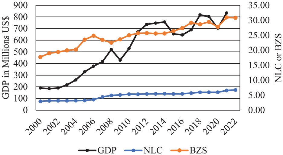
Financial Development and GDP Trends in Saudi Arabia (2000–2022).
Regarding the population size, as observed in Figure 2, during the last decades, the rural population has decreased while the urban population has increased in Saudi Arabia. This can be attributed to the fact that urban areas in Saudi Arabia offer a greater range and abundance of job opportunities compared to rural areas. The growth of industries, commerce, and services supported by financial development has created a favorable environment for urbanization. As the financial sector expands and diversifies, it contributes to the overall development of urban areas and acts as an incentive for the migration of people from rural to urban regions in search of better employment prospects and higher wages.
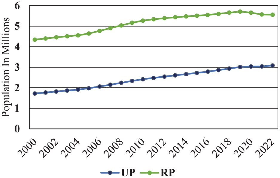
Population trend in Saudi Arabia (2000–2022).
Saudi Arabia depends heavily on oil incomes in its economy; nevertheless, the fluctuations in global oil prices and demand can significantly affect the Saudi economy. Saudi Arabia has implemented strategies to diversify its economy and promote the growth of non-oil sectors. For instance, boosting tourism services, increasing manufacturing, and enhancing financial services, technology, and agriculture required significant investments and employment. Therefore, strategies and policies have been taken to enhance revenues and reduce expenditures, such as imposing a value-added tax and dropping government subsidies from some sectors. However, there is still a need to improve the management of financial resources and develop sustainable sources of revenue, and this is achieved through the Kingdom’s Vision 2030 (The Saudi Vision, 2023), which aims to achieve sustainable development, economic diversification, attract investments, and develop human skills. As Saudi Arabia transitions under Vision 2030, financial sector reforms are aimed at enhancing inclusion, market efficiency, and resilience. However, several challenges hinder its sustainable development. These challenges can be categorized into: A. Internal challenges: The economy’s heavy reliance on oil revenues makes financial development vulnerable to oil price shocks. Non-oil sectors remain underdeveloped, limiting alternative financial growth sources. B. External challenges: Global economic shocks, such as recessions and trade disruptions, also impact Saudi financial markets. Although the country has opened its markets, foreign investment remains constrained due to bureaucratic hurdles. This study offers valuable insights into the relationship between GDP, population growth, and financial development sustainability in Saudi Arabia. Understanding how GDP volatility affects financial markets can assist in suggesting risk management strategies. Rapid urbanization in Saudi cities increases demand for housing finance, capital markets, and investment products. Furthermore, this study can contribute to economic policy, financial research, and practical applications that support a stable, inclusive, and resilient financial system in the Kingdom. Studying GDP and population growth helps forecast financial resilience and potential risks in regional and global financial markets. Besides investigating the GDP and population as determinants of financial development in Saudi Arabia is not just a domestic concern; it offers global insights into emerging market dynamics, financial stability, foreign investment, financial inclusion, and sustainability. This research can help policymakers, investors, and financial institutions worldwide develop more resilient and inclusive financial systems.
Most studies on financial development in Saudi Arabia focus on monetary policies, oil dependence, and stock markets (Abdou et al., 2024; Ben Amar, 2022). Also, limited research explores the combined effect of GDP and population growth on financial sustainability (Alabdulwahab, 2021; Samargandi et al., 2014). This study fills this gap by providing empirical evidence on how macroeconomic and demographic factors interact with financial sector growth. Likewise, the findings can serve as a case study for other Gulf Cooperation Council (GCC) countries and oil-dependent economies. Therefore, this study aims to investigate the determinants of financial development and how the degree of the impact of GDP and population has been impacted.
The rest of the study is structured as follows: Section 2 presents the literature review; Section 3 describes the data and econometric methods; Section 4 presents the estimations, findings, and discussions, and Section 5 concludes the study with policy implications, recommendations, and limitations.
Theoretical Framework & Literature Review
Financial Development
The theoretical framework of financial development explores how financial systems encompassing institutions, markets, and instruments evolve to efficiently allocate resources, manage risks, and drive economic growth (Fry, 1995, 1998). Early theories, notably those of McKinnon (1973) and Shaw (1973), argued that financial liberalization fosters higher savings and investment, ultimately accelerating economic growth. A substantial body of theoretical and empirical research demonstrates that financial development significantly influences economic performance (Ductor & Grechyna, 2015). Adu et al. (2013) suggest that the overall impact of financial development on growth is susceptible to the choice of indicators.
Understanding the determinants of financial development is crucial, as research indicates that financial development is not merely a byproduct of economic progress. Financial development is influenced by a complex interplay of institutional, economic, structural, and external factors (M. A. Khan et al., 2022; Marques & Morgan, 2021). Countries that implement sound policies, strengthen institutions, and embrace financial innovation tend to experience more robust financial development, leading to greater economic growth and stability.
Economic Growth and Financial Development Sustainability
Economic growth plays a crucial role in sustaining financial development through multiple interrelated mechanisms (Alhassan et al., 2022; Maharajabdinul, 2024). As economies expand, household incomes typically increase, leading to higher savings rates and a larger pool of funds for financial intermediation, thereby boosting credit and investment activities. Additionally, sustained growth often drives structural transformation, particularly the expansion of non-agricultural sectors, which raises the demand for more advanced and diverse financial services (De Gregorio & Guidotti, 1995). This procedure promotes the expansion and flexibility of financial markets (Arestis & Demetriades, 1997). Moreover, economic growth enhances government fiscal capacity, enabling greater investment in regulatory institutions, legal frameworks, and financial infrastructure, opening elements for long-term financial development.
Significantly, there exists a positive feedback loop, where financial development further stimulates economic growth by improving capital allocation, promoting innovation, and supporting entrepreneurship, thereby reinforcing the financial system’s sustainability (Bernier & Plouffe, 2019). Furthermore, sustained economic growth empowers governments and central banks to invest in financial infrastructure, contributing to long-term financial system stability and depth. Based on this dynamic analysis, the following hypothesis is proposed:
There are several probable reasons why the impact of GDP on financial development is stronger in the long run than in the short run. Economic growth may not immediately lead to substantial financial sector advancement in the short term due to institutional, regulatory, and infrastructural constraints. However, over time, sustained GDP growth enables greater investment in financial infrastructure, encourages policy and regulatory reforms, and promotes improvements in financial knowledge and market development. Moreover, as economies increase, structural transformations enhance the demand for financial services, while confidence in financial institutions gradually strengthens. These long-term, cumulative effects clarify why the connection between GDP and financial development tends to be more significant over a long period.
Population Growth and Financial Development Sustainability
Population growth influences the sustainability of financial development through demand and supply-side dynamics. Population growth influences financial development and sustainability by expanding the client base for formal and digital financial institutions. As the population grows, particularly in urban areas, there is a growing demand for financial services such as banking, insurance, allowances, and digital payment systems, prompting financial institutions to expand and innovate. In many developing countries, this growth results in a youthful demographic, which tends to be more receptive to financial technologies, driving the adoption of inclusive, tech-driven financial services (Esposito et al., 2025; Mori, 2023). However, rapid population growth can also present challenges; if not matched by adequate economic growth, it may lead to underemployment, poverty, and financial exclusion (Zhang, 2016). To ensure sustainable financial development, it is essential to establish scalable financial infrastructure, supportive regulatory frameworks, and targeted financial literacy initiatives that promote broad-based access and long-term system stability. Based on this dynamic analysis, the following hypothesis is proposed:
There are several possible reasons why population growth positively influences financial development in Saudi Arabia. It can lead to increased domestic savings, greater demand for diverse financial products, modernization of public financial services, and expansion of the labor market. Together, these factors contribute to a more dynamic and inclusive financial environment that supports the sustainable long-term growth of the financial sector.
Literature Review
Several studies have utilized the Autoregressive Distributed Lag (ARDL) econometric approach to examine the factors influencing financial development across diverse economies. For instance, Asratie (2021) examined the determinants of financial development in Ethiopia by applying the ARDL estimation technique. Find that the broad money supply model is positively influenced by factors such as the political freedom index, economic growth, and trade openness, both in the short and long run. Conversely, it is negatively affected by interest rates and reserve requirements. In the same context, Najimu (2019) utilized the ARDL approach to analyze the factors contributing to financial development in Ghana. The examined results confirmed a unique cointegrating relationship between financial development, trade openness, inflation, per capita income, reserve requirement, and government borrowing. Further, their study investigated that inflation, interest rate, and reserve requirement exerted negative and statistically significant effects on financial development in the short and long run. Z. Ahmed et al. (2021) study symmetric and asymmetric ARDL methods to examine the nexus between ecological footprint, economic globalization, economic growth, and financial development, controlling for Japan’s population density and energy consumption. The findings reveal the long-run asymmetric and symmetric relationship of variables with the ecological footprint.
Other studies used different econometric methods to investigate the determinants of financial development, focusing on social, economic, and environmental factors. Liu et al. (2021) examined the factors that contributed to the development of digital financial inclusion in urban and rural areas. They utilized the fixed-effect model and panel threshold technique to analyze the available data. The empirical findings highlighted the existence of a threshold effect in the relationship between financial development and digital financial inclusion. A study applied the dynamic panel System Generalized Method of Moments (System GMM) approach, which exposed that income level positively influences financial development, and the exchange rate encourages financial depth and lending activities. Furthermore, the study results indicated that inflation stimulates bank private credit and reduces the depth of the financial sector (Abubakar & Kassim, 2018). Another study performed in Pakistan aimed to investigate the determinants of financial development using regression analysis and correlation methods. The empirical findings indicate that inflation, trade openness, market capitalization, investment rate, and interest rate have a significant impact on financial development (Yang & Shafiq, 2020). Aluko and Ibrahim (2020) investigated the macroeconomic determinants of financial institutions’ development in sub-Saharan Africa. Using the two-step system generalized method of moments(GMM) dynamic panel model estimation approach, the results reveal that trade openness, income, and government expenditure are positive determinants of financial institutions’ development, while higher inflation inhibits improvement in financial institutions. On the other hand, H. U. R. Khan et al. (2019) examined the effect of financial development indicators on natural resource markets and applied the GMM estimator. The results show that the distortion in commodity prices impacted energy and natural resource markets.
Fakher et al. (2022) used a composite environmental quality index, a composite financial development index, and a composite trade share measure to represent environmental quality, financial development, and trade openness, respectively. The study used a joint of econometric methods, Continuously Updated Fully Modified (CUFM), Continuously Updated Bias Corrected (CUBC), and Dumitrescu Hurlin (DH) causality to examine the nature of the linkage between the study’s variables. The result indicated that financial development upsurges economic growth in high and low-income nations.
A study used panel data to investigate the relationship between financial development and economic growth using Panel Ordinary Least Squares (OLS) and Panel Fully Modified Least Squares (FMOLS) methods in developing countries. The results of the study provide evidence of a direct relationship between financial development and growth in developing countries (Ekanayake & Thaver, 2021). Besides, Ibrahim and Sare (2018) observed the determinants of financial sector development and investigated whether trade openness and human capital interaction can explain financial development. Findings show that, while human capital robustly influences financial development, trade openness robustly matters more for private credit than domestic credit.
In the context of GCC countries, several studies were conducted during the last decades. A study in Saudi Arabia applied the bootstrap approach to the ARDL model and proved that financial development and ICT diffusion positively affected economic development (Gheraia et al., 2022). In another study performed in Saudi Arabia, a Computable General Equilibrium (CGE) model was employed to investigate the impact of the COVID-19 pandemic on the Saudi Arabian economy and financial situation. The study revealed that government social grants played a crucial role in alleviating the hardships faced by the most vulnerable segments of the population amidst the pandemic (Alharbi, 2024).
A study conducted in the Gulf Cooperation Council (GCC) countries seeks to advance current understanding by examining how institutions influence the correlation between financial progress and carbon emissions, utilizing a dynamic GMM model. Financial system advancement was assessed based on the expansion of the banking sector and the development of financial markets. The results indicate that corruption control, high-quality regulations, and a robust rule of law play a pivotal role in mitigating the environmental impact on the financial development (Ghardallou & Abaalkhail, 2024).
Among the literature mentioned above, almost all studies have tried to examine the relationship between financial development using money supply, inflation rate, interest rate, reserve requirement, oil price, and bank private credit as financial development factors, and connected them with economic growth and trade openness. However, a few studies investigated the relationship between the bank Z-score, the number of listed companies, and the rural and urban population (Ghassan & Guendouz, 2019; Li et al., 2020; Loc et al., 2024). In comparing our study with the earlier studies in other GCC countries using the ARDL model, which have only considered limited variables, this study’s inclusion of urban and rural population factors with financial stability indicators provides a broader view. Additionally, by combining ARDL and ECM models, the study captures both short- and long-term financial dynamics, which many prior studies addressing only one timeframe fail to do. The paper’s focus on specific economic contexts, like the differentiated impacts of urban and rural populations on financial stability in Saudi Arabia, and its attention to oil dependency effects, distinguishes it further.
Therefore, this study tries to fill a gap in the literature review in this context. Besides, our study holds a significant effect as it focuses on the determinants of a bank’s Z-score and the number of listed companies, examining GDP and population as key factors. By exploring this relationship, we gain deeper insights into the intricate interplay between the banking sector, economic indicators, and market dynamics. This study allows us to evaluate the performance and stability of banks more comprehensively. Furthermore, our study offers valuable assistance to investors, policymakers, and analysts in assessing investment opportunities. By considering the impact of GDP and population on the bank Z-score and the number of listed companies, stakeholders can make more informed decisions. They can track economic development, identify promising investment prospects, and formulate well-informed policies that respond to the dynamics of capital markets.
Materials and Methods
This section briefly describes the data types and models adopted for the study.
Data and Descriptive Statistics
To support Saudi Arabia’s Vision 2030, Saudi Arabia was selected as a case study for this research for achieving a program of financial sector development. The current study is based on the annual time series data covering the period (2000–2022) collected from the WB (2024a, 2024b). The selected variables involve the number of listed companies (NLC) per 1,000,000 people and bank Z-score (BZS) in (%) act as the Key of the financial sector, financial development indicators “dependent variables,” urban population (UP) in (person), rural population (RP) in (person) and Gross domestic product (GDP) in (US$) represent the financial development determinants “independent variables.” The reason for choosing the number of listed companies (NLC) and bank Z-score (BZS) as financial development indicators in our study is based on their reflection on the strength of the stock market, indicating the level of financial market development. On the other hand, the bank Z-score measures the financial health and stability of the banks, providing insights into the overall strength of the banking sector (Arzova & Sahin, 2024). The choice of NLC and BZS as dependent variables in our research may have implications for policymakers and regulators (Laeven & Levine, 2009). Likewise, the rationale for selecting the independent variables is grounded in their established relationship with financial development; for example, urbanization is strongly associated with the expansion and accessibility of financial services. Urban areas tend to have a higher concentration of economic activities, financial institutions, and infrastructure, which can boost financial development. By incorporating urban population (UP) as a determinant, we can explore how the degree of urbanization influences financial development in the context of our study in Saudi Arabia. Furthermore, rural populations may have different financial requirements and access to financial services compared to urban populations. Similarly, by including GDP as a determinant, we can examine how the level of economic development connects to financial development in Saudi Arabia.
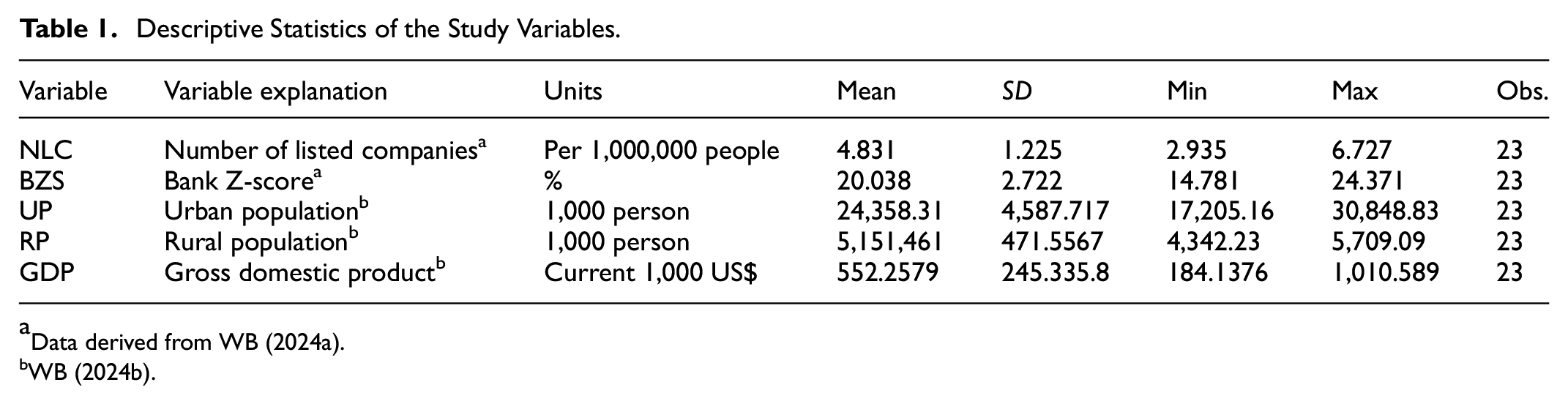
Abbreviations, variable explanations, and descriptive statistics for key variables used are presented in Table 1. A high SD of population data could be caused by factors such as variations in age, income, education, occupation, or any other property being measured. Similarly, a high SD of GDP data could be caused by several factors, including changes in government policies, shifts in global economic conditions, fluctuations in key industries, or other internal or external factors affecting the economy.
Descriptive Statistics of the Study Variables.
Data derived from WB (2024a).
The dataset was transformed into a natural logarithm form to challenge the problems of autocorrelation and heteroscedasticity and deliver estimated results with small coefficient values, which can be beneficial for analysis and interpretation.
Unit Root Tests
Before starting data analysis, preliminary assessments were performed to ensure the validity and reliability of the analytical techniques employed. The important concept in this regard is unit root tests. Dickey and Fuller (1979, 1981) and Phillips and Perron (1988) tests were applied to determine whether a time series variable is stationary (i.e., mean-reverting) or non-stationary (i.e., affected by unit roots). The null hypothesis (H0) for these tests suggests that the series is non-stationary, contrasting it with the alternative hypothesis (H1) that the series is stationary.
ARDL Cointegration Bounds Testing Approach
The ARDL estimation technique was developed by Pesaran and Shin (1995) to analyze the short-run and long-run associations between the study variables. The model offers unbiased and efficient estimations (Malik et al., 2020; Menegaki, 2019). The uniqueness of this model lies in its flexibility regarding variable integration orders; it could be integrated at the level I(0) and the first difference I(1); however, the existence of I(2) would make the ARDL inappropriate.
Several investigators used this technique to examine the connection between financial development, economic growth, energy, trade, and the environment (Z. Ahmed et al., 2021; Assi et al., 2021; M. I. Khan et al., 2020; Qamruzzaman & Wei, 2018; Usman et al., 2023). However, our study examines the connection between financial development, rural, urban, and GDP (economic growth) using ARDL.
According to Sam et al. (2019), the single ECM (error correction model) equation is written for NLC and BZS as:
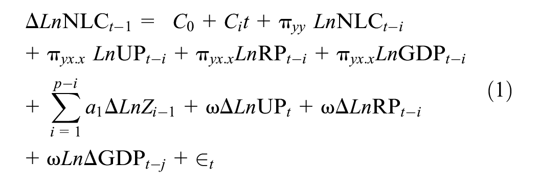

Where;
Furthermore, the different cointegration and non-cointegration cases involving NLC and BZS are tested within the ARDL equation. So the ARDL model was estimated for NLC and BZS and
and takes the following equation
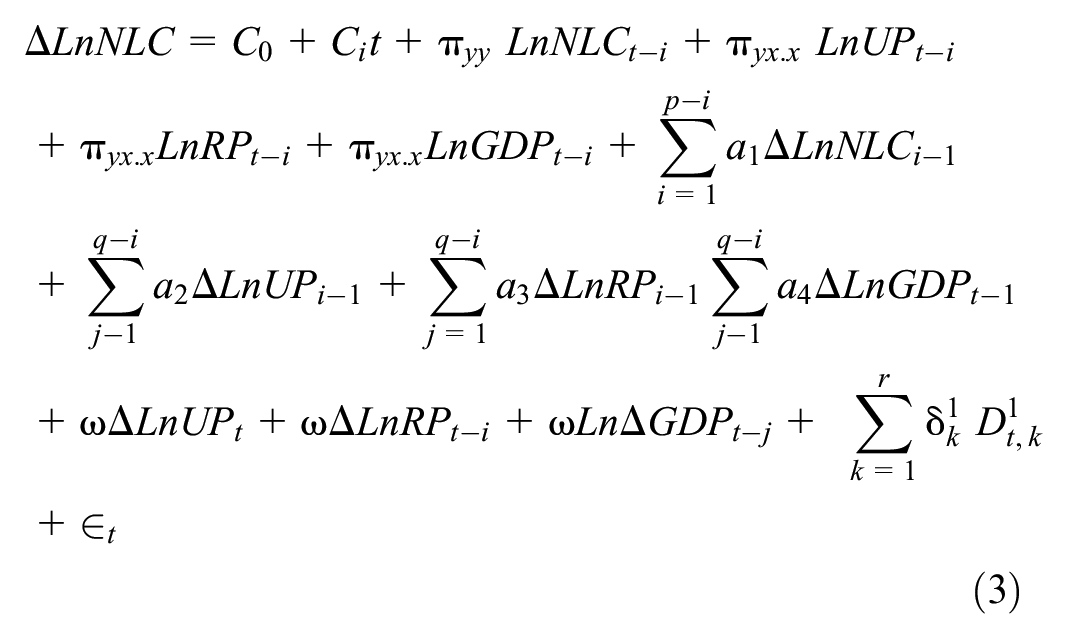

The k is the dimension of the forcing variables, and r is the forcing variable cointegration rank. Where
Where;
The bound test was used to detect the cointegration of the variables. The appropriate values for the maximum lags of n will be determined by applying the Akaike Information Criterion (AIC).
Model Stability and Diagnostic Tests
Ensuring the dynamic stability of any model with an autoregressive structure is required (Senyuk et al., 2023). The stability of the model is checked by applying the recursive method proposed by Peseran and Peseran (1997). Diagnostic tests were conducted to check model reliability. In that context, the Breusch-Godfrey test was used to check autocorrelation; the Breusch-Pagan test was used for testing heteroskedasticity, and for the normality test, we used Jarque-Bera (JB) to test whether the data is symmetrically distributed normally around its mean or not.
Granger Causality Test
We used the Granger causality (Granger, 1969) approach to detect the existence of causality between the selected variables. This test is justified as it helps determine the direction and strength of influence among these variables.


Whereas: PG could be urban population (Ln UP), rural population (LnRP), or LnGDP; respectively,
The ARDL model, however, is a powerful tool for analyzing relationships between variables in a time series context, involving several limitations. Some key limitations of the ARDL model require specifying the appropriate lag lengths, and selecting incorrect lag orders might lead to biased parameter estimates and inaccurate inference. Also, in the presence of endogeneity, the estimated coefficients may be biased and inconsistent (Kripfganz & Schneider, 2023). Also, the ARD has a limited dynamic specification (captures short-term and long-term dynamics) but may not allow for more complex dynamic relationships that extend over longer periods. Finally, difficulty in handling structural breaks, the ARDL model can be sensitive to structural breaks in the data, and detecting and appropriately addressing these breaks can be challenging (Ghouse et al., 2018; Murshed et al., 2021)
Finally, estimating the ARDL model with multiple lags and variables can increase model complexity and computational challenges, especially when dealing with large datasets. Therefore, addressing these limitations through robustness checks can help mitigate potential issues and improve the reliability and validity of the findings derived from the ARDL framework.
For robustness, the ARDL’s results of the dynamic ordinary least squares (DOLS) models were used to estimate the long-run connections between the selected variables. We chose this method as it provides consistent and efficient estimates of the long-run coefficients. Ultimately, to assess model accuracy and predictive power, we plot the residuals of the selected variables to identify any patterns or differences between the predicted values and the observed values.
Results and Discussions
Unit Root Testing
The Augmented Dickey-Fuller (ADF) and the Phillips–Perron unit root testing results are displayed in the following Table 2. Figures 1 and 2 demonstrate the presence of emerging trends in certain series, suggesting the necessity of incorporating a linear trend in the unit root tests. Given that the ARDL bounds test permits time series to be categorized as I(0) or I(1) only, a series of unit root tests was carried out to confirm that the variables under examination do not exhibit an integration order greater than one.
Unit Roots Test Results.

Source. Authors’ calculations (2024).
Note.p-Value for Z(t) in the bracket ().
At 1% = −4.380, at 5% = −3.600, and 10% = −3.240.
At 1% = −3.750, at 5% = −3.000 and at 10% = −2.630.
The stationarity test results, based on the Dickey-Fuller (DF) and Phillips–Perron (PP) methods with trend and intercept specifications, indicate that most variables in the analysis are non-stationary. Specifically, NLC, BZS, and GDP fail to reject the null hypothesis of a unit root across all specifications, with test statistics falling short of the critical values at the 1%, 5%, and 10% significance levels. This confirms that these series are non-stationary in the level form, but they are stationary at the first difference. On the other hand, UP and RP demonstrate stationarity only under the intercept specification of the Dickey-Fuller test, where their test statistics exceed the 5% and 10% critical thresholds. Given a data mix of I(0) and I(1), we approved applying the ARDL approach.
ARDL Estimation Results
The Akaike Information Criterion (AIC) was used to determine the optimum lag length of the model. The selected ARDL models have different lag length configurations for the dependent variables NLC and BZS. Considering the NLC model, the optimal lag lengths are 1, 2, 2, and 2 for NLC, UP, RP, and GDP, respectively. On the other hand, the BZS model has an optimal lag length of 3 for all variables: BZS, UP, RP, and GDP.
Diagnostic Tests of the ARDL Model
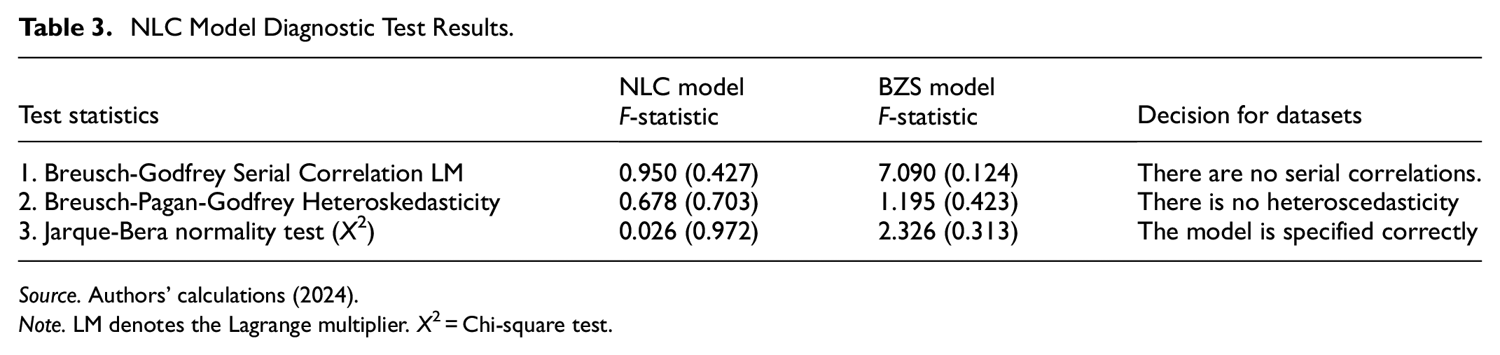
As illustrated in Table 3, the ARDL NLC and BZS models’ performance is satisfactory, as they meet all the diagnostic criteria and requirements. The estimated F-statistics regarding serial correlation (Breusch-Godfrey Serial Correlation LM tests) and heteroscedasticity (Breusch-Pagan-Godfrey test) reject the null hypothesis as F (p-values) are greater than 5%. Likewise, the normality (Jarque-Bera test) also rejects the null hypothesis that the regressors have zero coefficients (X2 = 0.026 with p = .972 for the NLC model and X2 = 2.326 with p = .313 for BZS). These results indicate that the ARDL for NLC and BZS models’ assumptions related to these aspects are met, enhancing the NLC and BZS models’ validity and reliability. Most of the studies using ARDL to investigate the determinants of the financial development indicators showed the absence of serial correlation, heteroscedasticity, and normal distribution of their data sets (Z. Ahmed et al., 2021; Mehta et al., 2021; Saleem et al., 2021).
NLC Model Diagnostic Test Results.
Source. Authors’ calculations (2024).
Note. LM denotes the Lagrange multiplier. X2 = Chi-square test.
ARDL Cointegration Bounds Testing Results
Since the values of the computed F-statistic exceed the upper bound of the critical F-statistic (5.816) for the NLC and 5.966 for the BZS models at the significance level of critical values 1%, however, the computed T-statistic exceeds the upper bound of a critical T-statistic (−3.44) for the NLC and −3.613 for the BZS models at the significance level of critical values 5%, and 10%. We can conclude that there is evidence of a long-run relationship between the time series of the NLC and the BZS model (Table 4).
Bounds Testing Values of the NLC and BZS Model.

Source. Authors’ calculations (2024).
The results in Table 5 show that the coefficients for LnUP, LnRP, and LnGDP significantly affect the LnNLC. The main findings indicate that LnRP and LnGPD have statistically significant positive effects on NLC, which means that a 1% increase in LnRP and LnGPD would cause LnNLC to rise 282.396% and 0.338%, respectively. However, LnUP could decrease by 283.435% when the LnUP increases by 1% in Saudi Arabia.
Long-run ARDL and Bounds Testing Critical Values of the ARDL Model.

Source. Authors’ calculations (2024).
Note. Prob (F-statistic).
, **, and * at 1%, 5%, and 10%, respectively.
In the context of the LnBZS model, the analysis reveals that the current value of LnUP has a marginally significant positive relationship with the LnBZS at the 5% level, indicating that an increase in LnUP is associated with a higher value of the LnBZS variable (p = .06 at the 10% level of significance). Given the interpretation in the economic and financial context of these results, it may suggest that banks in urban areas tend to be more stable due to larger customer bases, more diversified financial activities, and greater access to financial services and credit markets. Comparing our results with Kayani et al. (2020) confirmed significant long-term positive relationships between financial development and urban population with CO2 emissions.
Furthermore, the lagged values of LnUP (−1) and LnUP (−2) show a marginally significant negative relationship with the LnBZS, suggesting that past decreases in LnUP may have a modest impact on reducing the value of the LnBZS. However, the lagged value of LnUP (−3) stands out as highly significant, indicating a strong positive relationship with the BZS. This finding implies that an increase in LnUP three periods ago substantially influences the current value of the LnBZS, potentially leading to a notable increase in its value.
The current value of LnGDP and the lagged values (−1) and (−3) of LnGDP have an insignificant impact on the LnBZS. Its coefficient is not statistically significant. However, the lagged value of LnGDP (−2) shows a marginally significant positive relationship with the LnBZS (p = .07 at a 10% significance level). Our results agreed with Çetenak et al. (2023), indicating a significant relationship between bank Z-score and GDP.
ECM Testing Results for NLC and BZS Model
The results for Equations 3 and 4 are presented in Table 6. We conclude that there are short-run dynamics in conjunction with the long-run relationships as displayed by the value and sign of the lagged error correction term (ECT), the coefficients γ and δ [CointEq (−1)]. Regarding these results, the evidence suggests the presence of short-run fluctuations driven by financial shocks, policy changes, and demographic shifts. In the long run, economic growth positively impacts financial development, while the effects of population growth vary based on the economic structure. The Error Correction Term (ECT) indicates that when the system deviates from equilibrium, it gradually adjusts over time (Aphane et al., 2024).
Short-run ARDL from the Error Correction Mechanism of the NLC and BZS Model.
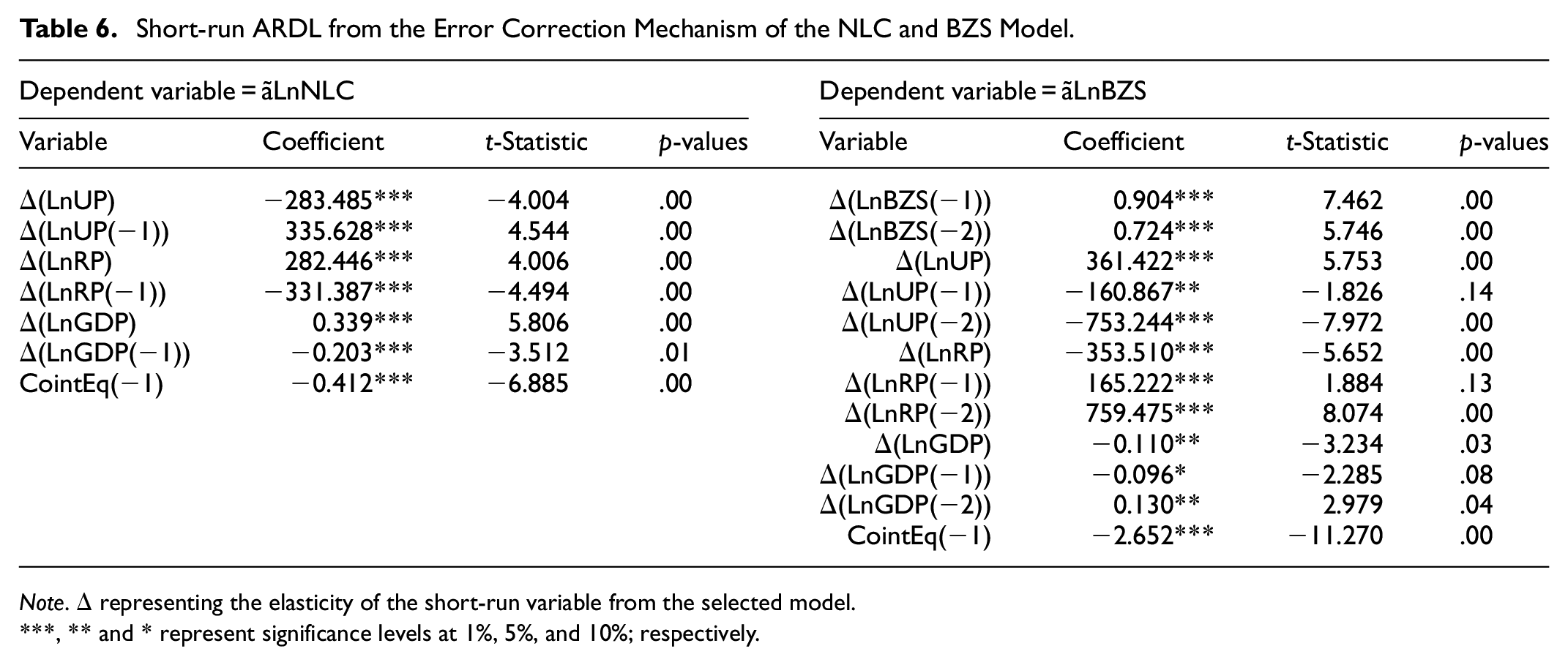
Note. Δ representing the elasticity of the short-run variable from the selected model.
, ** and * represent significance levels at 1%, 5%, and 10%; respectively.
As expected, the ECT coefficient has a negative sign and is highly significant, even at a 1% level. This indicates a long-term relationship between the dependent variable (NLC) and explanatory variables (UP, RP, and GDP). Similarly, a negative sign indicates a long-term connection between the dependent variable (BZS) and the regressor variables (UP, RP, and GDP). Our results were confirmed by (Kayani et al., 2020), who found significant long-term relationships between financial development and urban population.
Moreover, the error correction term confirms the validity of the econometric theory, which states that the ECT should be negative and statistically significant. In this case, the ECT coefficients are −0.412 and −2.652 for the NLC and the BZS, respectively. This indicates a strong and rapid adjustment process toward the equilibrium in the two models (NLC and BZS). This suggests a relatively fast speed adjustment toward the long-run equilibrium of financial development with population and economic growth.
Stability of the NLC Model
To validate the reliability of our findings, we conducted structural stability tests on the parameters of the long-run results. Following the approach suggested by Peseran and Peseran (1997), we employed the cumulative sum of recursive residuals (CUSUM) and the cumulative sum of recursive residuals of squares (CUSUMSQ) tests. These tests allowed us to assess the stability of the estimated parameters over time, providing further validation for the reliability of our results. By examining the cumulative sum of residuals and their squares, we gained insights into the consistency and robustness of the long-run relationships identified in our analysis.
Figure 3A to D display the graphical representations of the CUSUM and CUSUMSQ statistics for the NLC and BZS models. These plots serve as visual indicators of parameter constancy and model stability.

CUSUM and CUSUMSQ: (A) CUSUM tests for NLC, (B) CUSUM of Squares tests for NLC, (C) CUSUM tests for BZS, and (D) CUSUM of Squares tests for BZS.
Based on the analysis of the CUSUM and CUSUMSQ plots (blue line), we observed that most straight lines drawn at the 5% level are inside the red sprinkled lines. Specifically, the CUSUM plot remains around the zero line. Thus, the justification is that the models demonstrate parameter stability, validating the reliability of the estimated results over time. In contrast, the CUSUMSQ line for the BZS model slightly crosses the lower bound for the data points in 2017 to 2021. This indicates a potential indication of instability or deviation from the expected behavior in the estimated coefficients of the models. A small data sample can potentially contribute to crossing the CUSUMSQ line below the lower bound. Therefore, other robustness checks should be performed to validate the stability analysis results and ensure the reliability of the estimated coefficients, especially when working with limited data. We used the DOLS model for robustness checks of the validity and reliability of our models. We chose the DOLS because the estimated coefficients in DOLS provide insights into the long-term relationship between variables, allowing for the analysis of the equilibrium behavior and long-run effects of changes in the independent variables (UP, RP, and GDOP ) on the dependent variable (NLC and BZS).
Granger Causality Test
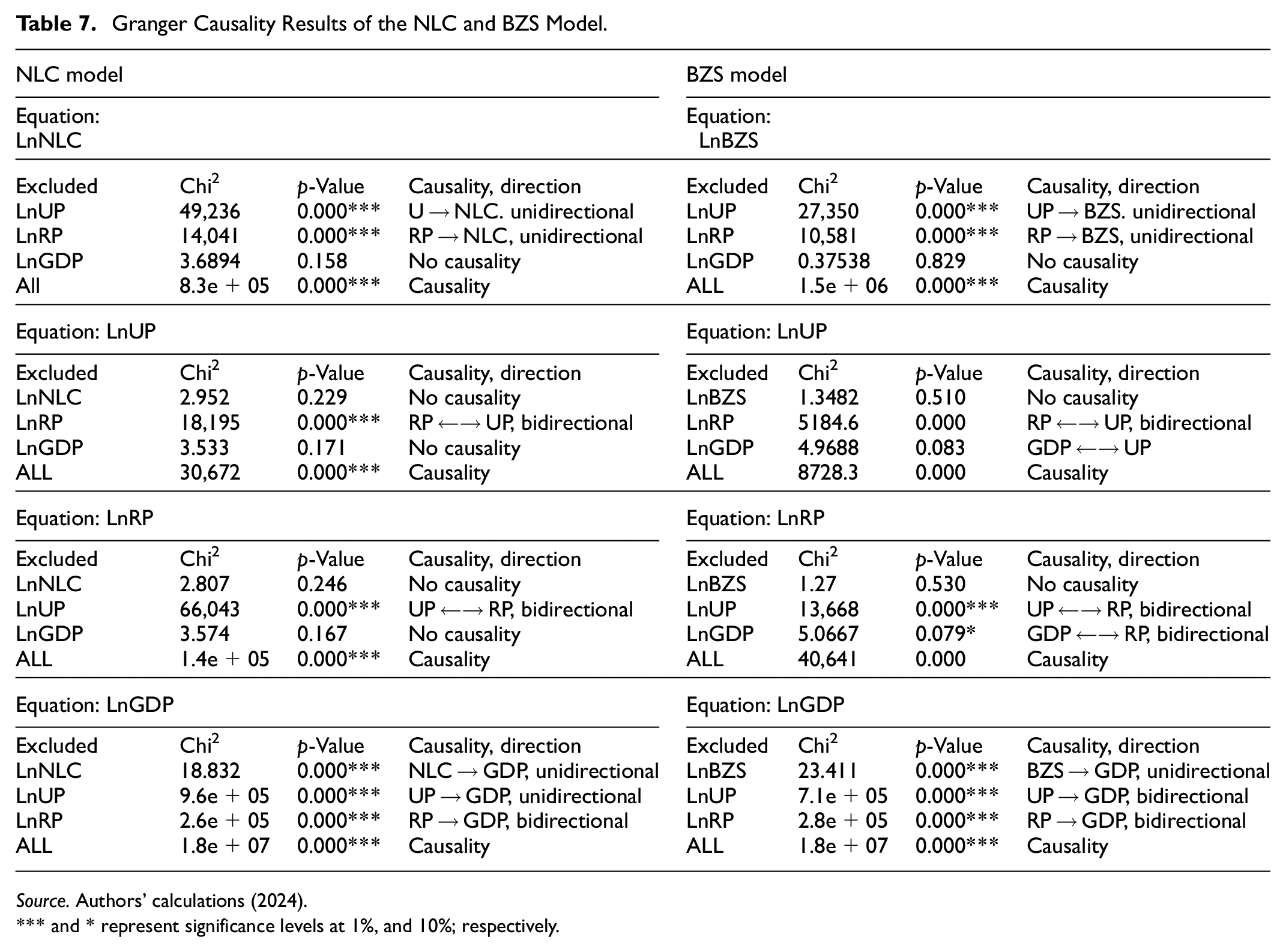
After examining the long-run relationship and cointegration between the selected variables and checking the model’s reliability, we use the Granger causality test to determine the causality between the variables. As we found cointegration among the variables, we may expect uni or bidirectional causality between the series (Table 7). UP and RP Granger caused the NLC and BZS with unidirectional causes, although the GDP did not cause the NLC or BZS. The NLC and BZS are Granger causes of the GDP. This suggests that the Granger causality test provides statistical evidence that UP and RP significantly influence NLC and BZS, whereas GDP does not have a causal effect on them. However, NLC and BZS Granger-caused GDP highlighted the financial sector’s role in driving economic growth rather than GDP influencing financial development.
Granger Causality Results of the NLC and BZS Model.
Source. Authors’ calculations (2024).
and * represent significance levels at 1%, and 10%; respectively.
We concluded a unidirectional causality running from financial development to GDP. In comparing our results with Ekanayake and Thaver (2021) and I. Khan et al. (2021), their study observed bidirectional causality running from financial development to GDP and vice versa.
DOLS Results
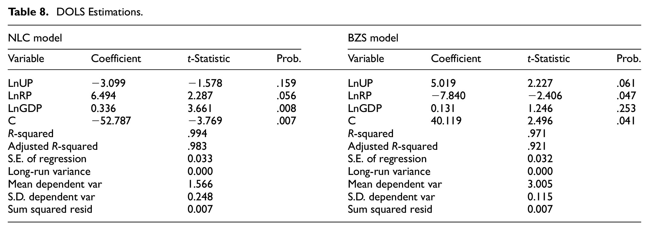
It is observed from Table 8 that robustness checks with DOLS confirm the ARDL findings. RP (at 10% level ) and GDP (at 1% level ) indicate strong significance in the NLC model. UP exerts a statistically insignificant influence on NLC, whereas GDP exerts no significant influence on BZS. While Up and RP significantly affect the BZS at 5%. Based on these results, this study concludes that the RP positively impacts NLC but negatively affects the bank’s Z-score (Table 8). Various factors, such as economic conditions, access to financial services, access to capital, regulatory environment, specific characteristics of the rural population, and market conditions, may influence this.
DOLS Estimations.
Residual Estimations
The residuals exhibit a random distribution centered around zero, indicating that the model satisfies the assumptions of linearity, independence, and constant variance. Figure 4 shows positive residuals of NLC, indicating that the model underestimated the number of listed companies, and the actual values are higher than expected. Moreover, negative residuals indicate that stricter regulations and increased compliance requirements discourage companies from choosing to go public and be listed on the stock exchange.
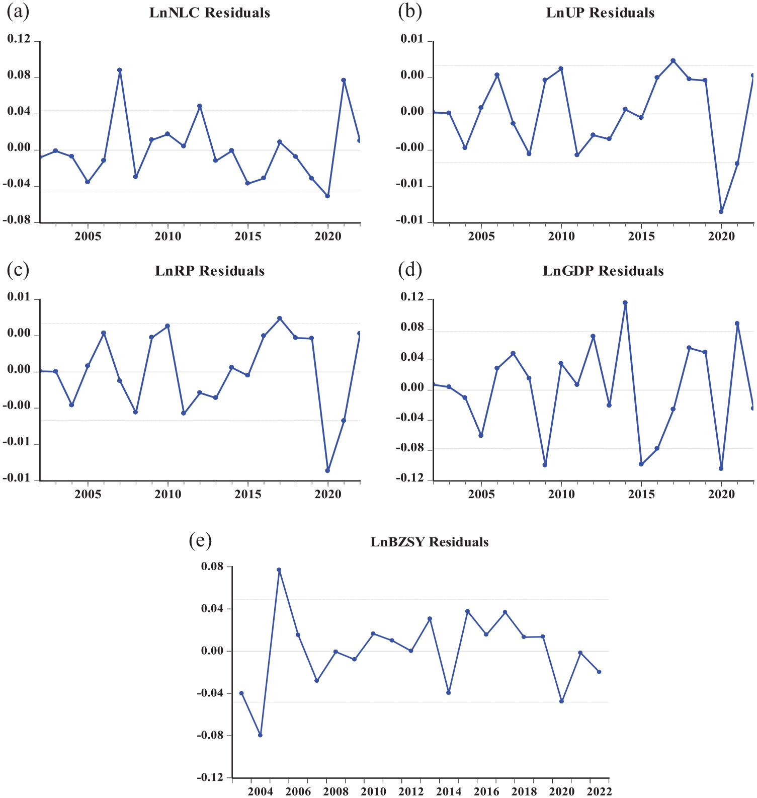
Analyzing residual plots. The graphical record illustrates the residuals for each chosen variable obtained from the model. The x-axis denotes the period, while the y-axis represents the residuals. These residuals are computed as the disparities between observed and predicted values. A solid horizontal blue line positioned at zero (acts as a reference point) for identifying deviations from the expected values. The a, b, c, d and e are the residuals subplots for NLC, UP, RP, GDP and BZSY; respectively.
Positive residuals in a bank’s Z-score indicate that the bank’s financial health is stronger than projected. This suggests a favorable performance and stability. On the other hand, negative residuals imply potential financial distress or weaker performance compared to expectations.
This means that the institution or entity may be experiencing financial difficulties or underperforming relative to expectations, which could indicate potential financial distress. Within this framework, researchers aim to detect early warning signs of financial distress (Mselmi et al., 2017), enabling investors and policymakers to implement timely interventions before conditions deteriorate further.
To fully understand the implications of these residuals, it is crucial to analyze the specific context and consider additional factors. This may obtain a more accurate interpretation of the implications of the residuals of the selected variables. This comprehensive analysis helps in recommendations based on the observed residuals and their significance to the bank’s financial health.
Conclusions and Policy Implications
Regarding many strategies and policies that have been taken to enhance revenues and reduce expenditures in Saudi Arabia, there is still a need to improve the management of financial resources and develop sustainable sources of revenue. Therefore, this study aims to investigate the most important determinants of financial development and examine to what extent population and GDP affect financial development. The study utilizes the annual time series data from 2000 to 2022. The selected variables involve the number of listed companies and bank Z-score act as financial indicators (dependent variables), urban population, rural population, and gross domestic product represent the financial development determinants (independent variables). Before starting data analysis, we used unit root tests of Dickey and Fuller (1979, 1981) and Phillips and Perron (1988) methods. We applied the ARDL bound test to detect the cointegration of the variables. We adopted the Akaike Information Criterion (AIC) to determine the appropriate values for the maximum lags of the model. The stability of the model is checked by examining the recursive method, besides diagnostic tests, and DOLS were conducted to check model reliability. Furthermore, the Granger causality approach and residual estimations were adopted.
Dickey-Fuller and Phillips–Perron unit root tests reveal that the variables are stationary at the level; however, the UP gets stationary at the first difference. Therefore, we approved applying the ARDL approach. The ARDL bounds investigated that UP, RP, and GDP significantly affect the NLC and BZS in the long run. In the short run, as expected, the ECT coefficient has a negative sign in NLC and BZS models, indicating a long-term relationship between the financial development indicators and explanatory variables. CUSUM and CUSUMSQ plots were used to gage the effectiveness of overall modeling. Also, DOLS confirmed the reliability of the ARDL models. Granger causality approved unidirectional causes between population and NLC and population and BZS. The GDP did not cause the NLC or BZS, but The NLC and BZS are Granger causes of the GDP.
Given the impact of population on financial development, we recommend that policymakers explore and consider implementing strategies to foster population growth. This may include initiatives to improve healthcare systems, increase access to education, and promote family planning programs. Likewise, governments should focus on diversifying their economies and promoting sustainable economic growth. This can be achieved by supporting various sectors, encouraging entrepreneurship, attracting foreign investments, and implementing favorable economic policies. Also, it is important to conduct further analysis and investigation to determine the reasons for the observed deviation and assess the potential implications for the financial stability of the banks under consideration.
To effectively align the impacts of urban and rural populations, along with GDP on financial development, with the broader policy implications of Saudi Arabia’s Vision 2030, we propose an integrated approach to enhance economic diversification and growth in Saudi Arabia. This can be achieved by developing policies that enhance GDP growth to drive economic diversification, focusing on improving urban and rural development to create a more balanced and flexible economy, aligning with Vision 2030 objectives. Additionally, we suggest implementing programs to improve financial literacy, entrepreneurship, and professional skills in urban and rural populations, utilizing GDP growth to invest in human capital development and empower individuals for sustainable economic participation. Furthermore, fostering public-private partnerships can facilitate collaboration among government, private sector entities, NGOs, and local communities to ensure a coordinated approach in implementing policies that address the interconnected impacts of urban and rural populations and GDP on financial development. Furthermore, proposing programs that enhance financial literacy and entrepreneurial skills in urban and rural communities aligning with Vision 2030s human capital development objectives is highly recommended.
Our study has limitations regarding the data period, choice of indicators, and generalizability, that is, the findings may be specific to the chosen period, geographical scope, and sample, making it challenging to apply them universally. These limitations highlight the need for further research to address these gaps and improve our understanding of the relationship between financial development, population, GDP, and other factors such as inflation rate, value-added, international trade, consumer index, etc.
Footnotes
Funding
The author(s) disclosed receipt of the following financial support for the research, authorship, and/or publication of this article: This research was funded by the Deanship of Scientific Research, King Faisal University, Al-Ahsa, Saudi Arabia, through financial support under the Student Researcher Track No. KFU250652.
Declaration of Conflicting Interests
The author(s) declared no potential conflicts of interest with respect to the research, authorship, and/or publication of this article.