Enhancing GDP Growth Forecasting with LSTM,GRU,and Hybrid Model: Evidence from South Korea

Abstract

This study examines the application of Long Short-Term Memory (LSTM) networks, Gated Recurrent Units (GRU) along with traditional econometric models in forecasting South Korea’s GDP growth. A hybrid framework is also developed, integrating these models through a meta-learner to capitalize on their complementary strengths. LSTM, with its ability to model nonlinear relationships and capture long-term dependencies, demonstrates accuracy improvements, especially during periods of economic volatility, such as the COVID-19 pandemic. The hybrid model further enhances forecasting performance by dynamically combining the strengths of LSTM and GRU with traditional approaches. This study provides a robust methodological contribution by uniting machine learning and econometric techniques, demonstrating their combined potential for enhancing forecasting accuracy and effectively addressing the complexities of diverse economic conditions.

Plain language summary

Enhancing economic forecasts with machine learning: A comparative study of models predicting South Korea’s GDP growth

This study examines how advanced forecasting models, including hybrid approaches that combine machine learning and traditional methods, can enhance the accuracy of predicting South Korea's economic growth. Traditional economic forecasting models, which rely on historical economic data, often face challenges in accurately capturing rapid and unexpected changes, such as those triggered by the COVID-19 pandemic. To address these limitations, our research compares several approaches: machine learning models such as Long Short-Term Memory (LSTM) and Gated Recurrent Units (GRU), traditional methods like Dynamic Factor Models (DFM) and Autoregressive (AR) models, and a hybrid model that integrates elements of both. Using metrics like Root Mean Square Error (RMSE) and Mean Absolute Error (MAE), we evaluate the performance of these models in predicting Gross Domestic Product (GDP) growth rates. Our findings demonstrate that LSTM models consistently outperform other individual models in accuracy, particularly during periods of significant economic volatility. Additionally, the hybrid model strikes a balance between the interpretability of traditional methods and the adaptability of machine learning, further improving forecasting performance. These results highlight the potential of machine learning and hybrid approaches to provide more robust and flexible tools for economic forecasting. The implications of this research are significant for policymakers and economic planners. Enhanced forecasting models can support better-informed economic policies and strategies, helping to mitigate economic instability during uncertain times. This study underscores the value of integrating machine learning with traditional methods and continually refining these models to respond to evolving economic challenges.

Introduction

Background and Motivation

Amid escalating global uncertainties, South Korea’s economic landscape is undergoing profound transformations. Geopolitical tensions and a paradigm shift toward higher interest rates, propelled by persistent inflationary pressures, exacerbate economic volatility. Although the COVID-19 pandemic has subsided, its residual effects continue to reverberate through both domestic and global economic frameworks.

South Korea’s export-driven economy, rapid technological progress, and exposure to global economic fluctuations present formidable challenges for economic forecasting. As one of the world’s most open economies, its GDP remains highly susceptible to shifts in trade dynamics, exchange rates, and geopolitical tensions, exacerbating volatility and unpredictability. External shocks, such as the U.S.-China trade war, can disproportionately disrupt industrial production and exports, leading to significant economic deviations. Domestically, structural impediments—an aging population, mounting household debt, and fluctuating consumption patterns—further complicate forecasting by shaping long-term growth trajectories and consumer behavior. These evolving dynamics necessitate adaptive forecasting models capable of capturing nonlinear and shifting economic relationships with greater precision.

South Korea’s policymakers and central bank are actively formulating strategies to mitigate economic fluctuations and enhance stability. However, the efficacy of macroeconomic and monetary policies hinges on accurate assessments of current conditions. Precise GDP forecasting, vital for informed decision-making, is often impeded by structural data collection challenges, causing delays that hinder timely economic analysis. To enhance GDP forecasting accuracy, researchers have explored leveraging monthly data to refine quarterly GDP predictions and other key macroeconomic indicators. A major breakthrough in this field is the development of mixed-frequency models, which address timing disparities in data releases, thereby improving forecast precision. Among these, the Dynamic Factor Model (DFM) has emerged as a cornerstone in nowcasting, effectively handling the complexities of mixed-frequency data (e.g., Bańbura et al., 2010; Bańbura & Modugno, 2014).

On the other hand, economic forecasting is increasingly shifting toward advanced predictive methods, particularly machine learning algorithms like Artificial Neural Networks (ANNs). These models transcend traditional limitations by capturing nonlinear relationships and efficiently handling large datasets. ANNs have demonstrated transformative capabilities across various fields, including translation, image recognition, and autonomous navigation, underscoring their versatility.

This paper aims to harness deep learning methodologies for GDP forecasting, acknowledging the unique complexities of macroeconomic systems. By integrating traditional econometric models, such as the Dynamic Factor Model (DFM), with adaptive machine learning techniques, this study seeks to enhance predictive accuracy and reliability. Beyond assessing model performance, this study develops a hybrid forecasting framework that merges theoretical econometric rigor with the flexibility of neural networks. Designed for economic forecasters and practitioners, the model features an intuitive interface, allowing for customization and adaptation to specific analytical needs. Ultimately, this research contributes to economic forecasting by improving accuracy, adaptability, and user engagement in analyzing South Korea’s economic growth patterns.

Related Literature

Machine learning has significantly impacted macroeconomic forecasting, demonstrating strong predictive capabilities compared to traditional models. However, while advances in data and algorithmic design have improved its effectiveness, there remains no definitive consensus on its superiority.

Early studies, such as Swanson and White (1997) and Biau and D’Elia (2012), demonstrated machine learning’s edge over traditional models in GDP forecasting. Later research (Jung et al., 2018; Tiffin, 2016) confirmed the effectiveness of ensemble techniques, including Random Forest and Recurrent Neural Networks. Machine learning’s role in central banking has grown, with McAdam and Warne (2020) documenting its impact on macroeconomic analysis. Medeiros et al. (2021) found Random Forest models excelled in inflation forecasting, while studies by Tkacz (2001) and others validated neural networks’ superiority over AR models.

Deep learning, particularly LSTM networks, has further refined forecasting by capturing nonlinear and temporal dependencies. Studies by Wang et al. (2023) and Alizadegan et al. (2024) confirmed LSTM’s superior accuracy in GDP and energy consumption forecasting, solidifying its role in modern predictive analytics.

Expanding upon these advancements, hybrid models that combine traditional econometric methods with deep learning techniques have emerged as a promising solution. These models effectively leverage the complementary strengths of each approach: traditional models provide interpretability and theoretical grounding, while machine learning models address nonlinear dynamics and complex interactions. For instance, Atif (2025) compared ARIMA-LSTM and ARIMA-Temporal Convolutional Network (TCN) models for long-term GDP forecasting. Their study revealed that both hybrid models achieved higher predictive accuracy than standalone ARIMA or LSTM models, with the ARIMA-TCN model delivering the best performance.

Similarly, Saleti et al. (2024) introduced an innovative hybrid model that integrates ARIMA with LSTM networks, enhanced by a moving average mechanism. This model capitalizes on ARIMA’s strength in capturing linear dependencies while utilizing LSTM’s capacity for modeling nonlinear relationships. The addition of a moving average component smooths out short-term fluctuations, making the model particularly robust in handling noisy time-series data. The study highlights the superior accuracy of this approach compared to standalone ARIMA or LSTM models, reinforcing the utility of hybrid frameworks in economic forecasting.

The relevance of hybrid approaches is also evident in financial forecasting. For instance, Alizadegan et al. (2024) conducted a comparative study on Bitcoin price forecasting using machine learning and deep learning algorithms, emphasizing the effectiveness of hybrid models in combining the interpretability of traditional methods with the complexity-capturing abilities of deep learning. This underscores the broader applicability of hybrid models in addressing forecasting challenges across various domains.

Another significant development in hybrid modeling is the meta-learner framework, which combines forecasts from multiple base models using a secondary model to produce an optimally weighted forecast. This approach aligns with ensemble learning methodologies, where weights are assigned to base model predictions based on their performance. For instance, Michańków and Kwiatkowski (2023) demonstrated the effectiveness of a hybrid model combining GARCH and GRU networks for forecasting financial volatility. Their findings showed that such hybrid models consistently produced more accurate volatility forecasts than individual models, showcasing the benefits of integrating traditional and modern approaches.

Objectives and Contributions

This study evaluates the forecasting performance of Long Short-Term Memory (LSTM), Gated Recurrent Units (GRU), Autoregressive, and Dynamic Factor Models (DFM), along with a hybrid framework that optimally combines their strengths via a meta-learner. The hybrid model integrates traditional econometric approaches (AR(1), DFM) with machine learning techniques (LSTM, GRU) to capture both linear and nonlinear patterns, enhancing forecasting accuracy, especially during economic volatility.

The adoption of hybrid models reflects advancements in economic forecasting, addressing the need for both interpretability and adaptability. Traditional econometric models offer theoretical grounding, while machine learning excels in recognizing complex patterns and adapting to evolving economic conditions. This integration provides a more robust forecasting toolkit for researchers and policymakers. Machine learning techniques, particularly LSTM and GRU, have demonstrated their ability to complement traditional methods by improving accuracy and adaptability. Leveraging large datasets and nonlinear modeling capabilities, these algorithms align with broader trends in economic forecasting. This study incorporates these methodologies into its hybrid framework to enhance predictive precision.

Applying the hybrid framework to South Korea’s GDP forecasting, especially during volatile periods like the COVID-19 pandemic, underscores its practical relevance. By combining traditional models with machine learning’s adaptability, the framework improves forecasting accuracy and responsiveness to dynamic economic shifts. LSTM and GRU further strengthen the hybrid model by capturing nonlinear relationships and adapting to sudden economic changes. These machine learning techniques complement traditional models, particularly during crises when volatility challenges conventional approaches. Overall, this hybrid framework represents a significant advancement in economic forecasting by integrating econometric models with modern machine learning. It provides a robust, adaptable solution to forecasting challenges, offering valuable insights and tools for policymakers and researchers while paving the way for future innovations in the field.

The paper is structured as follows: Section “Methodology” discusses the methodology, including the specific econometric and machine learning techniques employed. Section “ Data and Hyperparameters” provides a detailed overview of the data used and hyperparameters employed in the construction of our forecasting models. Section “Results” presents the empirical results, offering a comparative analysis of the model’s performance against established benchmarks. Finally, Section “Discussion and Conclusion” concludes with a discussion of the implications of our findings for economic forecasting and policy formulation in South Korea, and future research directions.

Methodology

Overview

The GDP forecasting model developed in this study consists of three intricately designed modules, each dedicated to a specific aspect of the forecasting process. These modules combine traditional econometric approaches with modern machine learning techniques, with the aim of improving the accuracy and reliability of economic growth predictions. Figure 1 illustrates the overall structure of the forecasting model developed in this study.

Figure 1.

The flowchart of the forecasting process.

• Module 1: Data Collection and Preprocessing

The first module serves as the foundation of the forecasting model, focusing on the meticulous collection and preprocessing of relevant economic data. This phase is crucial for ensuring the data’s quality and compatibility with the forecasting process. It involves:

• Gathering raw economic indicators and datasets from a variety of sources, including national and international databases. This step is vital for capturing a broad spectrum of factors that influence economic growth.

• Processing the collected data to make it suitable for analysis. This includes cleaning the data, handling anomalies, and making adjustments for seasonality or other cyclical factors. The goal is to standardize the datasets, enabling consistent and accurate analysis across different economic variables.

• Module 2: Missing Data Handling

In the second module, we address the challenges associated with missing values commonly found in economic datasets. Specifically, the module will focus on the following:

• Addressing the issue of missing data, which can skew analysis and lead to inaccurate forecasts. We use sophisticated methods to estimate missing values, ensuring that the dataset is complete and representative of the underlying economic conditions.

• Module 3: Deep Learning-Based Prediction

The final module is where the forecasting model comes together, using deep learning algorithms to predict future economic growth rates. This module:

• Prepares the processed and refined data from the previous modules, transforming it into a format suitable for training deep learning models. This involves structuring the data in a way that maximizes the model’s learning efficiency.

• Utilizes advanced neural network architectures, such as Recurrent Neural Networks (RNNs), which are particularly adept at handling sequential data. These models are trained on historical economic data, learning patterns and relationships that can predict future growth rates.

• Fine-tunes the model through hyperparameter optimization, searching for the best combination of parameters that enhance the model’s predictive accuracy. This step is critical for adapting the model to the nuances of economic data and ensuring that it can generalize well to unseen data.

Together, these modules form a comprehensive framework for forecasting economic growth rates, leveraging both the depth of economic theory and the breadth of machine learning capabilities. In the subsequent subsections, we provide comprehensive descriptions of the primary modules utilized throughout the analysis.

Module 1: Data Collection and Preprocessing

The forecasting model begins with data collection and preprocessing to ensure accuracy. This study uses the Bank of Korea’s Open API (https://ecos.bok.or.kr/api/#/) to extract macroeconomic indicators like GDP growth, inflation, and unemployment, ensuring data reliability.

To address nonstationary behavior, differencing removes trends while preserving patterns. Seasonal adjustments via X13-ARIMA eliminate recurring fluctuations, ensuring data reflects true economic trends. Z-score normalization standardizes variables, preventing dominance by any single factor and improving model efficiency. These preprocessing steps create a robust foundation for accurate forecasting, ensuring consistency and reliability in subsequent modeling.

Module 2: Missing Values Problem

Forecasting short-term GDP growth using mixed-frequency data faces challenges due to missing values, known as the Ragged-Edge issue. This arises from discrepancies in data availability and release schedules. While quarterly data lack monthly counterparts, monthly indicators vary in publication lags—for example, consumer confidence is released immediately, whereas unemployment and production indices have delays (1–2 months). GDP growth rates also undergo preliminary and revised releases, complicating real-time accuracy.

To address these issues, various methods have been explored. The bridge equation model averages monthly data to match quarterly frequencies but risks information loss and distortion (Diron, 2008; Golinelli & Parigi, 2007; Parigi & Schlitzer, 1995; Rünstler et al., 2009; Trehan, 1989). MIDAS (Mixed Data Sampling) retains high-frequency data richness by incorporating distributed lag polynomials into regressions (Tsui et al., 2018), avoiding simple averaging.

Recent nowcasting models integrate the Dynamic Factor Model (DFM) with the Expectation-Maximization (EM) algorithm to handle mixed-frequency data and missing values (Angelini et al., 2008; Bańbura & Modugno, 2014; Bańbura et al., 2010; Marcellino & Schumacher, 2010; Mariano & Murasawa, 2003; Mitchell et al., 2005; Proietti, 2008; Stock & Watson, 2002) . These models estimate missing values and extract key economic factors.

This study employs a DFM-EM approach, surpassing single-equation models by addressing the Ragged-Edge problem and uncovering hidden relationships among economic indicators. This method enhances short-term GDP forecasting accuracy by estimating parameters from underlying probability distributions, effectively incorporating hard-to-observe variables. See Appendix A for EM algorithm details.

The core of the Dynamic Factor Model (DFM) is captured in the following equations, providing a concise representation of the complex relationships among the observed variables, latent factors, and the idiosyncratic components:

Measurement Equation:

$$\begin{array}{c}{y}_t=\mu +\Lambda f_t+{ϵ}_t\hfill \end{array}$$

(1)

Transition Equation:

$$\begin{array}{c}{f}_t=A_1{f}_{t-1}+\dots +A_p{f}_{t-p}+u_t,u_t~i.i.d.N(0,Q)\hfill \end{array}$$

(2)

$$\begin{array}{c}{ϵ}_{\mathrm{it}}={\alpha }_i{ϵ}_{\mathrm{it}-1}+{\xi }_{\mathrm{it}}\hfill \end{array}$$

(3)

$$\begin{array}{c}{\xi }_{\mathrm{it}}~i.i.d.N(0,{\sigma }_i^2)\hfill \end{array}$$

(4)

In this framework, $y_t$ represents the vector of observed variables, $f_t$ denotes the latent factors, ${ϵ}_t$ is the vector of idiosyncratic errors, and $u_t$ captures the dynamics of the latent factors. The matrices $A_1$ to $A_p$ are the parameters modeling the relationships between the factors over time, and $\Lambda$ represents the factor loadings, which map the latent factors onto the observed variables. The EM algorithm, in this context, enables the estimation of the DFM’s parameters, even in the presence of missing data, by alternating between the expectation (E-step) and maximization (M-step), an iterative process that converges to the maximum likelihood estimates of the parameters.

Additionally, the use of principal component analysis (PCA) helps identify the key underlying factors that contribute to variations in complex datasets. PCA simplifies the process by reducing dimensionality and extracting the most pertinent information, which is then used to determine the number of significant factors. The choice of how many factors to consider is guided by established criteria such as Kaiser (1960)’s criterion and the proportion of variance explained by each factor.

The model also utilizes a state-space representation in the following form:

$$\begin{array}{c}{y}_t=\mu +Z\left(\theta \right)s_t\hfill \end{array}$$

(5)

$$\begin{array}{c}{s}_t=T\left(\theta \right)s_{t-1}+{\eta }_t\hfill \end{array}$$

(6)

where $y_t$ denotes the measurement vector, $s_t$ symbolizes the state vector incorporating both the factors $f_t$ and the idiosyncratic shocks ${ϵ}_t$ , and ${\eta }_t$ captures the state vector’s innovations. For $p=1$ , $s_t=(f{\text{'}}_t,{ϵ}_{1t},\cdots ,{ϵ}_{\mathrm{nt}})\text{'}$ .The functions $Z\left(\theta \right)$ and $T\left(\theta \right)$ map the state vector into the observed data space and define the transition of states over time, respectively. This state-space model (SSM) underlines the DFM’s ability to handle the dynamics within the macroeconomic indicators.

The DFM is designed to address the limitations of incomplete data and provides a deeper understanding of economic indicators, pushing the field of macroeconomic forecasting forward. By using the EM algorithm and SSM, this study enables a thorough analysis, leading to more timely and precise economic predictions that are essential for policy-making and economic analysis.

At the core of the model are the measurement and transition equations, which describe the evolution of economic indicators and their underlying factors over time. In our model, the measurement equation is represented by:

$$\begin{array}{c}{x}_t=\mu +\left[\Lambda I_n\right]f_t\hfill \end{array}$$

(7)

where $x_t$ is the vector of observed variables at time, $\mu$ symbolizes the intercept term, and $\Lambda$ is the matrix of factor loadings that connects the observed data to the latent factors. This equation captures the direct influence of the latent factors on the observed variables.

The transition equation describes how the latent factors and idiosyncratic terms evolve over time:

$$\begin{array}{c}\left[\begin{array}{c}{f}_t\hfill \\ \multicolumn{1}{c}{{ϵ}_t}\end{array}\right]=\left[\begin{array}{cc}{A}_1\hfill & 0\hfill \\ \multicolumn{1}{c}{0}& \mathrm{diag}({\alpha }_1,\dots ,{\alpha }_n)\hfill \end{array}\right]\left[\begin{array}{c}{f}_{t-1}\hfill \\ \multicolumn{1}{c}{{ϵ}_{t-1}}\end{array}\right]+\left[\begin{array}{c}{u}_t\hfill \\ \multicolumn{1}{c}{e_t}\end{array}\right]\hfill \end{array}$$

(8)

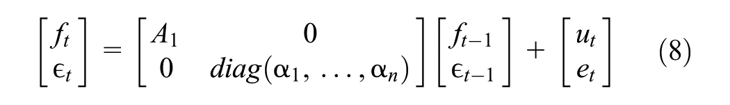
In this equation, $A_1$ represents the dynamics of the hidden factors $f_t$ , the diagonal matrix $\mathrm{diag}({\alpha }_1,\cdots ,{\alpha }_n)$ contains the autoregressive coefficients for the individual components ${ϵ}_t$ , and $u_t$ and $e_t$ stand for the innovation terms for the hidden factors and individual errors, respectively. By using the EM algorithm, this model effectively estimates the hidden states and parameters even when data is missing, leading to a more accurate forecast that considers both common and unique economic influences. The model’s ability to handle the complexities of economic data makes it a powerful tool for economists in short-term GDP forecasting and other macroeconomic analyses.

Module 3: Prediction Model with Artificial Neural Networks

Artificial Neural Networks (ANNs) play a crucial role in economic forecasting, offering strong predictive capabilities. This study employs advanced ANN-based algorithms to analyze complex economic indicators and time series data, forming the core of our predictive model. We focus on multilayer perceptrons (MLPs), recurrent neural networks (RNNs), long short-term memory (LSTM) units, and gated recurrent units (GRUs) for macroeconomic forecasting.

ANNs excel at modeling nonlinear relationships, surpassing traditional methods. MLPs capture complex interactions, while RNNs introduce temporal continuity. LSTMs address short-term memory limitations, enabling long-term pattern recognition, and GRUs offer a more efficient alternative, balancing computational efficiency and accuracy. This section details the architecture and implementation of ANN-based algorithms for forecasting South Korea’s economic trajectory, ensuring adaptability in an evolving economic landscape.

Overview of Artificial Neural Networks

The multilayer perceptron (MLP) is a fundamental artificial neural network (ANN) model that captures complex variable relationships more effectively than traditional linear econometric models. It consists of input, hidden, and output layers, as shown in Figure 2.

Figure 2.

The structure of a multilayer perceptron.

The input layer consists of neurons that receive observed values of predictive variables. These values are weighted and transformed into outputs through an activation function. For example, if the first hidden layer has four nodes, its weighted sum is defined in equation (9), and the activation function produces outputs as shown in equation (10).

$$\begin{array}{c}\multicolumn{1}{c}{z=(z_1,z_2,z_3,z_4)}\\ \multicolumn{1}{c}{=(\sum _{i=1}^d{w}_i^{\left(1\right)}{x}_i,\sum _{i=1}^d{w}_i^{\left(2\right)}{x}_i,\sum _{i=1}^d{w}_i^{\left(3\right)}{x}_i,\sum _{i=1}^d{w}_i^{\left(4\right)}{x}_i)}\end{array}$$

(9)

$$y^1=f\left(z\right)=(f\left(z_1\right),f\left(z_2\right),f\left(z_3\right),f\left(z_4\right))$$

(10)

The initial hidden layer’s outputs serve as inputs for subsequent layers in a feedforward process. MLP learns optimal weights through training, typically using the Backpropagation Through Time (BPTT) algorithm (Hecht-Nielsen, 1992). However, MLP does not account for temporal dependencies in time series data, limiting its predictive accuracy. Time series data are sequential, with current values influenced by past observations, requiring models that capture these relationships rather than treating inputs as independent.

Recurrent Neural Network

The recurrent neural network (RNN) improves upon the multilayer perceptron (MLP) for time series prediction by incorporating previous timesteps as inputs for future predictions, as shown in Figure 3.

Figure 3.

The structure of a RNN.

RNNs use previous timestep outputs as inputs for the current step, adding weight parameters (equation 11). They incorporate a memory cell that stores past information. Elman (1990) described how state variables, influenced by inputs and bias terms, are processed through an activation function (equation 12).

$$\begin{array}{c}\multicolumn{1}{c}{y_t=\varphi (W_x{x}_t+W_y{y}_{t-1}+b)}\end{array}$$

(11)

$$\begin{array}{l}{h}_t={\sigma }_h\left(W_{hx}{x}_t+U_{hh}{h}_{t-1}+b_h\right)\\ y_t={\sigma }_y\left(W_{hy}{h}_t+b_y\right)\end{array}$$

(12)

where $W_h$ , $W_y$ , and $U_h$ represent the weights matrices, $b$ is the bias term, and $\sigma$ denotes the activation function.

RNNs capture short-term patterns but struggle with long-term dependencies due to short memory. They process sequences by incorporating past outputs, making them effective for tasks like speech and handwriting recognition. However, as the gap between events grows, the vanishing gradient problem weakens the influence of early inputs during training. This limits RNNs' ability to recognize long-term patterns, requiring alternative architectures like long short-term memory (LSTM) networks and gated recurrent units (GRUs), which retain information and mitigate gradient loss.

Long Short-Term Memory Algorithm

The long short-term memory (LSTM) algorithm, developed by Hochreiter and Schmidhuber (1997), overcomes RNNs’ short memory limitations and improves model efficiency. Each LSTM cell has four layers: the main layer, forget gate, input gate, and output gate. The main layer processes the current input $x_t$ and previous hidden state h_t-1. The forget gate controls retained information, the input gate manages new data flow, and the output gate applies the tanh function and sigmoid activation to produce $h_t$ for the next timestep (Figure 4).

Figure 4.

The structure of a LSTM network.

The mathematical structure of the LSTM model is outlined in equation (13), incorporating weight matrices, logistic functions, and bias terms. However, LSTMs can suffer from slow learning and overfitting due to their numerous parameters. Regularization via dropout helps prevent overfitting by randomly deactivating connections during training, improving generalization. However, in LSTMs, dropout can be challenging to apply, as indiscriminate use may disrupt long-term dependencies, leading to performance issues, unstable training, and reduced effectiveness in learning long sequences.

$$\begin{array}{cc}\multicolumn{1}{c}{i_t}& =\sigma (W_{\mathrm{xi}}{x}_t+W_{\mathrm{hi}}{h}_{t-1}+b_i),\hfill \\ \multicolumn{1}{c}{f_t}& =\sigma (W_{\mathrm{xf}}{x}_t+W_{\mathrm{hf}}{h}_{t-1}+b_f),\hfill \\ \multicolumn{1}{c}{o_t}& =\sigma (W_{\mathrm{xo}}{x}_t+W_{\mathrm{ho}}{h}_{t-1}+b_o),\hfill \\ \multicolumn{1}{c}{g_t}& =\tanh (W_{\mathrm{xg}}{x}_t+W_{\mathrm{hg}}{h}_{t-1}+b_g),\hfill \\ \multicolumn{1}{c}{c_t}& =f_t°c_{t-1}+i_t°g_t,\hfill \\ \multicolumn{1}{c}{y_t}& =h_t=o_t°\tanh \left(c_t\right),\hfill \end{array}$$

(13)

where ° denotes the element-wise multiplication operator, $W$ represents weight matrices, $\sigma$ is the sigmoid function, and $b$ denotes the bias term for each layer.

Gated Recurrent Unit Algorithm

The gated recurrent unit (GRU) simplifies LSTM by using fewer parameters and a single state variable ${\mathrm{h}}_{\mathrm{t}}$ . Unlike LSTM’s two memory cells, GRU merges the forget and input gates into an update gate, which regulates information retention or removal (Figures 5 and 6).

Figure 5.

RNN, LSTM and GRU.

Figure 6.

The basic structure of a GRU.

The GRU lacks an output gate, allowing the full past information vector to be used at each timestep, while a separate gate controls which parts are retained. This design balances information retention and updates. In LSTMs, the forget gate regulates how much past information from ${\mathrm{h}}_{\mathrm{t}-1}$ and ${\mathrm{x}}_{\mathrm{t}}$ is retained or discarded, using a sigmoid activation function that outputs values between 0 and 1, denoted as ${\mathrm{r}}_{\mathrm{t}}$

$$\begin{array}{c}{r}_t=\sigma (W_{\mathrm{rx}}{x}_t+W_{\mathrm{rh}}{h}_{t-1}+b_r)\hfill \end{array}$$

(14)

where $W_{\mathrm{rx}}$ and $W_{\mathrm{rh}}$ are weight matrices for the input and the recurrent connection, respectively, and $b_r$ is the bias. Values close to 0 indicate that the gate is forgetting more of the previous state, while values close to 1 suggest that more of the previous state is being retained.

The update gate in a GRU architecture is crucial for balancing old and new information. Denoted by $z_t$ , it determines how much of the previous hidden state $h_{t-1}$ should be carried over to the next state. The GRU also incorporates a reset gate to help the network forget irrelevant past information before combining it with new input. Here’s the mathematical representation of these mechanisms:

$$\begin{array}{cc}\multicolumn{1}{c}{z_t}& =\sigma (W_{\mathrm{zx}}{x}_t+W_{\mathrm{zh}}{h}_{t-1}+b_z)\hfill \\ \multicolumn{1}{c}{r_t}& =\sigma (W_{\mathrm{rx}}{x}_t+W_{\mathrm{rh}}{h}_{t-1}+b_r)\hfill \\ \multicolumn{1}{c}{{\tilde{h}}_t}& =\tanh (W_x{x}_t+W_r(r_t°h_{t-1})+b)\hfill \\ \multicolumn{1}{c}{h_t}& =(1-z_t)°h_{t-1}+z_t°{\tilde{h}}_t\hfill \end{array}$$

(15)

where $\sigma$ represents the sigmoid function which outputs values between 0 and 1, facilitating the gates’ decisions to either pass or modify data. The weights $W_{\mathrm{zx}}$ , $W_{\mathrm{zh}}$ , $W_{\mathrm{rx}}$ , $W_{\mathrm{rh}}$ , $W_x$ , and $W_r$ correspond to the input and recurrent connections for each gate and the candidate state. The biases $b_z$ , $b_r$ , and $b$ adjust the output alongside the recurrent network dynamics. This configuration allows the GRU to make adaptive decisions over each timestep, enhancing its ability to handle problems involving sequences where the importance of information varies over time.

This study employs LSTM and GRU models to forecast South Korea’s GDP growth, leveraging their ability to handle sequential data and long-term dependencies. These architectures effectively manage time-series data, capturing complex economic patterns and past influences. Their application provides valuable insights into South Korea’s future economic trajectory.

This study selects LSTM and GRU models for their effectiveness in handling sequential economic data. Traditional econometric models struggle with nonlinear relationships and long-range dependencies, making LSTMs and GRUs better suited for economic forecasting. LSTMs capture long-term dependencies using memory cells and gating mechanisms, making them ideal for datasets with complex temporal patterns. Their ability to retain contextual information enhances forecasting accuracy over extended horizons.

GRUs, with a simpler architecture and fewer parameters, reduce computational burden while maintaining strong performance. Their efficiency makes them preferable for tasks with less complex data patterns or shorter-term dependencies. By combining LSTMs’ memory management with GRUs’ computational efficiency, this study balances accuracy and resource constraints, offering insights into their trade-offs in economic forecasting.

Hybrid Model: Meta Learner

This paper also develops a meta-learner hybrid model using a linear regression framework. It combines forecasts from four base models, assigning optimal weights through ordinary least squares (OLS) regression to minimize mean squared error (MSE) and improve predictive accuracy.

The input features to the meta-learner are the one-step-ahead forecasts from the base models:

$$\begin{array}{c}X=\left[\begin{array}{c}{y}_{\mathrm{LSTM}}\hfill \\ \multicolumn{1}{c}{y_{\mathrm{GRU}}}\\ \multicolumn{1}{c}{y_{\mathrm{DFM}}}\\ \multicolumn{1}{c}{y_{\mathrm{AR}\left(1\right)}}\end{array}\right]\hfill \end{array}$$

(16)

Here:

• Y _LSTM is the forecast from the Long Short-Term Memory (LSTM) model.

• Y _GRU is the forecast from the Gated Recurrent Unit (GRU) model.

• Y _DFM is the forecast from the Dynamic Factor Model (DFM), which captures co-movements across multiple economic indicators.

• Y _AR(1) is the forecast from a simple autoregressive model, which serves as a benchmark for capturing linear relationships.

The target variable, $Y$ , is the actual observed value of the economic indicator (e.g., GDP growth) at the corresponding forecast horizon. For one-step-ahead forecasts, the meta-learner estimates the following relationship:

$$Y_t={\beta }_0+{\beta }_1{y}_{\mathrm{LSTM},t}+{\beta }_2{y}_{\mathrm{GRU},t}+{\beta }_3{y}_{\mathrm{DFM},t}+{\beta }_4{y}_{\mathrm{AR}\left(1\right),t}+{ϵ}_t$$

(17)

where:

• β₀, β₁, β₂, β₃, β₄ are the regression coefficients (weights) learned by the meta-learner.

• ϵ_t is the error term.

The weights ( ${\beta }_1,{\beta }_2,{\beta }_3,{\beta }_4$ ) are optimized using OLS regression:

$$\begin{array}{c}\hat{\beta }=\arg \underset{\beta }{\min }\sum _{t=1}^T{(Y_t-{\beta }_0-\sum _{i=1}^4{\beta }_i{y}_{\mathrm{mode}{l}_i,t})}^2\hfill \end{array}$$

(18)

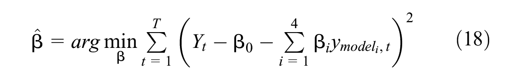
This optimization ensures that the meta-learner minimizes the residual error between the combined forecast and the actual observed value over the training period. The hybrid model capitalizes on the unique strengths of each base model:

• LSTM and GRU excel in capturing nonlinear patterns and long-term dependencies in time series data.

• DFM effectively aggregates information from multiple economic indicators, capturing co-movements and broader macroeconomic trends.

• AR(1) provides a robust baseline for linear relationships and short-term dynamics.

The meta-learner assigns data-driven weights to each base model, reflecting their relative importance and accuracy. This approach improves adaptability and ensures that the combined forecast is tailored to the specific characteristics of the data.

By combining forecasts from diverse models, the meta-learner mitigates the risk of model-specific biases and overfitting. The hybrid model averages out idiosyncratic errors while preserving the predictive strengths of individual approaches.

Data and Hyperparameters

Overview

This study utilizes a dataset from 2001 to 2021, covering both normal conditions and economic crises, including COVID-19. Data is sourced from the Bank of Korea’s economic database, with explanatory variables selected based on established research (Kim & Kang, 2020; Oh, 2022). Table 1 details transformations: the “DIFF” column indicates whether log differencing was applied, while the “LAG” column specifies data publication delays—two months for quarterly data and varying lags for monthly data. The “FREQ” column denotes publication frequency, with “M” indicating monthly data.

Table 1.

List of Variables.

Variable	Description	LAG	DIFF	FREQ
GDP	Gross Domestic Product Growth Rate	2	0	Q
PROD	Industrial Production Index, Total (Excluding Agriculture), Seasonally Adjusted	2	1	M
PRODMAN	Industrial Production Index, Manufacturing (Seasonally Adjusted)	2	1	M
PRODSER	Industrial Production Index, Services (Seasonally Adjusted)	2	1	M
PRODMIN	Mining Production Index (Seasonally Adjusted)	2	1	M
MAFSHIP	Manufacturing Shipments Index (Seasonally Adjusted)	2	1	M
MAFINVEN	Manufacturing Inventory Index (Seasonally Adjusted)	2	1	M
INTENSITY	Manufacturing Utilization Index (Seasonally Adjusted)	2	0	M
LEADINDEX	Leading Economic Index (Seasonally Adjusted)	2	0	M
COINDEX	Coincident Economic Index (Seasonally Adjusted)	2	0	M
RETAILSALES	Retail Sales Index (Seasonally Adjusted)	2	1	M
RETAILSALESD	Retail Sales Index, Durables (Seasonally Adjusted)	2	1	M
RETAILSALESND	Retail Sales Index, Non-Durables (Seasonally Adjusted)	2	1	M
INVESTIND	Investment Index (Seasonally Adjusted)	2	1	M
CONSAMT	Construction Output, Constant (Seasonally Adjusted)	2	0	M
CPI	Consumer Price Index (Total)	1	1	M
PPI	Producer Price Index (Total)	1	1	M
IPI	Import Price Index (Total)	1	1	M
EXPI	Export Price Index	1	1	M
CPI_EXAGRI	Consumer Price Index (Excluding Agriculture and Petroleum)	1	1	M
CPI_EXFOODS	Consumer Price Index (Excluding Food and Energy)	1	1	M
EMP_NUM	Number of Employed (Seasonally Adjusted)	1	1	M
UEMPR	Unemployment Rate (Seasonally Adjusted)	1	0	M
EMPR	Employment Rate (Seasonally Adjusted)	1	0	M
ECONPART_RATE	Economic Participation Rate (Seasonally Adjusted)	1	0	M
M1END	M1 Money Supply (End of Period, Seasonally Adjusted)	2	1	M
M2END	M2 Money Supply (End of Period, Seasonally Adjusted)	2	1	M
LFEND	Liquid Funds, (End of Period, Seasonally Adjusted)	2	1	M
EXP	Export Value (Customs Basis)	1	1	M
IMP	Import Value (Customs Basis)	1	1	M
BSI_SALES	All Industry Sales BSI (Actual)	0	0	M
BSI_ENV	All Industry Business Conditions BSI (Actual)	0	0	M
BSI_MAF_EX	Manufacturing Export BSI	0	0	M
BSI_MAF_INTENSITY	Manufacturing Utilization BSI	0	0	M
BSI_MAF_DOMESTIC	Manufacturing Domestic Sales BSI	0	0	M
BSI_MAF_ENV	Manufacturing Business Conditions BSI	0	0	M
SENT	Economic Sentiment Index (CSI + BSI) (Seasonally Adjusted)	0	0	M

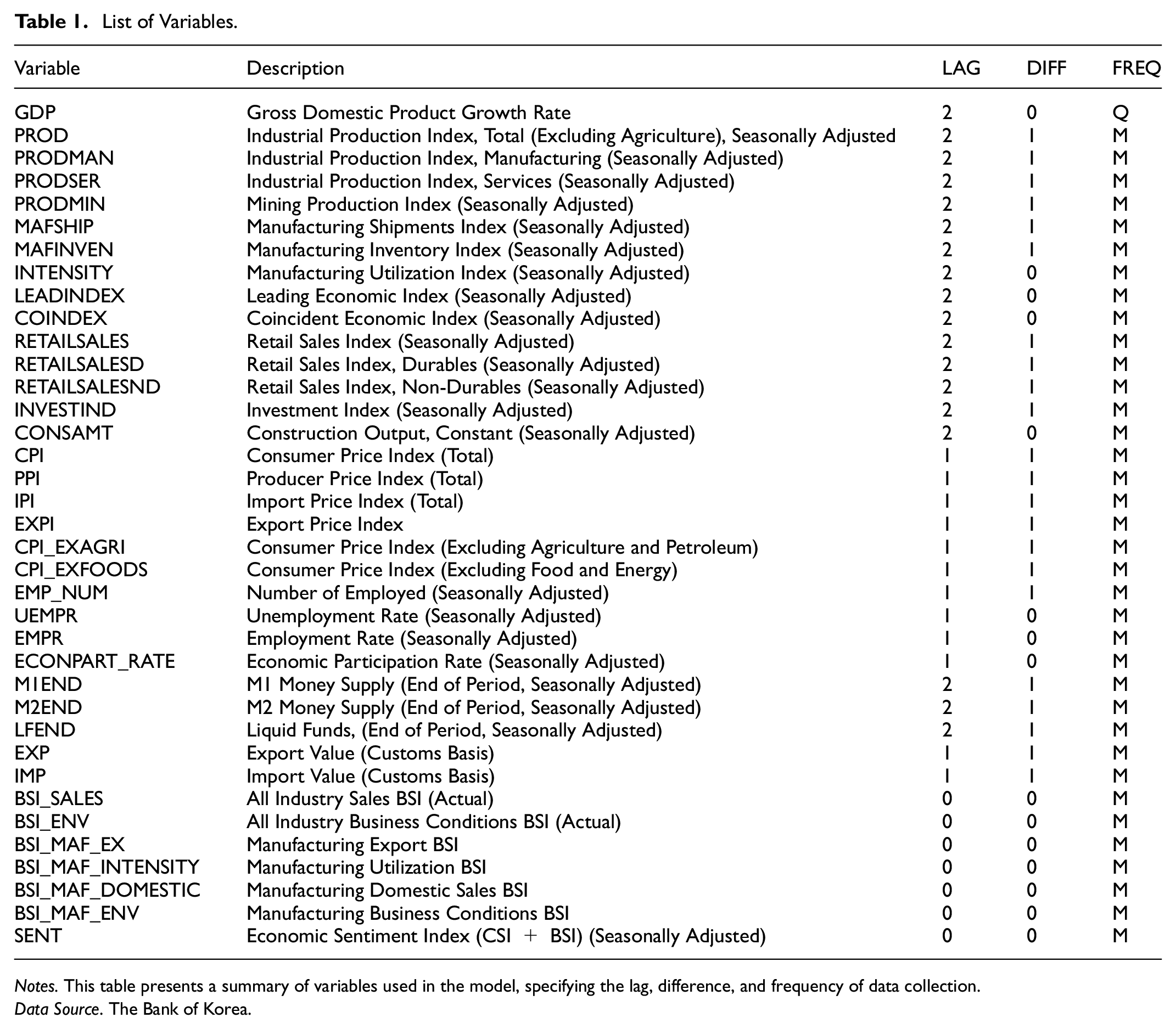
Notes. This table presents a summary of variables used in the model, specifying the lag, difference, and frequency of data collection.

Data Source. The Bank of Korea.

Survey-based indices such as the Consumer Confidence Index (CSI) and Business Survey Index (BSI) provide early economic insights but face criticism for limited sample sizes and potential disconnect from actual consumer behavior. For instance, despite a CSI decline in early 2020, consumer spending remained inconsistent with expectations, as South Korea recorded its lowest quarterly growth rate (−3%) in a decade. Seasonally adjusted data is used, and when unavailable, adjustments are made using the X-11 ARIMA model, which decomposes time series into trend, seasonal, and irregular components for accurate seasonal adjustment.

Training Data Structure and Forecasting Process

In recurrent neural networks (RNNs) like long short-term memory (LSTM) and gated recurrent unit (GRU) networks, selecting the appropriate historical data window, or timesteps, is crucial for accurate predictions. A larger timestep allows the model to capture long-term economic patterns. The network's output at each timestep $\mathrm{t}-1$ serves as input for $\mathrm{t}$ .

For example, when forecasting June 2020, the model uses explanatory variables from the past 10 months, up to March 2020, to ensure both short-term and long-term trends are incorporated. The optimal timestep length was determined using a grid search, enhancing forecasting accuracy.

Once trained, the model predicts GDP growth using input variables for the next quarter. The accuracy of predictions depends on the availability of complete data, which can be affected by the ragged-edge issue—missing values in the target quarter. To address this, missing data is estimated using the Dynamic Factor Model (DFM), as detailed in Module 2. If explanatory variables are incomplete (e.g., forecasting at the end of May 2020 for June 2020), DFM imputes missing values to ensure consistent forecasting.

Hyperparameters Setting

The forecasting model optimizes key hyperparameters, including the number of hidden layers, units per layer, and learning rate, which controls parameter adjustments during training. Activation functions and regularization techniques like dropout help prevent overfitting.

A grid search was conducted to evaluate hyperparameter combinations from January 2001 to December 2020. The best configuration was selected based on the lowest root-mean-squared-error (RMSE) from validation data, which comprised 25% of the dataset. See Appendix B for details on hyperparameter optimization.

The grid search tested a range of hyperparameters, including:

• Number of hidden layers (H): $H=\{1,2,3,4,5\}$

• Number of units per layer (U): $U=\{5,6,\dots ,100\}$

• Learning rate (L): $L=\{0.1,0.01,0.001,0.0001\}$

• Activation functions (F): $\mathrm{ReLU}$ , $\tanh$ , $\mathrm{sigmoid}$

• Dropout rate (D): D = {0.0,0.1,...,0.4}

For specific values for hyperparameters used, refer to Table 2.

Table 2.

LSTM and GRU Model Hyperparameters.

Hyperparameter	LSTM	GRU
Number of layers	2	2
First layer units	8	10
First layer activation function	sigmoid	sigmoid
First layer dropout rate	0.2	0.4
Second layer units	21	75
Second layer activation function	sigmoid	sigmoid
Second layer dropout rate	0.4	0.4
Learning rate	0.1	0.1

Note. Dropout rates for LSTM and GRU models are optimized based on the specific architectural requirements of each model. Learning rates were selected to balance convergence speed and training stability. Refer to Appendix C for details on regularization techniques to mitigate overfitting.

Comparative Forecasting Performance

Benchmark Forecasting Models

This study evaluates the predictive accuracy of LSTM and GRU models against traditional benchmarks for GDP growth forecasting under different data availability conditions. Benchmark models include the autoregressive (AR) model, which uses quarterly GDP growth data with a lag order of 1 to balance simplicity and predictive power.

Since prior-quarter GDP may be unavailable early in the quarter, forecasts for the next quarter are used. The dynamic factor model (DFM) is also employed as a benchmark, maintaining the same factor loading structures as the ANN-based models.

Out-of-Sample Forecasting

When evaluating the accuracy of out-of-sample forecasts, this study uses two widely recognized metrics: Root Mean Squared Error (RMSE) and Mean Absolute Error (MAE). These metrics are crucial for assessing the predictive performance of economic forecasting models.

The RMSE is calculated using the formula:

$$\begin{array}{c}\mathrm{RMSE}=\sqrt{\frac{1}{T}\sum _{t=1}^T{({\hat{y}}_t-y_t)}^2}\hfill \end{array}$$

(19)

where ${\hat{y}}_t$ represents the predicted values, $y_t$ denotes the actual values, and $T$ is the total number of observations.

Similarly, the MAE is defined as:

$$\begin{array}{c}\mathrm{MAE}=\frac{1}{T}\sum _{t=1}^T|{\hat{y}}_t-y_t|\hfill \end{array}$$

(20)

This study evaluates forecasting accuracy using root mean squared error (RMSE) and mean absolute error (MAE) over an out-of-sample period from January 2015 to December 2020, examining how accuracy varies with data availability at different points within a quarter.

Two forecasting methods are used: recursive forecasts (RF), which expand training data over time, and rolling window forecasts (RWF), which maintain a fixed sample size. Forecasting accuracy depends on time series characteristics, particularly stationarity. Prior studies (Choi & Han, 2014; Swanson & White, 1997; Tashman, 2000) suggest that RWF may improve performance. This study compares both methods to assess their effectiveness in practical economic forecasting, contributing to better decision-making in economic analysis and policy formulation.

Results

Forecasting Results Excluding the Pandemic Periods

This section evaluates GDP growth forecasting models using root mean square error (RMSE) and mean absolute error (MAE) (Tables 3 and 4). The analysis highlights significant differences in model performance, particularly between LSTM and GRU models, assessed through recursive and rolling window forecasting methods.

Table 3.

RMSE by Forecasting Method and Timing: Excluding Pandemic Periods.

Timing	Forecast Horizon	Recursive Forecasting				Rolling-Window Forecasting
		GRU	LSTM	DFM	AR(1)	GRU	LSTM	DFM	AR(1)
	$y\left(t\right)$	0.6069**	0.4767	0.5416	0.5124	0.5567	0.4784	0.5222	0.4912
Beginning	$y(t+1)$	0.7126*	0.6411**	0.6396	0.7299	0.6444	0.6098**	0.6278	0.6944
	$y(t+2)$	1.0745*	1.0551	1.0301	1.1408	0.9937	1.0078	1.0005	1.1010
	$y(t+3)$	1.1628	1.1098**	1.0995	1.1771	1.1144	1.0822**	1.0835	1.1464
Middle	$y\left(t\right)$	0.5758*	0.4665	0.3926	0.5124	0.5109	0.4558	0.4005	0.4912
	$y(t+1)$	0.6983	0.6441**	0.6468	0.7299	0.6567	0.6424**	0.6394	0.6944
	$y(t+2)$	1.0743*	1.0541	1.0191	1.1408	1.0164	1.0273	0.9879	1.1010
	$y(t+3)$	1.1611	1.1098**	1.1086	1.1771	1.0993	1.1095	1.1095	1.1446
Ending	$y\left(t\right)$	0.5695	0.4834**	0.4977	0.5737	0.5485	0.4921	0.4823	0.5401
	$y(t+1)$	0.7172	0.6445**	0.6673	0.7115	0.6604	0.6265	0.6697	0.6863
	$y(t+2)$	1.0527	1.0438	1.0151	1.1376	0.9943	0.9828	0.9818	1.0993
	$y(t+3)$	1.1532*	1.1116**	1.1165	1.1776	1.0948	1.0945	1.0941	1.1470
All months	$y\left(t\right)$	0.5843*	0.4756**	0.4814	0.5336	0.5391*	0.4757	0.4710	0.5080
	$y(t+1)$	0.7094	0.6432**	0.6514	0.7238	0.6539	0.6264	0.6459	0.6917
	$y(t+2)$	1.0672*	1.0510	1.0214	1.1398	1.0015	1.0616	0.9901	1.1005
	$y(t+3)$	1.1590	1.1104	1.1082	1.1773	1.1028	1.0840	1.0919	1.1466

Notes. The table presents Root Mean Squared Error (RMSE) values for different forecasting methods across varying time periods (beginning, middle, end, and all months of the quarter) and forecast horizons. Recursive forecasting and rolling-window forecasting methods are evaluated for models including GRU, LSTM, DFM, and AR(1). Significance at the 10% level based on the Diebold and Mariano (1995) test is indicated as follows: * for squared forecast error comparisons against the DFM model, ** for comparisons against the AR(1) model.

Table 4.

MAE by Forecasting Method and Timing: Excluding the Pandemic Periods.

Timing	Forecast Horizon	Recursive Forecasting				Rolling-Window Forecasting
		GRU	LSTM	DFM	AR(1)	GRU	LSTM	DFM	AR(1)
	$y\left(t\right)$	0.5146**	0.3776	0.4151	0.4106	0.4662	0.3745	0.4057	0.4028
Beginning	$y(t+1)$	0.5456*	0.4620***	0.4759	0.5318	0.4919	0.4466***	0.4962	0.5115
	$y(t+2)$	0.6969*	0.6456**	0.6280	0.7063	0.6230**	0.6323**	0.6227	0.6810
	$y(t+3)$	0.7762	0.6920**	0.7204	0.7554	0.7866	0.6761**	0.7114	0.7350
Middle	$y\left(t\right)$	0.4844*	0.3716	0.3269	0.4106	0.3992	0.3562	0.3451	0.4028
	$y(t+1)$	0.5356	0.4672**	0.4806	0.5318	0.4939	0.4691**	0.4918	0.5115
	$y(t+2)$	0.7099*	0.6452**	0.6075	0.7063	0.6503*	0.6305**	0.5953	0.6810
	$y(t+3)$	0.7606	0.6855**	0.7006	0.7554	0.7272	0.6866***	0.7173	0.7350
Ending	$y\left(t\right)$	0.4680	0.3762**	0.3742	0.4838	0.4454	0.3745**	0.3614	0.4545
	$y(t+1)$	0.5695**	0.4669**	0.5013	0.5128	0.4915	0.4587***	0.5307	0.5025
	$y(t+2)$	0.6645*	0.6339***	0.6060	0.7028	0.6242	0.6081***	0.5869	0.6770
	$y(t+3)$	0.7796*	0.6955	0.7174	0.7557	0.7165	0.7053	0.7319	0.7368
All months	$y\left(t\right)$	0.4890***	0.3751**	0.3721	0.4350	0.4369*	0.3684**	0.3707	0.4201
	$y(t+1)$	0.5502	0.4654	0.4859	0.5255	0.4924	0.4581	0.5062	0.5085
	$y(t+2)$	0.6904*	0.6416*	0.6138	0.7051	0.6325	0.6236	0.6016	0.6797
	$y(t+3)$	0.7721***	0.6910**	0.7128	0.7555	0.7375	0.6833***	0.7202	0.7356

Notes: The table presents Mean Absolute Error (MAE) for different forecasting methods across varying time periods (beginning, middle, end, and all months of the quarter) and forecast horizons. Recursive forecasting and rolling-window forecasting methods are evaluated for models including GRU, LSTM, DFM, and AR(1). Significance at the 10% level based on the Diebold and Mariano (1995) test is indicated as follows: * for squared forecast error comparisons against the DFM model, ** for comparisons against the AR(1) model, and *** for comparisons against both the DFM and AR(1) models.

LSTM consistently outperformed other models, achieving a lower RMSE of 0.48 compared to GRU’s 0.58. The Diebold & Mariano (1995) test confirmed significant differences between GRU and the dynamic factor model (DFM), with GRU generally underperforming. However, no notable accuracy gap was found between LSTM and DFM, suggesting comparable performance across different time frames. As the forecast horizon extended, RMSE increased for all models, with prediction errors growing over time. Even three quarters ahead, RMSE values approached those of AR(1) models, indicating performance convergence. However, LSTM consistently maintained an accuracy advantage over AR(1) in both short- and long-term forecasts.

Forecast errors varied across the quarter but showed no significant differences in LSTM and GRU models. However, both models exhibited increased errors toward the quarter’s end, suggesting potential instability or sensitivity to data availability. LSTM consistently demonstrated superior adaptability, particularly in mid- and late-quarter periods, maintaining lower MAE values. The GRU model had higher MAE in recursive forecasts but improved significantly in rolling window setups, especially early in the quarter. This suggests GRU benefits from frequent updates to its forecasting window, aligning with Chung et al. (2014), who noted GRU’s advantage in handling smaller datasets with frequent data changes.

Traditional models like DFM and AR(1), while effective in stable periods, recorded higher MAE values as the quarter progressed, reflecting their difficulty in capturing late-quarter economic nuances. These findings align with Stock and Watson (2002), who highlighted challenges faced by traditional econometric models in volatile conditions. Forecast errors increased with longer horizons, reinforcing the difficulty of long-term economic forecasting, consistent with Tashman (2000), who noted declining accuracy as uncertainty accumulates. The Diebold and Mariano (1995) test also confirmed GRU’s underperformance relative to DFM, underscoring the need for model refinement or hybrid approaches integrating machine learning techniques.

Despite these challenges, LSTM consistently outperformed other models across both recursive and rolling window forecasts, confirming its superior ability to capture complex patterns in economic data (Gers et al., 2000). The findings underscore the importance of model selection based on forecasting timeframe and economic conditions. LSTM and GRU models showed clear advantages over DFM and AR(1) in handling economic fluctuations. LSTM, in particular, demonstrated strong resilience, especially during mid- and late-quarter forecasts.

Forecasting Results including the Pandemic Periods

This section evaluates the performance of various forecasting models during the COVID-19 pandemic (Tables 5 and 6). The economic disruptions posed unique challenges, requiring models to adapt to abrupt changes. LSTM and GRU consistently demonstrated lower RMSE values, indicating better adaptability to pandemic-induced volatility. LSTM maintained lower RMSE in the beginning and middle of the quarter, highlighting its robustness. In contrast, DFM and AR(1) models, typically reliable in stable conditions, recorded higher RMSE values, suggesting they were less adaptable to sudden economic shifts.

Table 5.

RMSE by Forecasting Method and Timing: Including the Pandemic Periods.

Timing	Forecast Horizon	Recursive Forecasting				Rolling-Window Forecasting
		GRU	LSTM	DFM	AR(1)	GRU	LSTM	DFM	AR(1)
	$y\left(t\right)$	0.9355	1.0194	0.9846	1.1000	0.9714	1.0347	0.9824	1.0642
Beginning	$y(t+1)$	1.2106	1.0414	1.1859	1.1025	1.2456	1.0726	1.1983	1.0762
	$y(t+2)$	1.1242	1.0511	1.1584	1.0910	1.1270	1.0732	1.1609	1.0695
	$y(t+3)$	1.1216	1.0472**	1.1226	1.0940	1.1150	1.0417	1.1363	1.0685
Middle	$y\left(t\right)$	0.8567	0.9930	0.8081	1.1000	0.9620*	0.9523	0.7919	1.0642
	$y(t+1)$	1.1718	1.0451	1.0868	1.1025	1.0666	1.0442	1.0904	1.0762
	$y(t+2)$	1.1070*	1.0508	1.0803	1.0910	1.0473	1.0640	1.0865	1.0695
	$y(t+3)$	1.1472	1.0540	1.0912	1.0940	1.0520	1.0341	1.1047	1.0685
Ending	$y\left(t\right)$	0.8030**	0.9660	0.7490	1.1523	0.8220	0.9587	0.7619	1.1327
	$y(t+1)$	1.0774	1.0415	1.1527	1.1098	1.1024*	1.0927	1.1500	1.0818
	$y(t+2)$	1.1368	1.0358**	1.1561	1.0976	1.1645	1.0735	1.1741	1.0752
	$y(t+3)$	1.1434	1.0579	1.1647	1.0976	1.1295	1.0816	1.1761	1.0723
All months	$y\left(t\right)$	0.8668	0.9931**	0.8531	1.1777	0.9210	0.9826***	0.8510	1.0875
	$y(t+1)$	1.1546	1.0427	1.1426	1.1049	1.1408	1.0700	1.1470	1.0781
	$y(t+2)$	1.1227	1.0459	1.1322	1.0932	1.1140	1.1072	1.1412	1.1074
	$y(t+3)$	1.1375	1.0530	1.1266	1.0952	1.0994	1.0527	1.1394	1.0698

Notes. The table presents Root Mean Squared Error (RMSE) values for different forecasting methods across varying time periods (beginning, middle, end, and all months of the quarter) and forecast horizons, including pandemic periods. Recursive forecasting and rolling-window forecasting methods are evaluated for models including GRU, LSTM, DFM, and AR(1). Significance at the 10% level based on the Diebold and Mariano (1995) test is indicated as follows: * for squared forecast error comparisons against the DFM model, ** for comparisons against the AR(1) model, and *** for comparisons against both the DFM and AR(1) models.

Table 6.

MAE by Forecasting Method and Timing: Including the Pandemic Periods.

Timing	Forecast Horizon	Recursive Forecasting				Rolling-Window Forecasting
		GRU	LSTM	DFM	AR(1)	GRU	LSTM	DFM	AR(1)
Beginning	$y\left(t\right)$	0.7070	0.6389	0.6669	0.7002	0.7024	0.6717	0.6656	0.6836
	$y(t+1)$	0.8210	0.6745	0.7842	0.7204	0.8258	0.7182	0.8078	0.7108
	$y(t+2)$	0.7754	0.6785	0.7759	0.6900	0.7715	0.7371	0.7925	0.6892
	$y(t+3)$	0.7772	0.6757	0.7722	0.7014	0.7948	0.6819	0.7746	0.6852
Middle	$y\left(t\right)$	0.6394*	0.6249	0.5292	0.7002	0.6358	0.6074**	0.5439	0.6836
	$y(t+1)$	0.7694	0.6796	0.7225	0.7204	0.7251	0.7031	0.7352	0.7108
	$y(t+2)$	0.7635	0.6811	0.7112	0.6900	0.7220	0.7104	0.7263	0.6892
	$y(t+3)$	0.7787*	0.6747	0.7119	0.7014	0.7006	0.6649*	0.7394	0.6852
Ending	$y\left(t\right)$	0.6072	0.6133**	0.5367	0.7623	0.6125	0.6330**	0.5399	0.7437
	$y(t+1)$	0.7739	0.6710**	0.7833	0.7240	0.7461	0.7324	0.8106	0.7167
	$y(t+2)$	0.7655	0.6648**	0.7627	0.7034	0.7789	0.7271	0.7757	0.6914
	$y(t+3)$	0.8006	0.6791	0.7935	0.7036	0.7824	0.7317	0.8316	0.6962
All months	$y\left(t\right)$	0.6512*	0.6257**	0.5776	0.7209	0.6502*	0.6374**	0.5832	0.7037
	$y(t+1)$	0.7881	0.6750	0.7633	0.7216	0.7657	0.7179	0.7845	0.7127
	$y(t+2)$	0.7681	0.6748	0.7499	0.6944	0.7575	0.7249	0.7649	0.6900
	$y(t+3)$	0.7855	0.6765	0.7592	0.7021	0.7593	0.6928*	0.7819	0.6888

Notes. The table presents Mean Absolute Error (MAE) values for different forecasting methods across varying time periods (beginning, middle, end, and all months of the quarter) and forecast horizons, including pandemic periods. Recursive forecasting and rolling-window forecasting methods are evaluated for models including GRU, LSTM, DFM, and AR(1). Significance at the 10% level based on the Diebold and Mariano (1995) test is indicated as follows: * for squared forecast error comparisons against the DFM model, ** for comparisons against the AR(1) model.

Forecast errors increased as the horizon extended, a trend particularly pronounced during the pandemic. By the end of the quarter, RMSE values rose across all models, reflecting cumulative uncertainty. This underscores the challenge of long-term economic forecasting under volatile conditions, aligning with findings from Stock and Watson (2002) and Tashman (2000). MAE analysis provided further insights into model adaptability. LSTM consistently achieved lower MAE, confirming its resilience in handling rapid economic shifts. It outperformed GRU, DFM, and AR(1) models in recursive forecasts, particularly in the middle and end of the quarter.

The rolling-window forecasting method revealed that GRU performed better than in recursive setups, particularly early in the quarter. This suggests GRU benefits from frequent updates, aligning with Chung et al. (2014), who noted its advantage in handling smaller datasets with dynamic updates. However, DFM and AR(1) models recorded higher MAE values, emphasizing their limitations in responding to economic downturns and recoveries. These results highlight the importance of selecting forecasting models based on prevailing economic conditions. LSTM’s strong performance, particularly in uncertain environments, supports Hyndman and Athanasopoulos (2018), who emphasized its ability to capture nonlinear dependencies in volatile settings.

Longer forecasting horizons increased error rates across all models, reinforcing the difficulties of extended economic forecasting. Petropoulos et al. (2020) found similar results, noting that accuracy declines as uncertainty accumulates. LSTM and GRU consistently outperformed traditional models, with LSTM demonstrating superior adaptability. DFM and AR(1) struggled to match their performance, particularly in pandemic-impacted quarters. These findings align with Tashman (2000), who observed that simpler models often fail under dynamic economic conditions due to their inability to account for time-varying relationships.

This analysis underscores the need for dynamic forecasting models in economic crises. LSTM emerged as a robust option, effectively managing pandemic-induced fluctuations. These findings provide valuable insights into model selection during volatile periods, ensuring readiness for future economic disruptions.

Forecasting Performance of the Hybrid Model

This section presents the forecasting performance of the hybrid model, which generates its predictions by combining the forecasts of four other models. The results demonstrate that the hybrid model excels in forecasting performance when compared to standalone models such as ARIMA, LSTM, and GRU, particularly under non-pandemic conditions. Table 7 highlights the hybrid model’s consistent ability to achieve lower Root Mean Square Error (RMSE) and Mean Absolute Error (MAE) across all forecasting horizons and sampling methods. For the current quarter forecast ( $y\left(t\right)$ ), the hybrid model significantly outperforms traditional and machine learning models, particularly under recursive sampling without the pandemic periods. For example, at the middle forecasting point, the hybrid model achieves an RMSE of 0.4147, a notable improvement over standalone methods.

Table 7.

Forecasting Performance of the Hybrid Model: Excluding the Pandemic Periods.

Criterion	Sampling Method	Forecasting Time	y(t)	y(t+1)	y(t+2)	y(t+3)
RMSE	Recursive	Beginning	0.4376***	0.5732	0.8442	0.8717**
		Middle	0.4147***	0.5773	0.8405	0.8855**
		End	0.4432***	0.5793	0.8388	0.8894**
		All	0.4320***	0.5766	0.8412	0.8822**
	Rolling-window	Beginning	0.4473***	0.5531*	0.8303	0.8678
		Middle	0.4239***	0.5600*	0.8185	0.8674
		End	0.4428***	0.5771*	0.8192	0.8706
		All	0.4381***	0.5635*	0.8227	0.8686
MAE	Recursive	Beginning	0.3400***	0.4259	0.5122	0.5499
		Middle	0.3256***	0.4192	0.5050	0.5528
		End	0.3405***	0.4224	0.5012	0.5506
		All	0.3354***	0.4225	0.5061	0.5511
	Rolling-window	Beginning	0.3502***	0.4131**	0.5026	0.5329
		Middle	0.3431***	0.4106**	0.4806	0.5325
		End	0.3335***	0.4279**	0.4863	0.5404
		All	0.3423***	0.4172**	0.4898	0.5353

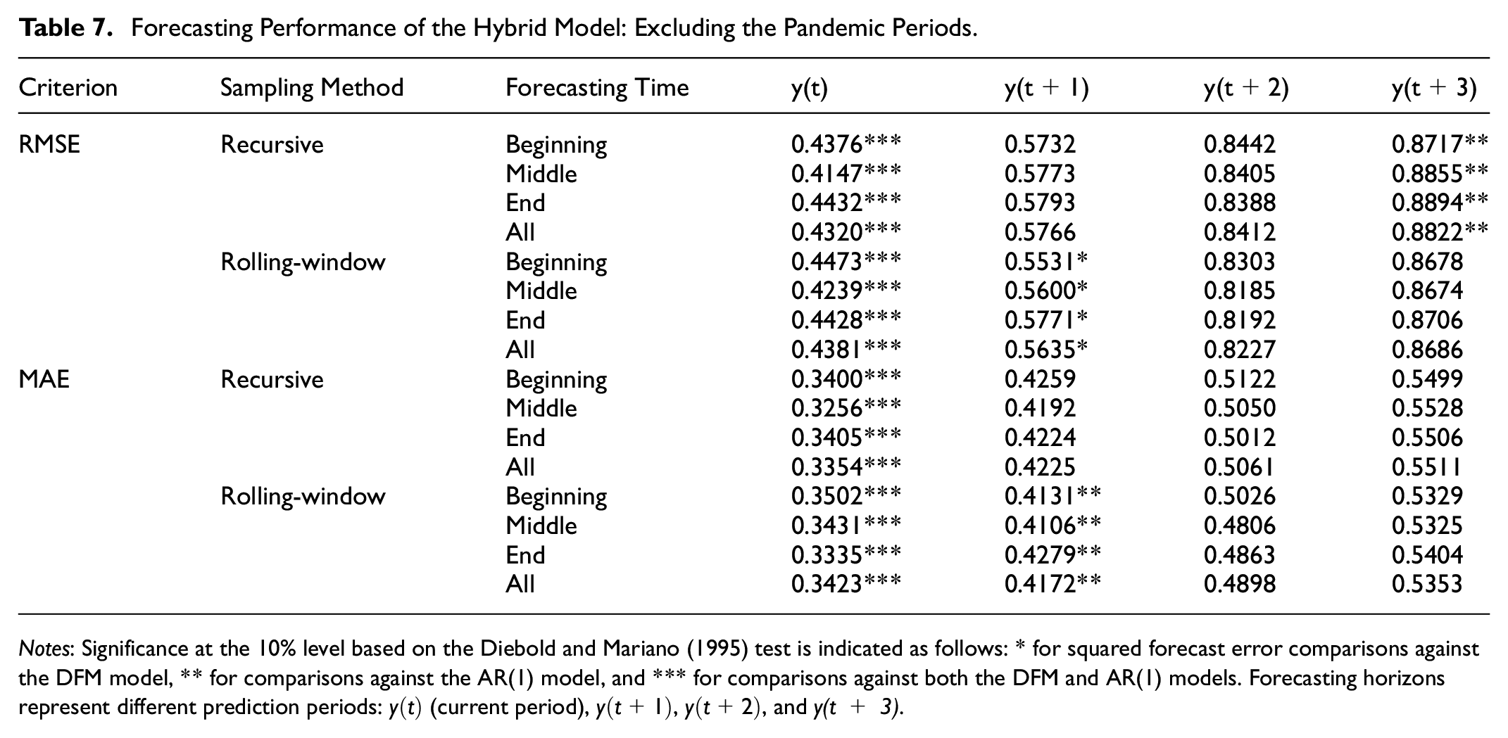
Notes: Significance at the 10% level based on the Diebold and Mariano (1995) test is indicated as follows: * for squared forecast error comparisons against the DFM model, ** for comparisons against the AR(1) model, and *** for comparisons against both the DFM and AR(1) models. Forecasting horizons represent different prediction periods: $y\left(t\right)$ (current period), $y(t+1)$ , $y(t+2)$ , and y(t + 3).

Under rolling-window sampling, the hybrid model maintains strong performance, though its advantage diminishes slightly compared to recursive sampling. This suggests that the model’s design effectively utilizes cumulative historical data, which is especially advantageous in recursive sampling setups. The MAE values further support this trend, showcasing the hybrid model’s consistent ability to minimize forecast deviations, even for the current quarter.

During the periods including the pandemic, forecasting becomes inherently more challenging due to heightened volatility and structural economic changes. However, the hybrid model proves its adaptability, as evidenced by its lower RMSE and MAE compared to standalone models, as shown in Table 8. For instance, under recursive sampling with the pandemic, the hybrid model records an RMSE of 0.7734 for the current quarter forecast ( $y\left(t\right)$ ) at the middle forecasting point, outperforming standalone approaches that struggle with capturing the complexities of pandemic-induced disruptions. This result underscores the hybrid model’s ability to integrate traditional econometric robustness with the nonlinear learning capabilities of LSTM and GRU, ensuring resilience in volatile environments.

Table 8.

Forecasting Performance of the Hybrid Model: Including the Pandemic Periods.

Criterion	Sampling Method	Forecasting Time	y(t)	y(t+1)	y(t+2)	y(t+3)
RMSE	Recursive	Beginning	0.7986***	0.8883	0.8635	0.8515**
		Middle	0.7734***	0.8496	0.8302	0.8379**
		End	0.7367***	0.8448	0.8773	0.8748**
		All	0.7700***	0.8611	0.8572	0.8548**
	Rolling-window	Beginning	0.8303***	0.847*	0.8446	0.8315
		Middle	0.8264***	0.8381*	0.8243	0.8250
		End	0.8751***	0.8514*	0.8448	0.8445
		All	0.8442***	0.8455*	0.8380	0.8337
MAE	Recursive	Beginning	0.5180***	0.5835	0.5620	0.5666
		Middle	0.4926***	0.5513	0.5328	0.5423
		End	0.4928***	0.5632	0.5629	0.5785
		All	0.5011***	0.5660	0.5526	0.5625
	Rolling-window	Beginning	0.5399***	0.5535**	0.5458	0.5263
		Middle	0.5330***	0.5441**	0.5188	0.5180
		End	0.5332***	0.5662**	0.5298	0.5522
		All	0.5354***	0.5546**	0.5314	0.5322

Notes: Significance at the 10% level based on the Diebold and Mariano (1995) test is indicated as follows: * for squared forecast error comparisons against the DFM model, ** for comparisons against the AR(1) model, and *** for comparisons against both the DFM and AR(1) models. Forecasting horizons represent different prediction periods: $y\left(t\right)$ (current period), $y(t+1)$ , $y(t+2)$ , and $y(t+3)$ .

Across longer forecasting horizons, the hybrid model consistently demonstrates its strength by outperforming individual models. This reflects its ability to effectively combine the strengths of traditional methods with the data-adaptive learning power of machine learning. The meta-learner within the hybrid model dynamically adjusts weights for each base model, leveraging their unique strengths depending on the data context. This adaptability is particularly beneficial in managing the trade-offs between short-term and long-term forecast accuracy.

Overall, the hybrid model’s superior performance across forecasting horizons and sampling methods highlights its robustness and flexibility. Its ability to handle both stable and volatile economic periods, as demonstrated during the pandemic, solidifies its value as a reliable and advanced tool for economic forecasting. These findings align with the growing consensus in economic forecasting research, emphasizing the importance of integrating traditional and machine learning-based approaches to achieve greater predictive accuracy in complex and dynamic economic environments.

From a theoretical standpoint, LSTM and hybrid models align closely with economic principles by effectively modeling heterogeneity and capturing structural breaks. In economic systems, the relationships among variables are rarely static; they evolve in response to policy changes, market innovations, and exogenous shocks. LSTM’s adaptive learning framework, enabled by its ability to retain and update information through sequential data processing and memory retention mechanisms, allows it to adjust to such changes without requiring explicit structural modifications, as is often necessary in traditional models. This capability makes LSTM particularly effective in capturing nonlinear dynamics and evolving dependencies in economic data.

Hybrid models further enhance forecasting robustness by leveraging the complementary strengths of traditional econometric and machine learning approaches. Traditional models, such as the Dynamic Factor Model (DFM), provide a strong theoretical foundation and interpretability, excelling at capturing linear relationships and economic theory-driven structures. Machine learning models, on the other hand, bring flexibility and adaptability, allowing them to uncover complex patterns and nonlinear relationships that are often hidden in the data. By dynamically combining forecasts from these models, hybrid approaches offer resilience to regime shifts, structural breaks, and nonstationarity in economic environments. For instance, hybrid models can adjust to changing economic conditions, such as policy interventions or financial crises, by weighting the contributions of each underlying model based on their predictive strengths in specific scenarios.

This integration of traditional and machine learning approaches ensures that hybrid models not only produce accurate and robust forecasts but also maintain relevance across diverse economic conditions. Their ability to handle regime shifts and structural changes, combined with their adaptability to evolving data patterns, positions hybrid models as a practical and theoretically sound solution for modern economic forecasting challenges. With empirical studies consistently demonstrating their superior performance during periods of volatility and uncertainty, these models have emerged as a critical tool for policymakers and researchers navigating increasingly complex macroeconomic landscapes.

Model Robustness and Real-World Applicability

Ensuring robustness and real-world applicability was a central focus of the forecasting models in this study. Robust design measures and dynamic forecasting frameworks were integrated to enhance both reliability and practical utility.

Model robustness was achieved through techniques designed to adapt to evolving economic conditions. Rolling window forecasting retrained the models periodically with the most recent data, ensuring adaptability to structural shifts by prioritizing updated information and reducing the impact of outdated patterns. Recursive forecasting further enhanced adaptability by progressively expanding the training dataset as new outcomes became available, improving learning capacity and ensuring predictions reflected current economic dynamics.

To assess consistency and reliability, the study adopted a multi-horizon forecasting framework. This approach evaluated model performance across different forecasting horizons, from current period predictions to multi-step-ahead forecasts, demonstrating reliability in both short-term and medium-term scenarios. A validation split reserved 25% of the training data for assessing performance on unseen data, ensuring effective generalization and robustness to variations in input features.

The practical utility of these robust models is evident in their applicability to real-world economic decision-making. By combining traditional econometric models like AR(1) and DFM with advanced machine learning architectures such as LSTM and GRU, the study captured both linear and nonlinear dependencies in economic time series. This hybrid framework offers versatility in handling diverse economic conditions, from periods of stability to volatility. The rolling and recursive forecasting methods further enhance the models’ adaptability, allowing them to dynamically update predictions as new data becomes available. This flexibility is particularly valuable for institutions such as central banks and policy agencies, where timely and accurate forecasts are critical for informed decision-making.

While the primary focus of the study is on GDP growth, the proposed methodology is designed to be scalable to other macroeconomic indicators such as inflation rates, unemployment rates, or consumer spending. This scalability enhances the utility of the forecasting framework across a wide range of economic applications. Additionally, the inclusion of interpretable models such as AR(1) and DFM alongside advanced machine learning models as well as the hybrid model ensures transparency in the forecasting process. Policymakers and analysts can rely on the simpler models for intuitive insights while leveraging the predictive power of the advanced models to capture complex patterns. This dual focus on simplicity and sophistication enhances the practical relevance of the framework.

Finally, the use of dynamic forecasting frameworks mirrors real-world economic conditions, where data is subject to continuous updates. By replicating these dynamic scenarios, the study demonstrates the robustness and applicability of the models in practical forecasting environments. The integration of these measures ensures that the proposed framework is not only statistically reliable but also practically relevant.

Discussion and Conclusion

This study explores the integration of traditional econometric models and advanced machine learning techniques, particularly LSTM and GRU algorithms, to forecast South Korea’s GDP amidst a rapidly evolving economic landscape influenced by global crises such as the COVID-19 pandemic and ongoing geopolitical tensions. By leveraging the complementary strengths of these approaches, the study advances the field of economic forecasting, providing robust methodologies that adapt to complex and volatile economic conditions.

A detailed comparison between GRU and LSTM models reveals distinct advantages and situational benefits of each approach. LSTM models are designed to capture long-term dependencies within sequential data by leveraging their memory cell architecture and gating mechanisms. This makes LSTM particularly effective in economic scenarios where long historical trends or cyclical patterns significantly influence future outcomes. For instance, LSTM demonstrated strong performance during periods of structural change and heightened volatility, such as the COVID-19 pandemic. However, this complexity comes at the cost of higher computational demands, making LSTM models less suitable for applications requiring rapid deployment or real-time predictions.

Conversely, GRU models, which employ a simplified gating mechanism, offer computational efficiency while maintaining competitive accuracy for shorter-term forecasts. The reduced complexity of GRU allows for faster training times, making it a viable alternative for scenarios with limited computational resources or when dealing with less complex data patterns. While GRU may underperform LSTM in modeling intricate dependencies, its adaptability and efficiency make it an attractive option for real-world applications requiring rapid insights. By comparing these models, the study highlights their situational advantages, emphasizing the importance of selecting the appropriate model based on the specific economic forecasting context and data characteristics.

The introduction of a hybrid framework further enriches this study by integrating the strengths of both traditional econometric and advanced machine learning models. Traditional econometric models, such as AR and DFM, provide interpretability and theoretical grounding, enabling researchers to identify clear relationships between economic variables. However, these models often struggle to capture nonlinear dependencies and adapt to rapid structural changes. In contrast, machine learning models, such as LSTM and GRU, excel in these areas by leveraging their capacity to learn complex patterns from data. The hybrid framework dynamically combines these strengths using a meta-learner, which assigns optimal weights to the forecasts of individual models.

This meta-learner-based hybrid model not only improves forecasting accuracy but also ensures robustness across diverse economic scenarios. For example, during periods of economic stability, the hybrid model benefits from the precision and interpretability of econometric methods, while during periods of volatility, it relies on the adaptability of machine learning models to capture nonlinear dynamics and unexpected trends. The results demonstrate that the hybrid model consistently outperforms standalone approaches, underscoring its effectiveness in balancing theoretical insights and predictive adaptability.

While the study presents a robust framework, it is important to acknowledge potential limitations and challenges. The reliance on historical data patterns introduces risks when structural changes or unprecedented shocks occur. For instance, models trained on pre-pandemic conditions may struggle to predict post-pandemic outcomes where traditional economic relationships no longer apply.

Another potential limitation lies in the choice of base models. While the inclusion of LSTM, GRU, DFM, and AR(1) offers a blend of traditional and advanced approaches, this selection may exclude other models that could potentially improve performance. The reliance on specific model architectures introduces the possibility of model-specific biases influencing the results. Future work could explore a broader range of models to determine whether the inclusion of additional methods improves forecast accuracy and robustness.

Additionally, the computational demands of advanced machine learning models, particularly LSTM, remain a concern. These demands are amplified during hyperparameter tuning, where extensive trial-and-error processes are required to optimize model performance. GRU, with its more efficient architecture, mitigates some of these challenges but may sacrifice performance in modeling long-term dependencies.

Another computational concern arises from the scalability of the proposed models. As the size and complexity of the input data increase, so does the demand for memory and processing power. This can lead to delays in training and inference, especially when dealing with high-frequency economic data or when forecasting over extended horizons. While simpler architectures like traditional econometric models like AR(1) can mitigate some of these issues, trade-offs between accuracy and computational efficiency often remain.

Future research could enhance the hybrid model by incorporating real-time data updates and nowcasting techniques. By integrating high-frequency data, such as financial market indicators or online search trends, the hybrid framework could become even more responsive to rapidly changing economic conditions. Advanced ensemble learning methods, such as boosting or stacking, could also refine the meta-learner’s weighting mechanism, improving both accuracy and interpretability. Additionally, expanding the application of these models to other macroeconomic variables or regional economies would further test their generalizability and robustness. Techniques like transfer learning or domain adaptation could enable these models to perform well in contexts with limited or noisy data, such as emerging economies.

By addressing these challenges and opportunities, the study underscores the importance of balancing model sophistication with practical considerations, paving the way for broader adoption of advanced and hybrid forecasting techniques in real-world economic applications. The findings highlight the potential of integrating traditional econometric methods with modern machine learning models to enhance the forecasting toolkit, providing actionable insights for researchers, policymakers, and practitioners navigating the complexities of modern economic decision-making.