Sage Journals: Discover world-class research

Abstract

The primary goal of exploratory factor analysis (EFA) is to determine the number of factors and their structure. Thus, the decision on the number of factors to retain is crucial. Nevertheless, researchers frequently overlook the precision of factor retention techniques and opt for unreliable methodologies instead. The objective of this study is to compare the efficiency of utilizing root mean square error of approximation (RMSEA) and parallel analysis (PA) methods for retaining factors in exploratory factor analysis (EFA). Two methods for comparing RMSEA, namely root deterioration per restriction (RDR) and RMSEA difference test, are employed for nested models. Although researchers use RMSEA to compare two different models, no studies have compared RMSEA and RDR methods. Thus, this study examined three different methods for factor retention. Monte-Carlo simulations were utilized to evaluate the accuracy of RDR compared to RMSEA difference testing and PA. The simulations show that RDR performs better than RMSEA difference testing and PA when the number of variables per factor is low. However, as the number of variables per factor increases, PA becomes more effective. This study provides guidance to researchers using EFA to select factor retention methods that suit different conditions.

Plain Language Summary

Study for what methods to use when determining the number of latent variables or factors.

The study was conducted to compare methods for determining the number of factors in exploratory factor analysis (EFA). Researchers conducted a simulation study to assess the performance of these methods under various conditions. The findings of the study indicate that root deterioration per restriction (RDR) outperforms RMSEA difference testing and parallel analysis (PA) when the number of variables per factor is low. However, as the number of variables per factor increases, PA becomes more effective. These findings provide valuable guidance for researchers using EFA, helping them to select appropriate factor retention methods based on the specific conditions of their study. In practical terms, the study suggests that using RDR is recommended, particularly when dealing with small sample sizes and a low number of variables per factor. This recommendation can assist researchers in making informed decisions when conducting factor analysis and interpreting the results accurately.

Keywords

exploratory factor analysis model fit index root mean square error of approximation root deterioration per restriction parallel analysis

Introduction

The creation of psychological scales has been a subject of debate. These scales concentrate on assessing underlying concepts or factors that cannot be evaluated directly, unlike other forms of measurement. Exploratory factor analysis (EFA) has been devised to investigate the hidden structure of psychological and organizational behavioral constructs (Coker et al., 2018), utilizing the correlation between variables to give rise to a factor. Exploratory factor analysis (EFA) is frequently utilized in developing new scales and applying existing scales to provide conclusive evidence for the factors associated with the scale, even when no factors can be specified based on theoretical foundations (Achim, 2020; Widaman, 2018). Therefore, appropriate consideration should be given to this vital aspect of the research process. Determining the optimal number of factors is crucial to ensure that the factor model includes all factors of substantive importance while excluding any spurious ones (Auerswald & Moshagen, 2019; Braeken & van Assen, 2017).

The problem of the issue lies in the often-overlooked precision of factor retention methods within exploratory factor analysis (EFA). Despite its fundamental importance, researchers frequently rely on unreliable methodologies, neglecting the critical decision of how many factors to retain and their structure. Goretzko et al. (2019) examined psychological studies using EFA methods from 2007 to 2017. Among 304 articles, the most frequently used criterion was the Kaiser-Guttman criterion (K1; Eigenvalue > 1), applied in 55.6% of cases, followed by the scree test (46.4%), Parallel Analysis (PA; 42.1%), and theoretical considerations or interpretability of the solution (35.5%). Although most researchers used multiple methods to determine factors, the Kaiser-Guttman rule and scree test were still the most employed. This oversight underscores the need for a thorough investigation into the comparative efficacy of retention techniques, thus prompting this study. By addressing this gap, this study aims to provide clarity and guidance to researchers grappling with factor retention decisions in EFA.

The retention of factors plays a pivotal role in EFA because under-factoring (extracting too few factors) or over-factoring (extracting too many factors) can generate factors that are non-interpretable or unreliable (Garrido et al., 2012). This may result in inaccurate theoretical formulations. The primary objective of this study is to compare the efficacy of three factor retention strategies in EFA: RMSEA difference test, root deterioration per restriction (RDR), and parallel analysis (PA). In past studies, to establish the most suitable number of factors, Clark and Bowles (2018) carried out research using the model fit index (MFI) which includes RMSEA, the comparative fit index (CFI), and the Tucker-Lewis index (TLI) in EFA. They illustrated that the use of MFI can effectively detect under-factored solutions. Additionally, Finch (2020) compared the performance of parallel analysis (PA) with MFI fit differences and discovered that RMSEA difference test was a reliable choice. Savalei et al. (2021) proposed employing root deterioration per restriction (RDR; Browne & Du Toit, 1992) for comparing stability between two nested models. RDR has the advantage of using the same metric and cutoffs as RMSEA. While the efficiency of root mean square error of approximation (RMSEA) in exploratory factor analysis (EFA) has been widely recognized, its suitability within the context of EFA remains unexplored. Therefore, it is imperative to investigate its performance. This research aims to test the efficacy of using RDR and RMSEA in determining the number of factors, providing insights into their accuracy and preferred implementations. The following sections explain how the RDR and RMSEA difference tests determine the number of factors. Then, a Monte Carlo simulation study is reported, comparing these proposed implementations to the most recommended method, PA, for their effectiveness with simulated datasets.

Literature Review

Exploratory Factor Analysis

The primary goal of EFA is to determine the appropriate number of factors to retain for a given set of variables. Equation 1 shows the fundamental equation for EFA, where x denotes a measured variable, F is a common factor, Λ is a factor loading, and μ represents a unique factor.

x = λ_{1} F_{1} + λ_{2} F_{2} + \dots + λ_{k} F_{k} + μ

(1)

According to Fabrigar et al. (1999), researchers should follow five steps when conducting factor analysis: study design, selection of EFA, factor extraction procedures, selection of number of factors, and selection of factor rotation method. The study design should consider the sample size and the variables to be analyzed to determine whether the EFA approach is appropriate for the purpose of the study. The researcher needs to select an extraction method, such as principal axis factoring or maximum likelihood, which are the two most used methods according to Goretzko et al. (2021). Using the results of eigenvalues derived from extraction methods, researchers determine the number of factors through various factor retention methods. The use of factor retention method is the focus of this study. Finally, the researcher should choose a factor rotation to display the factor loadings for each variable.

Factor Retention Methods

The rules for deciding which factors to retain vary (Garrido et al., 2012), and over the past decades, researchers have suggested numerous methods to determine the exact number of factors (Achim, 2017; Braeken & van Assen, 2017; Golino & Epskamp, 2017; Goretzko & Bühner, 2020; Green et al., 2012; Ruscio & Roche, 2012). Gorsuch (2003, p. 148)divided factor retention methods into two criteria: eigenvalue root criteria and residual criteria. Three factor retention methods use eigenvalues: K1 (Kaiser, 1960), scree tests (Cattell, 1966), PA (Horn, 1965) and Next Eigenvalue Sufficiency Test (NEST; Achim, 2017). On the other hand, determining the number of factors using residual correlations has also been used, including chi-square significance, minimum average partial (MAP; Velicer, 1976), MFIs, and Exploratory Graph Analysis (EGA; Golino & Epskamp, 2017; Golino et al., 2020).

K1 is the most popular and well-known retention method. Theoretically, when there are n factors, all roots in a matrix lead to 1.0. With this principle as the underlying concept, researchers use 1 as the threshold for a decision. Scree testing is another commonly used method. Proposed by Cattell (1966), a scree test plots the given eigenvalues in descending order, and researchers decide based on where the plot appears to level off (i.e., the break point). Scree plots can work well when strong factors are present, but they can be subjective and ambiguous, meaning that different results can be derived from the same data, especially when there are either no clear break points or there are two or more dramatically declining breaks. Numerous simulation studies have shown that the K1 rule leads to over-factoring problems (Cattell & Jaspers, 1967; Hubard & Allen, 1987) and that the ambiguity of the scree test can reduce inter-rater reliability (Crawford & Koopman, 1979; Raiche et al., 2013).

Achim (2017) proposed the NEST method, an iterative approach used to test the hypothesis that a specified number of factors (k) is sufficient to fit a dataset. Starting with k = 0, NEST computes a reference model, generates surrogate datasets, and evaluates eigenvalues to identify additional factors. If the tested eigenvalue exceeds the simulated distribution, it suggests more factors and increments k until no further factors are found. Although some simulation studies (Achim, 2017; Brandenburg, 2024; Brandenburg & Papenberg, 2024) demonstrated NEST’s superiority over methods like PA and EGA, the method is relatively new and not yet widely used in practice. Therefore, this study compared RMSEA and RDR with PA, which is one of the most commonly used retention methods, followed by the K1 criterion and the scree test.

Chi-square significance tests are often used to compare two models when one is a subset of the other and can also be used to compare two EFA models when ML is used. However, chi-squared analysis is known to be sensitive to sample size, which means that it does not represent the accuracy of the model well. On the other hand, MAP (Velicer, 1976) was developed for use in principal component analysis. Each component is partitioned from the correlation matrix and a partial correlation matrix is computed. When the common variance has been removed, leaving the unique variance, the MAP will increase, with the last falling point representing the number of common factors. Some research has shown that MAP is helpful (Velicer et al., 2000), while others have claimed that it leads to under-factoring (Gorsuch, 2003, p. 149). The Model Fit Index (MFI) has recently gained popularity in determining factors. MFI has been widely used in CFA models. Clark and Bowles (2018) focused on the application of cut-off values of MFIs, which are CFI, TLI, and RMSEA. In their study, no single fit statistic performed unambiguously well. Finch (2020) found that all three difference tests of MFI were recommended, but among them, the RMSEA difference test performed better. Considering the previous research, among the eigenvalue root criteria, PA and among the residual criteria, RMSEA will be focused.

EGA estimates the number of dimensions and classification of items based on network psychometrics which examines the relationships between items (Golino & Epskamp, 2017). Following estimation, nodes representing items and edges denoting factor loadings are derived. In factor analysis, nodes correspond to items, and edges represent the relationships between these items and factors (Golino & Epskamp, 2017; Golino et al., 2020). In their study, Golino et al. (2020) conducted a comparison of EGA with various techniques for determining the number of dimensions, including parallel analysis, the K1 rule, and MAP analysis. They found that EGA yielded the most accurate results under specific conditions: a sample size of 5,000, a four-dimensional factor structure, and a correlation of .70 between dimensions yet when the correlation was moderated PA still showed similar results as EGA. EGA was not included in this research due to the focus on comparing the efficacy RMSEA difference test, RDR, and PA in EFA. While EGA has shown promise in previous studies, its omission from our research allows for a more focused examination of these specific factor retention methods within the context of EFA.

Parallel analysis

PA was developed by Horn (1965) to overcome the primary limitation of the Kaiser-Guttman criterion (K1), which overestimates the matrix rank due to sampling error. K1 is based on the population correlation matrix and assumes that the sample size is infinite (Glorfeld, 1995). In reality, a finite sample size tends to cause the first eigenvalue to be computed as greater than 1 and subsequent eigenvalues to be computed as less than 1 due to sampling error and least squares bias (Horn, 1965). PA overcomes the effect of sampling error and is thus a sample-based alternative to the population-based K1 criterion (Carraher & Buckley, 1991; Zwick & Velicer, 1986).PA is based on the premise that real data with a valid underlying factor structure should have larger eigenvalues than parallel components derived from random data with the same sample size and number of variables (Green et al., 2018). By generating random data with the same number of observations (n) and variables (v), the correlation matrix for the data sets is used to extract the eigenvalues. By comparing the eigenvalues of the real and generated data, the number of factors is determined by the point where the last real eigenvalue is higher than the generated eigenvalue.

Zwick and Velicer (1986) examined five commonly used methods for determining dimensionality across conditions as defined by the number of uncorrelated factors, sample size, number of variables per factor, loading size, and factorial complexity. They found that PA was the most accurate approach, but its performance was affected by sample size, factor loading, and number of variables. Several other researchers have concluded that PA is the most effective factor retention method (Golino et al., 2020; Green et al., 2016, 2018; Preacher & MacCallum, 2003). However, when the underlying latent traits are highly correlated with each other, PA has difficulty correctly identifying the number of factors to retain (Caron, 2018).

Model Fit Index

As noted above, RMSEA, TLI, CFI are recommended, but only RMSEA is included in this study. RMSEA is less affected by sample size, takes into account model parsimony, and has guidelines for interpretation. In addition, its distribution has a known confidence interval (CI) following a non-central chi-square distribution, which means it is more informative. This index is calculated using equation (2):

RMSEA = \sqrt{\frac{x^{2} - df}{df (N - 1)}}

(2)

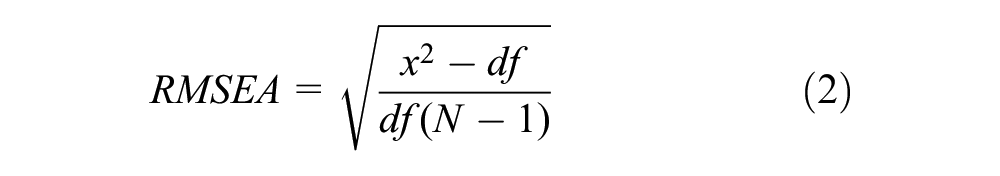
When the RMSEA is 0.05 or less, researchers can conclude that the model has a good fit (Browne & Cudeck, 1993, p. 144). Because RMSEA is a one-tailed test, a value less than 0.05 represents 90% reliability (Hong, 2013, p. 302). After determining the number of factors, it may be helpful to consider the CI. Since RMSEA difference test and RDR are both relative comparisons, when comparing two nested models, it is suggested to consider the absolute value, which is the confidence level, when generalizing the theory.

Determining the Number of Factors to Retain Using RMSEA

The use of MFI to determine the number of factors is not as common in EFA models as it is in CFA models, but simulation studies on the use of MFI have been conducted. Preacher et al. (2013) conducted simulations and reported that the Akaike information criterion (AIC) performed better than the RMSEA. However, recent studies (Barendse et al., 2015; Yang & Xia, 2015) have shown that RMSEA provides accurate results for both continuous and categorical indicator variables. Garrido et al. (2016) compared MFIs with PA and reported that RMSEA produced results comparable in accuracy to those produced by PA. Finch (2020) extended this research and focused on comparing different indices with PA. In this study, MFI outperformed PA for categorical indicators and for normally distributed indicators when factor loadings were small.

There are two ways to compare two nested models using RMSEA: RMSEA difference test (ΔRMSEA) and RDR. Two models are nested, Model A and Model B, where Model B is a more restricted model. In this case, Model B is a subset of the set of all possible covariance matrices implied by Model A, that is, a one-factor model is nested within a two-factor model (Yung et al., 1999).

Since Chen (2007) proposed preliminary cutoffs for ΔRMSEA comparing two nested models based on measurement invariance, chi-squared difference tests have mostly been replaced by MFI differences (Putnick & Bornstein, 2016). ΔRMSEA is calculated as the difference in RMSEA (equation 3):

Δ RMSEA = RMSE A_{B} - RMSE A_{A}

(3)

To determine the number of factors in EFA, Finch (2020) suggested using ΔRMSEA with a cutoff value of 0.015, meaning that if the difference is 0.015 or greater, the fit of the models is different.

Although numerous studies have investigated the use of RMSEA as a factor retention method, they have focused on ΔRMSEA. Meanwhile, RDR (Browne & Du Toit, 1992), which also uses RMSEA to assess model fit, has not been investigated. RDR has the advantage of being a stable population value as sample size increases and is not sensitive to misspecification. Even when the degrees of freedom of model A are large, it provides stable results (Savalei et al., 2021). Despite the suggestions, the performance of ΔRMSEA and RDR methods remains unexplored in the existing literature. Consequently, this study aims to fill this gap by thoroughly investigating the efficacy of RDR within the context of EFA. Therefore, in this study, RDR is investigated (equation 4):

RDR = \sqrt{\frac{F_{0}^{B} - F_{0}^{A}}{d f_{B} - d b_{A}}} = \sqrt{\frac{{(x_{B}^{2} - x_{A}^{2}) - (d f_{B} - d f_{A})}}{(d f_{B} - d f_{A}) (N - 1)}}

(4)

If $(x_{B}^{2} - x_{A}^{2})$ is less than $(d f_{B} - d f_{A})$ , the RDR is set to 0. A RDR of 0.05 or less is used to indicate that the decrease in fit per additional restriction on the model is insignificant.

Study Goals

Recently, PA and MFI have gained considerable interest in research areas for their effectiveness in identifying the optimal number of factors to retain. This study endeavors to pioneer the utilization of RDR in EFA, offering a novel approach to factor retention. The study aims to assess the performance of RDR alongside established methods such as PA and ΔRMSEA, which have been proven effective in previous studies (Finch, 2020; Garrido et al., 2016; Green et al., 2018), across various conditions.

Method

In the present study, simulated data are generated for a common factor model using Monte Carlo simulations. A common factor model is chosen because it includes both major and minor factors, as is commonly the case in real data. Previous studies have generated factor models with simple structures, where each indicator is associated with only one factor and other cross-loadings are set to 0 (Clark & Bowles, 2018; Finch, 2020). In this simulation analysis, however, the presence of minor factors is manipulated. As a result, the simulation results are closer to the real data.

According to Timmerman and Lorenzo-Seva (2011), a common factor model with a limited number of common factors will never fit exactly at the population level, so in simulation analysis it is more reasonable to consider each variable as consisting of a part that is consistent with the common factor model and a part that is not. In this study, data are generated based on equation (5):

Y = ν + Λ η + e

(5)

where Y is an indicator variable with an intercept parameter ν, and Λ is the factor loading matrix, which is interacted with η, an indicator factor, as follows.

In the present study, the manipulated conditions are as follows. The number of factors is set to 3, which is a typical common factor in EFA simulation studies (Clark & Bowles, 2018). The sample size ranges from 100 to 500 with an interval of 100, which is the most common sample size in practice (Goretzko et al., 2021) and like previous studies (Finch, 2020). The number of variables per factor varies from three to eight; three is the minimum required for factor identification (Widaman, 1993), while eight is considered a moderately strong number of variables per factor (Velicer et al., 2000). For factor correlation, moderate (r = .3) and extremely strong (r = .7) correlation levels are included based on Cohen’s (1988) criterion. For each condition, 1,000 data sets are simulated, resulting in a total of 20,000 data sets.

Note that the factor loadings differ within a dataset, that is, the factor loading matrix Λ has different values within a matrix. According to Green et al. (2012), simulation analysis for EFA always uses single factor loadings for all variables. This has been criticized because in empirical data, factor loadings differ from each other.

Therefore, in this study, factor loadings are obtained from real cross-sectional data collected by the Korea National Youth Policy Institute. Specifically, panel data from the 2009 Korean Adolescents’ Game Addiction and Leisure Activity study are used. This basic analysis report was prepared to assess game addiction and family leisure activities among Korean youth by surveying 3,201 middle school students and 3,298 high school students nationwide. Based on the results, measures were developed to promote family leisure activities to prevent game addiction. The data focused on 3,201 middle school students, with 3,065 providing complete responses for this research. Twenty-four items, categorized into three latent satisfaction factors (game addiction, leisure activitiy ability, and leisure activity satisfaction) with eight items each, were used.

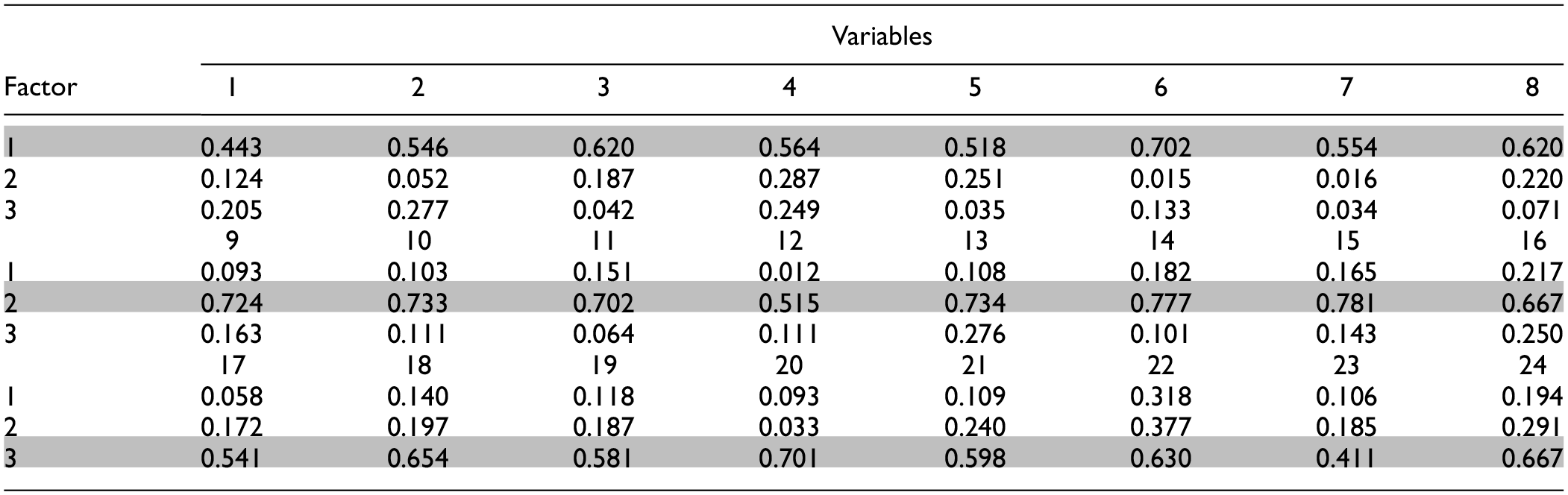
The data is analyzed by Mplus, using Maximum Likelihood (ML) methods for extracting the methods. In this research parallel analysis and RDR is used to determine the number of factors and geomin rotation is used for extracting factor loadings. The factor loadings of the variables are summarized in Table 1. For each replication, the required number of indicators (3 or 8 per factor) are randomly selected from this set of variables.

Table 1.

Variables and Factor Loadings Used in the Present Study.

Methods for Determining the Number of Factors to Retain

This study compares several methods for determining the number of factors to retain. For PA, the 95th percentile (PA95) is used, which is the most recommended PA by several researchers, including Finch (2020). For RMSEA, ΔRMSEA (RMSEA015) and RDR are used. For RMSEA015, the ΔRMSEA cut-off of 0.015 is used to determine the number of factors, as suggested by Chen (2007) and Finch (2020). For RDR, a value of 0.05 or less indicates that the deterioration due to the additional restriction of the model is negligible. A comparison of model fit is made between adjacent factors (e.g., 1 vs. 2, 2 vs. 3, 3 vs. 4). The accuracy of each factor fitting method is evaluated by the proportion of correct estimates. The Monte Carlo simulations and factor analysis for RMSEA and PA are performed using the Mplus program and Mplus automation in R. The Mplus code for data generation and analysis is provided in Appendices 1 and 2.

Results

In this study, 20,000 data sets are generated using Monte Carlo simulations. Each data set is then analyzed with EFA, using MFI and PA to determine the number of factors. The main focus of the study was to determine the proportion of cases in which the correct number of factors was retained using each of the described methods. Additionally, the study recorded the number of factors identified as optimal by each method, along with their convergence rates. It’s important to highlight that if convergence was not achieved for a particular method in each replication, further replications were conducted until 1,000 successful completions were reached.

Minimum Number of Indicators (Three Variables per Factor)

For the lowest number of indicators, each factor is considered to have three variables. The indicators for each factor are randomly selected from Table 1. Figure 1 shows the proportion of cases in which the correct number of factors is identified, which is used as a measure of accuracy when there are three variables for each factor. Regardless of the method used for factor retention, accuracy increases as the sample size increases. In particular, RMSEA015 has an accuracy of 63.6% to 77.1% with a factor correlation of .3 and 61.5% to 73.7% with a factor correlation of .7, and the accuracy increases proportionally to the sample size. However, this accuracy is lower than that of the RDR, which has an accuracy of 91.8% to 98.6% and 92.1% to 98.3% with factor correlations of .3 and .7, respectively, and remains stable with increasing sample size.

Figure 1.

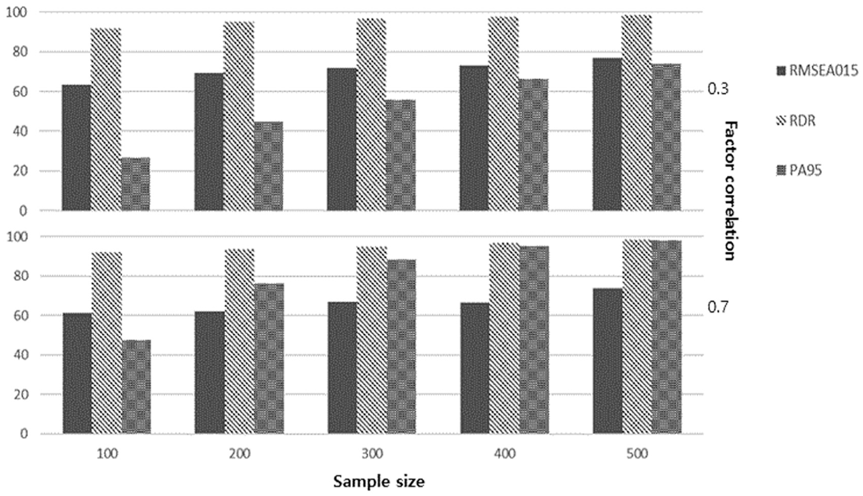
Proportion of correctly identified number of factors according to the factor-retention method, sample size, and factor correlation with three variables per factor.

To focus each factor retention method by sample size and correlation, all other parameters in Table 2 are averaged. PA95 has an accuracy of 26.6% for a sample size of 100, increasing to 74% for a sample size of 500 when the factor correlation is .3, while it has an accuracy of 47.7% to 97.9% when the factor correlation is .7. As shown in Table 2, RDR has high accuracy rates for both tested factor correlations and all five sample sizes. RMSEA015 has higher accuracy for the low factor correlation, while PA95 performs better for the high factor correlation. For a factor correlation of .3, RDR (96.06%) has the highest accuracy, followed by RMSEA015 (71.00%) and PA95 (53.48). When the factor correlation is .7, RDR (95.06%) also has the highest accuracy, followed by PA95 (81.12%) and RMSEA015 (66.18%).

Table 2.

Proportion of Correctly Identified Number of Factors for Each Factor-Retention Method in Accordance with Sample Size or Factor Correlation with Three Variables per Factor.

Parameters	RMSEA₀₁₅	RDR	PA₉₅
Correlation
.3	71.00	96.06	53.48
.7	66.18	95.06	81.12
Sample size
100	62.55	91.95	37.15
200	65.75	94.40	60.60
300	69.50	95.80	72.10
400	69.75	97.20	80.70
500	75.40	98.45	85.95

With a sample size of 100, RDR is the most accurate factor retention method with an accuracy of 91.95%, followed by RMSEA015 (62.55%) and PA95 (37.15%). When the size is 300, the order changes slightly: RDR (95.80%), PA95 (72.1%), and RMSEA015 (69.5%). When the sample size is 500, the accuracy for RDR, PA95, and RMSEA015 are 98.45%, 85.95%, and 75.40%, respectively.

Moderately Strong Number of Indicators (eight Variables per Factor)

Figure 2 shows the proportion of cases in which the correct number of factors is retained by method, sample size, and factor correlation when the factors have eight indicators. As the sample size increases, all methods become more accurate. Note that PA95 has high accuracy regardless of factor correlation and sample size.

Figure 2.

Proportion of correctly identified number of factors according to the factor-retention method, sample size, and factor correlation with eight variables per factor.

For RMSEA₀₁₅, the accuracy rate increases with increasing sample size from 56.4% to 97.9% for a factor correlation of .3, and from 72.4% to 98.6% for a factor correlation of .7. With a factor correlation of .3, RDR has an accuracy of 67.8% for a sample size of 100, increasing to 79.5% for a sample size of 300, and to 92.9% and 98.3% for sample sizes of 400 and 500, respectively. When the factor correlation is .7, the accuracy is 37.9% for a sample size of 100, increasing to 97.8% for a sample size of 500. PA₉₅ also shows accuracy rates of 73.6% and 98.8% for a sample size of 100 for factor correlations of .3 and .7, rising to 100% for the other conditions.

Table 3 shows the accuracy of the factor retention methods for the two factor correlations. When the factor correlation is low (.3) the accuracy rates are 94.72% for PA₉₅, 84.92% for RMSEA₀₁₅, and 82.48% for RDR. When the factor correlation is high (.7), the accuracy rates are 99.76%, 88.94%, and 76.48% for PA₉₅, RMSEA₀₁₅, and RDR, respectively.

Table 3.

Proportion of Correctly Identified Number of Factors for Each Factor-Retention Method in Accordance with Sample Size or Factor Correlation with Eight Variables per Factor.

Parameters	RMSEA₀₁₅	RDR	PA₉₅
Correlation
.3	84.92	82.48	94.72
.7	88.94	76.48	99.76
Sample size
100	64.40	52.85	86.20
200	82.90	74.85	100.00
300	93.05	78.90	100.00
400	96.05	92.75	100.00
500	98.25	98.05	100.00

When considering sample size, PA₉₅ performs well with an accuracy rate of 100% when the sample size is 200 or greater. For RMSEA₀₁₅ and RDR, starting from 64.4% and 52.85%, the accuracy rate increases to 98.25% and 98.05% when the sample size is 500.

Under-factoring and Over-factoring Issues

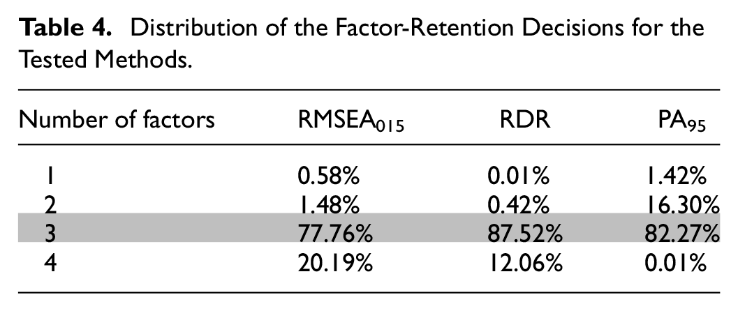
Table 4 summarizes the number of factors retained by each of the tested factor retention methods. RDR produces the most accurate results with an accuracy rate of 87.52%, followed by RMSEA₀₁₅, and RDR produces more over-factoring results, with 20.19% and 12.06% of cases identifying four factors, respectively, while PA₉₅ has under-factoring problems, with a higher percentage of cases identifying one or two factors than four factors.

Table 4.

Distribution of the Factor-Retention Decisions for the Tested Methods.

Discussion

With the increasing use of EFA for various purposes, such as confirming the parceling of SEM (Asparaouhov & Muthen, 2009), determining the number of factors to retain in EFA has been crucial. Many researchers continue to use methods that have been shown to perform poorly (Goretzko et al., 2021; Henson & Roberts, 2006; Kang et al., 2013). For example, Goretzko et al. (2021) found that 55.6% of articles used the K1 criterion and 46.4% used scree tests, despite previous simulation studies concluding that PA performs better (Fabrigar et al., 1999). Interestingly, those who cited Fabrigar’s study showed different results, with 88% using PA. However, K1 and scree tests were still reported together, indicating that there is still a demand for retention methods to replace K1 and scree tests.

This study aimed to provide a comprehensive comparison of the performance of RDR, RMSEA, and PA. Despite the acknowledged accuracy of these methods, no prior research has directly compared all three, with some studies solely focusing on RMSEA (Finch, 2020). Previous investigations predominantly centered on the use of MFIs with specified cutoff points or for difference tests of MFIs (Clark & Bowles, 2018; Finch, 2020). The widespread popularity of RMSEA comparisons is evident, as evidenced by the substantial citation count of Chen (2007). Notably, RDR, initially proposed by Browne and Du Toit (1992), has garnered attention for its utilization in comparing nested models using the RMSEA index (Savalei et al., 2021). This study uniquely focuses on comparing RMSEA with RDR and PA, contributing to the existing literature by elucidating their relative efficacy.

The results show that, in general, all methods have a higher accuracy rate as the sample size increases. When the factor correlation is low, RDR is the best performing option, while PA is more accurate when the factor correlation is high. In fact, the accuracy of PA has been demonstrated in various studies (Golino et al., 2020; Green et al., 2018; Velicer et al., 2000), and it has also been shown that the accuracy of PA increases as the sample size increases (Crawford et al., 2010; Finch, 2020).

Simulation results indicate that using MFIs as a factor retention method has advantages under certain conditions, especially when the number of variables per factor is small, and the factor correlation is low (Finch, 2020). Finch reported that when the sample size is small, RMSEA015 has a low accuracy rate, although it outperforms CFI and PA. In this study, when the number of variables per factor is low, RDR has the highest accuracy rate of more than 90%, regardless of sample size. As the number of variables per factor increases, the accuracy of RDR and RMSEA becomes lower than PA. However, with increasing sample size, more accurate results are expected regardless of the method used. RMSEA and RDR are more likely to over-factor, while PA is more susceptible to under-factoring. Monte Carlo simulation studies are valuable for illustrating the effects of methods in different situations but are criticized for using artificial data. To address this, the study generated data reflecting real values.

Since no unanimously accepted method exists, using multiple methods to check for consensus is recommended. Over half of recent research reports more than one factor retention criterion (Goretzko et al., 2021), typically K1 and scree test, followed by PA, with theory and interpretability as the fourth common method. Note that except PA, K1 and scree test are not recommended due to their ambiguity. Agreement among methods is not guaranteed but is likely accurate when present (Ruscio et al., 2010). Thus, choosing an accurate method is crucial when conducting EFA.

This study finds that RDR has a high overall accuracy rate across all conditions (87.52%). In particular, it outperforms all other factor retention methods when the number of variables is low. However, as the number of variables increases (eight per factor), it has a lower accuracy rate than other methods, although an increase in sample size improves its accuracy. Interestingly, PA, which is known to be an effective tool for EFA, has a lower accuracy rate than RDR when the number of variables per factor is low. In addition, RMSEA, which has been highlighted for its accuracy in determining the number of factors in EFA, also has a lower accuracy rate when the number of variables per factor is three, and a similar accuracy rate with eight variables per factor compared to RDR. Thus, while PA can be an effective method, RDR may be the best choice for researchers when the number of variables per factor is small.

The problem of under-factoring and over-factoring still exists. RDR and RMSEA are effective in avoiding under-factoring, which is consistent with Clark and Bowles (2018), who reported that MFIs perform well in terms of preventing under-factoring. However, over-factoring is a problem for the MFIs in the present study. In contrast, inaccuracies in the use of PA are mostly due to under-factoring. Thus, the use of both RMSEA and PA can compensate for under-factoring and over-factoring problems.

This study has several limitations. Firstly, it did not consider factors such as data characteristics, response categories, and skewness. Previous research has demonstrated the effectiveness of MFIs in complex EFA models and with categorical data, suggesting the need for more nuanced models in further analysis (Clark & Bowles, 2018). Additionally, the study solely focused on one MFI, RMSEA, while other indices such as the CFI and TLI have suggested cutoffs and difference tests for factor retention. Although Finch (2020) found CFI and TLI to be less accurate than RMSEA, exploring alternative cutoffs with more intricate data could yield valuable insights. Furthermore, the growing utilization of EGA and machine learning in EFA presents promising avenues for future research. Moreover, NEST method suggested by Achim (2017) also can be compared as well. Comparing RMSEA and RDR with EGA and NEST, particularly in scenarios with high factor correlations, could offer intriguing comparative insights into their respective accuracies.

The study makes several significant contributions to the field of EFA. It offers a comprehensive comparison of three prominent factor retention methods: RMSEA, RDR, and PA. By evaluating their performance under various conditions, the study provides valuable insights into the relative efficacy of these methods in determining the optimal number of factors to retain. Furthermore, the study addresses the gap in the existing literature by directly comparing RMSEA, RDR, and PA, which have not been thoroughly investigated together before. This contributes to a more thorough understanding of the strengths and limitations of each method, allowing researchers to make informed decisions when conducting EFA. Moreover, when researchers choose PA and RMSEA or RDR for their research, they are analyzing one method from eigenvalue root criteria and the other from residual criteria. This approach allows their research to cover both factor retention areas. Since RMSEA and RDR are derived from the RMSEA index of structural equation modeling, which most researchers are familiar with nowadays, the analysis process is much easier than with other factor retention methods.

In conclusion, using MFIs in EFA can be an effective solution in determining the number of factors. The present study suggests that using RDR may be the best choice, especially when the sample size and the number of variables per factor are small. After deciding the number of factors by RDR, the researcher can consider the CI of RMSEA. CI can help the researcher to generalize the research. In addition, PA and RMSEA can compensate each other, so it is recommended to use these retention methods together.

Footnotes

Appendix 1

Appendix 2 Declaration of Conflicting Interests

The author(s) declared no potential conflicts of interest with respect to the research, authorship, and/or publication of this article.

Funding

The author(s) received no financial support for the research, authorship, and/or publication of this article.

ORCID iDs

Sangyoug Bae

Sehee Hong

Data Availability Statement

The data supporting the findings of this study were generated using the methodology outlined in the appendix. The appendix provides detailed instructions and necessary resources for replicating the data generation process.

Lee K. Survey on Adolescents’ Game Addiction and Leisure Activities, 2009 [Data set]. National Youth Policy Institute [Research Institute]. Korea Social Science Data Archive (KOSSDA) [Data Provider], 2010-08-25, .

References

Achim

(2017). Testing the number of required dimensions in exploratory factor analysis. The Quantitative Methods for Psychology, 13(1), 64–74. https://doi.org/10.20982/tqmp.13.1.p064

Achim

(2020). Esprit et enjeux de l’analyse factorielle exploratoire. [Spirit and issues of exploratory factor analysis.]. The Quantitative Methods for Psychology, 16(4), 213–247. https://doi.org/10.20982/tqmp.16.4.p213

Asparaouhov

Muthen

(2009). Exploratory structural equation modeling. Structural Equation Modeling: A Multidisciplinary Journal, 16(3), 397–438.

Auerswald

Moshagen

(2019). How to determine the number of factors to retain in exploratory factor analysis: A comparison of extraction methods under realistic conditions. Psychological Methods, 24(4), 468–491. https://doi.org/10.1037/met0000200

Barendse

M. T.

Oort

F. J.

Timmerman

M. E.

(2015). Using exploratory factor analysis to determine the dimensionality of discrete responses. Structural Equation Modeling, 22(1), 87–101.

Braeken

van Assen

M. A.

(2017). An empirical Kaiser criterion. Psychological Methods, 22(3), 450–466. https://doi.org/10.1037/met0000074

Brandenburg

(2024). Factor retention in ordered categorical variables: Benefits and costs of polychoric correlations in eigenvalue-based testing. Behavior Research Methods, 56, 7241–7260. https://doi.org/10.3758/s13428-024-02417-0

Brandenburg

Papenberg

(2024). Reassessment of innovative methods to determine the number of factors: A simulation-based comparison of exploratory graph analysis and Next Eigenvalue Sufciency Test. Psychological Methods, 29(1), 21–47.

Browne

M. W.

Cudeck

(1993). Alternative ways of assessing model fit. In Bollen

K. A.

Long

J. S.

(Eds.), Testing structural equation models (pp. 136–162). Sage.

10.

Browne

M. W.

Du Toit

S. H.

(1992). Automated fitting of nonstandard models. Multivariate Behavioral Research, 27(2), 269–300. https://doi.org/10.1207/s15327906mbr2702_13

11.

Caron

P.-O.

(2018). Minimum average partial correlation and parallel analysis: The influence of oblique structures. Communications in Statistics–Simulation and Computation, 48(7), 2110–2117.

12.

Carraher

S. M.

Buckley

M. R.

(1991). The effect of retention rule on the number of components retained: The case of the pay satisfaction questionnaire. In Proceedings of the Southern management association (pp. 247–249).

13.

Cattell

R. B.

(1966) The scree test for the number of factors. Multivariate Behavioral Research, 1, 245–276.

14.

Cattell

R. B.

Jaspers

(1967). A general plasmode (No. 30-10-5-2) for factor analytic exercises and research. Multivariate Behavioral Research Monographs, 67(3), 211.

15.

Chen

F. F.

(2007). Sensitivity of goodness of fit indexes to lack of measurement invariance. Structural Equation Modeling, 14, 464–504.

16.

Clark

D. A.

Bowles

R. P.

(2018). Model fit and item factor analysis: Overfactoring, underfactoring, and a program to guide interpretation. Multivariate Behavioral Research, 53, 544–558.

17.

Cohen

(1988). Statistical power analysis for the behavioral sciences (2nd ed.). Erlbaum.

18.

Coker

J. L.

Catlin

Ray-Griffith

Knight

Stowe

Z. N.

(2018). Buprenophrine medication-assisted treatment during pregnancy: An exploratory factor analysis associated with adherence. Drug and Alcohol Dependence, 192, 146–149.

19.

Crawford

Green

S. B.

Levy

W. J.

Scott

Svetina

D. S.

Thompson

M. S.

(2010). Evaluation of parallel analysis methods for determining the number of factors. Educational and Psychological Measurement, 70, 885–901.

20.

Crawford

Koopman

(1979). Note: Inter-rater reliability of scree test and mean square ratio test of number of factors. Perceptual and Motor Skills, 49, 223–226.

21.

Fabrigar

L. R.

Wegner

D. T.

MacCallum

R. C.

Strahan

E. J.

(1999). Evaluating the use of exploratory factor analysis in psychological research. Psychological Methods, 4, 272–299.

22.

Finch

W. H.

(2020). Using fit statistic differences to determine the optimal number of factors to retain in an exploratory factor analysis. Educational and Psychological Measurement, 80(2), 217–241.

23.

Garrido

L. E.

Abad

F. J.

Ponsoda

(2012). A new look at Horn’s parallel analysis with ordinal variables. Psychological Methods, 18(4), 454–474.

24.

Garrido

L. E.

Abad

F. J.

Ponsoda

(2016). Are fit indices really fit to estimate the number of factors with categorical variables? Some cautionary findings via Monte Carlo simulation. Psychological Methods, 21, 93–111.

25.

Glorfeld

L. W.

(1995). An improvement on Horn’s parallel analysis methodology for selecting the correct number of factors to retain. Educational and Psychological Measurement, 55(3), 377–393.

26.

Golino

H. F.

Epskamp

(2017). Exploratory graph analysis: A new approach for estimating the number of dimensions in psychological research. PLOS ONE, 12(6), Article e0174035. https://doi.org/10.1371/journal.pone.0174035

27.

Golino

H. F.

Shi

Christensen

A. P.

Garrido

L. E.

Nieto

M. D.

Sadana

Thiyagarajan

J. A.

Martinez-Molina

(2020). Investigating the performance of exploratory graph analysis and traditional techniques to identify the number of latent factors: A simulation and tutorial. Psychological Methods, 25(3), 292–320. https://doi.org/10.1037/met0000255

28.

Goretzko

Bühner

(2020). One model to rule them all? Using machine learning algorithms to determine the number of factors in exploratory factor analysis. Psychological Methods, 25(6), 776–786. https://doi.org/10.1037/met0000262

29.

Goretzko

Pham

T. T. H.

Bühner

(2019). Exploratory factor analysis: Current use, methodological developments and recommendations for good practice. Current Psychology, 40, 3510–3521. https://doi.org/10.1007/s12144-019-00300-2

30.

Goretzko

Pham

T. T. H.

Bühner

(2021). Exploratory factor analysis: Current use, methodological developments and recommendations for good practice. Current Psychology, 40, 3510–3521. https://doi.org/10.1007/s12144-019-00300-2

31.

Gorsuch

R. L.

(2003). Factor analysis. In Weiner

I. B.

Schinka

J. A.

Velicer

W. F.

(Eds.), Handbook of psychology (1st ed., pp. 143–164). John Wily & Sons, Inc.

32.

Green

S. B.

Levy

Thompson

M. S.

(2012). A proposed solution to the problem with using completely random data to assess the number of factors with parallel analysis. Educational and Psychological Measurement, 72(3), 357–374.

33.

Green

S. B.

Redell

Thompson

M. S.

Levy

(2016). Accuracy of revised and traditional parallel analyses for assessing dimensionality with binary data. Educational and Psychological Measurement, 76(1), 5–21.

34.

Green

S. B.

Thompson

M. S.

(2018). Relative accuracy of two modified parallel analysis methods that use the proper reference distribution. Educational and Psychological Measurement, 78(4), 589–604.

35.

Henson

R. K.

Roberts

J. K.

(2006). Use of exploratory factor analysis in published research: Common errors and some comment on improved practice. Educational and Psychological Measurement, 66, 393–416.

36.

Hong

(2013). Basic theory and application of structural equation modeling (p. 302). S&M Research group.

37.

Horn

J. L.

(1965). A rationale and test for the number of factors in factor analysis. Psychometrika, 20, 179–185.

38.

Hubard

Allen

(1987). An empirical comparison of alternative methods for principal component extraction. Journal of Business Research, 15(2), 173–190.

39.

Kaiser

H. F.

(1960). The application of electronic computers to factor analysis. Educational and Psychological Measurement, 20, 141–151.

40.

Kang

Cho.

(2013). A study on the use-realities of exploratory factor analysis in educational research. Educational Measurement Research, 25(3), 521–541.

41.

Preacher

K. J.

MacCallum

R. C.

(2003). Repairing Tom Swift’s electric factor analysis machine. Understanding Statistics, 2, 13–43.

42.

Preacher

K. J.

Zhang

Kim

Mels

(2013). Choosing the optimal number of factors in exploratory factor analysis: A model selection perspective. Multivariate Behavioral Research, 48, 28–56.

43.

Putnick

D. L.

Bornstein

M. H.

(2016). Measurement invariance conventions and reporting: The state of the art and future directions for psychological research. Developmental Review: DR, 41, 71–90. https://doi.org/10.1016/j.dr.2016.06.004

44.

Raiche

Walls

T. A.

Magis

Riopel

Blais

J.-G.

, (2013). Non-graphical solutions for cattell’s scree test. Methodology, 9(1). https://doi.org/10.1027/1614-2241/a000051

45.

Ruscio

Roche

, (2012). Determining the number of factors to retain in an exploratory factor analysis using comparison data of known factorial structure. Psychological Assessment, 24(2), 282–292.

46.

Ruscio

Walters

G. D.

Marcus

D. K.

Kaczetow

(2010). Comparing the relative fit of categorical and dimensional latent variable models using consistency tests. Psychological Assessment, 22, 5–21.

47.

Savalei

Brace

Fouladi

R. T.

(2021, May 9). We need to change how we compute RMSEA for nested model comparisons in structural equation modeling. https://doi.org/10.31234/osf.io/wprg8

48.

Timmerman

M. E.

Lorenzo-Seva

(2011). Dimensionality assessment of ordered polytomous items with parallel analysis. Psychological Methods, 16(2), 209–220.

49.

Velicer

W. F.

(1976). Determining the number of components from the matrix or partial correlations. Psychometrika, 41, 321–327.

50.

Velicer

W. F.

Eaton

C. A.

Fava

J. L.

(2000). Construct explication through factor or component analysis: A review and evaluation of alternative procedures for determining the number of factors or components. In Goffin

R. D.

Helmes

(Eds.), Problems and solutions in human assessment (pp. 41–71). Springer. https://doi.org/10.1007/978-1-4615-4397-8_3

51.

Widaman

K. F.

(1993). Common factor analysis versus principal component analysis: Differential bias in representing model parameter? Multivariate Behavioral Research, 28, 263–311.

52.

Widaman

K. F.

(2018). On common factor and principal component representations of data: Implications for theory and for confirmatory replications. Structural Equation Modeling, 25(6), 829–847. https://doi.org/10.1080/10705511.2018.1478730

53.

Yang

Xia

(2015). On the number of factors to retain in exploratory factor analysis for ordered categorical data. Behavioral Research Methods, 47, 756–772.

54.

Yung

Y. F.

Thissen

McLeod

L. D.

(1999). On the relationship between the higher-order factor model and the hierarchical factor model. Psychometrika, 64, 113–128. https://doi.org/10.1007/BF0229453

55.

Zwick

W. R.

Velicer

W. F.

(1986). Factors influencing five rules for determining the number of components to retain. Psychological Bulletin, 99, 432–442.

Comparison of Factor Retention Methods in Exploratory Factor Analysis: RMSEA,Root Deterioration per Restriction and Parallel Analysis

Abstract

Plain Language Summary

Keywords

Introduction

Literature Review

Exploratory Factor Analysis

Factor Retention Methods

Parallel analysis

Model Fit Index

Determining the Number of Factors to Retain Using RMSEA

Study Goals

Method

Methods for Determining the Number of Factors to Retain

Results

Minimum Number of Indicators (Three Variables per Factor)

Moderately Strong Number of Indicators (eight Variables per Factor)

Under-factoring and Over-factoring Issues

Discussion

Footnotes

Appendix 1

Appendix 2

Declaration of Conflicting Interests

Funding

ORCID iDs

Data Availability Statement

References