Sage Journals: Discover world-class research

Abstract

The aim of the study is the development of methodology for accurate estimation of electric vehicle demand; which is paramount regarding various aspects of the firms decision-making such as optimal price, production level, and corresponding amounts of capital and labor; as well as supply chain, inventory control, capital financing, and operational expenses management. The forecasting methods utilized include statistical techniques (autoregressive integrated moving average [ARIMA], and polynomial regression), machine learning (nonlinear autoregressive neural network [NAR]), deep learning (long short-term memory [LSTM]), hybrid and combination forecasting. With regard to the latter method, our study experiments with four different combining model approaches, including the introduction of an original, novel combining method with the employment of a transcendental LASSO function, which is used to form combinations of forecasts generated by the NAR, ARIMA, and polynomial regression models. The LASSO-based combining model proved superior to all other models, for the majority of forecast error statistics; where the root mean square error (RMSE) and mean absolute percentage error (MAPE) values are 4.5% and 8% respectively lower than the average level of the component model forecasts. The major implications of our empirical findings are that greater accuracy in demand forecasting can be achieved with a combining model approach, rather than reliance on any particular, singular model. Furthermore, given its superior performance, the employment of the studys LASSO-based combining model to forecast electric vehicle demand may lead to optimal firm decision-making over a range of organizational facets, which is predicated on accurate demand function estimation.

Keywords

artificial neural network autoregressive integrated moving average combination forecasting generalized reduced gradient hybrid forecasting least absolute shrinkage and selection operator long short-term memory nonlinear autoregressive neural network polynomial regression weighted least squares

Introduction

The aim of this study is the development of a methodology for accurate estimation of electric vehicle (EV) demand, which is paramount for various aspects of an EV-producing firms decision-making. Specifically, the information contained or reflected in the demand function, such as the amount of planned purchases by consumers over a given price range, and the corresponding price elasticity of demand, helps the firm decide on the optimal production level and the corresponding amount of capital and labor to employ; as well as the product price (Roanec et al., 2021). Additionally, demand forecasting supports almost all business functions, including sales and supply chain management (Chiang et al., 2016; Dolgui & Pashkevich, 2009; Hsieh et al., 2020; Reiner & Fichtinger, 2009); inventory management (Fattah et al., 2018; Nahmias & Tava, 2015), production planning, new capital financing, and operational expenses management cite (Lu et al., 2010; Roanec et al., 2021).

To help facilitate accurate EV demand forecasting with the application of econometrics, both statistical (M. Wang et al., 2015) and machine-learning techniques (Gutierrez et al., 2008; Kochak & Sharma, 2015; Lu et al., 2010) are employed for time-series and multivariate demand forecasting purposes (Roanec et al., 2021). In the process of our analysis, we present a comparative performance of selected multivariate statistical, machine learning (Bishop, 2006; James et al., 2021; Murphy, 2022), and deep learning (Charniak, 2019; Goodfellow et al. 2016) techniques for demand forecasting (F. K. Wang et al., 2011). Univariate damped trend, ARIMA, and polynomial regression models represent classical statistical techniques. NAR and ANN with multi-layer perceptron (MLP) models are selected for machine-learning techniques. LSTM is employed as a deep learning model. Fattah et al. (2018) find that time-series approaches and ANN techniques are two principal approaches much utilized in demand forecasting. With time series modeling, such as moving average, exponential smoothing, and ARIMA, demand forecasts are linear functions of historical data. The ANN, NAR, and LSTM approaches are especially useful with nonlinearity in the data set (Charniak, 2019; James et al., 2021).

We address a research gap in EV demand forecasting by experimenting with a third approach, with models that combine the forecasts generated by both the statistical (ARIMA and polynomial regression) and machine learning (NAR) techniques (Aburto & Weber, 2007; Kim et al., 2021; Mitrea et al., 2009; Y. Wang et al., 2019; G. P. Zhang, 2003). In this way, we incorporate independent information contained in the component models forecasts into the combination forecast in order to achieve greater forecast accuracy (Bates & Granger, 1969; Fair & Shiller, 1990; Terregrossa & Sener, 2023). The specific conceptual idea here is that by forming a combination of forecasts generated separately by an ARIMA model, a polynomial regression model, and a NAR model, we are able to incorporate information regarding both linear and nonlinear functional relations existent in the time-series data set (Kim et al., 2021; Y. Wang et al., 2019; G. P. Zhang, 2003). We form combination forecasts with four different methods: (a) A conventional regression-based method (WLS) (Terregrossa & Ibadi, 2021; Wu & Blake, 2023); (b) The relatively novel gradient algorithm approach (GRG) (Terregrossa & Sener, 2023); (c) An established hybrid model (Kim et al., 2021; Y. Wang et al., 2019; G. P. Zhang, 2003) and the reverse version of that model; (d) Our study also introduces an original, different combining model approach with the employment of the LASSO function to form combinations of forecasts generated by nonlinear autoregressive neural network (NAR), autoregressive moving average (ARIMA), and polynomial regression models which are included to the combining model with an nth order polynomials including square root terms.

With regard to the above-mentioned combining model methods 1, 2, and 4, the conceptual idea is that the output (forecasts) of the component models are used as inputs in the combining model function to generate a combined forecast. However, in hybrid combining models (method 3) the output of a component model is used as input in another component model, to ultimately generate a combination forecast (Terregrossa & Sener, 2023; Y. Wang et al., 2019). Each of these different combining model approaches is referenced and further explained in the subsequent literature review and methodology sections.

With regard to recent methods and ongoing trends in EV research (Haghani et al., 2023) gleaned information from 34,000 articles indexed by the Web of Science (WoS) Core Collection from 1990 to 2021 that have mentioned electric vehicle (EV) in their title or keyword list. In so doing, they have managed to identify distinct trending topics in recent years, by partitioning the time frame from 2016 to 2021 into four approximately equal periods and determining top keywords for each of these periods. They point out that during the first three periods, hybrid EV is the most dominant keyword; however, in the most recent period optimization takes over the top spot (with optimization referring to improved efficiency of EV technology); followed by charging station, wireless power transfer, and EV charging. As noted by Haghani et al. (2023), the development of advanced battery technology, and the resultant emergence of plug-in hybrid EVs and battery-powered EVs, has led to a shift in research efforts toward improved EV technology. And the emergence of the keywords EV-charging and charging station indicates an increased research trend toward EV infrastructure development. Broadbent et al. (2022) have also found charging-infrastructure to be an upward trend in EV research. With the use of a clustering classification, Haghani et al. (2023) have also identified EV-adoption and market development as growing research trends. And they note that increased EV-adoption will lead to increased demand for electricity, which Taalbi and Nielsen (2021) indicate is providing momentum toward the development of cleaner, renewable energy sources to generate electricity. With regard to global EV-market development, the main driving force appears to be government subsidies aimed at R&D and increased production, motivated by environmental concerns such as air quality and resultant political pressure (Altenburg et al., 2022; Iwan et al., 2021).

With regard to the current study, our analysis touches upon the concept of market development, in that our data set of monthly data from 2018 January to 2022 August, which is the EV demand series of Turkey, starts with a few hundred observations and ends with a few thousand; thus tracking the development of the Turkish EV-market from its initial stage to the current period. Our empirical results are thus reflective of the evolving market forces generating EV demand in Turkey, which certainly include environmental as well as economic concerns, leading to political pressure and government involvement. For example, the Turkish government has provided subsidy support to a consortium of domestic firms (TOGG) for the development and production of a Turkish-made EV (also called the TOGG), a brand with national intellectual and industrial property rights; with the explicitly stated aim of contributing to a cleaner air environment by reducing harmful emissions. There is also an optimizing aspect in that TOGG has touted the development of a smart device with a mobility ecosystem encompassing high-end technologies.

Our analysis also includes another type of optimizing aspect, but from a perspective different from the one mentioned above: In the weighted average combination forecast section of our analysis, optimization refers to a process in which the component model forecast weights are determined such that selected forecast error statistics (such as sum of squared error) are minimized (Terregrossa & Sener, 2023; Wu & Blake, 2023). There is also an optimization aspect with regard to our new approach to forming a combining model with the employment of a transcendental LASSO function, which includes a third-order polynomial and a square root term for three-component model forecasts. The transcendental combination function will obviously overfit the forecast because of the excessive number of terms; thus the LASSO operator is used with cross-validation to optimize the combination process by assigning nonzero coefficients to only contributing terms. Cross-validation is useful when the data set is small, which makes it suitable for our case (James et al., 2021; Murphy, 2022). These optimization aspects of the respective combination forecasting methods of the present study are thoroughly explained below, in the subsequent literature review and methodology section.

Literature

In this section, we provide background and context with regard to the development of the forecasting models that are employed in the present study. We begin this treatment with an explanation of a statistical method that has been employed in previous studies to estimate product demand: The autoregressive moving average (ARMA) process, which includes both autoregressive functions (AR) and a finite moving average (MA) process to the forecasting function, which results in more precision and flexibility. Chen et al. (2010) provide an insightful review of the three classes of ARMA models: Moving Average (MA) (q), Autoregressive (AR) (p), and ARMA (p, q); where p is the order of autoregressive, q is the order of moving average; with each class having its own characteristics and suitability for certain situations. They point out that ARMA modeling provides high precision for short-term forecasting, and can be used to reveal the characteristics and dynamic behavior of a time-series. The underlying characteristics of the time-series determine the appropriate model and can be revealed with an evaluation of the autocorrelation and partial autocorrelation functions, which is a process proposed by Box et al. (2016) and Fan et al. (2021) to identify the order (d) of an ARIMA (p, d, q) process, in the case of a nonstationary time series. With regard to an ARIMA (p, d, q) model estimation, typically differencing and power transformation are applied to the data to remove any trend and to stabilize the variance. The ARIMA model parameters (p, d, q) are estimated with an error-minimizing process.

As Chen et al. (2010) note, ARMA (p, q) models are suitable only for zero-mean stationary random processes. For nonstationary time series (such as when a time series contains a trend pattern) an ARIMA (p, d, q) process can be employed, as in the present study. The time series is first differenced to remove the trend, and then integrated or summed in the end. As Chen (2011a, b) note, ARIMA (p, d, q) model building (where p is the order of autoregressive, q is the order of moving average, and d is the order of the difference [which describes certain types of non-stationary time series]) is an empirically driven methodology of systematically identifying, estimating, diagnosing, and forecasting time-series. In other words, the BoxJenkins ARIMA model estimation approach constitutes a trial-and-error process until a suitable model and sufficient error reduction is obtained. Thus, a BoxJenkins approach has three basic stages: parameter identification, model estimation, and model verification (Box et al., 2016).

Of course, a major limitation of time-series models (such as ARIMA) is the assumption of a linear correlation structure among the time-series data; and therefore, no nonlinear patterns can be captured by an ARIMA model, as pointed out by G. P. Zhang (2003). In contrast, ANN and NAR models have nonlinear modeling capability, with no need to specify a particular model form. Instead, the ANN and NAR models can be adaptively formed based on functional relations inherent in the data. However, as G. P. Zhang (2003) also points out, in practice, there may be difficulty in ascertaining whether a particular time-series is generated from a linear or nonlinear underlying set of functional relations. Additionally, a particular time-series may be inclusive of both linear and nonlinear functional relations. One way to overcome these issues is to model linear and nonlinear functional relations separately by using different models (ARIMA to model linearity; and ANN or NAR to model nonlinearity), and then combine the forecasts to improve the overall modeling and forecasting performance. The combining methodology proposed and implemented by G. P. Zhang (2003) is a two-stage hybrid system (a variation of which we employ in the present analysis). First, an ARIMA model is used to analyze any linear functional relation inherent in the data. In the second stage, a NAR is developed to model the residuals from the ARIMA model. (In the present study we employ the NAR model) As G. P. Zhang (2003) states, since the ARIMA model cannot capture the nonlinear functional relation reflected in the data, the residuals of the linear model will contain information about the nonlinearity. The results from the neural network can be used as predictions of the error terms for the ARIMA model. The hybrid forecast is the sum of the ARIMA forecast and the NAR-generated error forecast. In this way, the hybrid is able to harness both the ARIMA and NAR models in discerning different functional relations nested in the data. With a comparison of forecast accuracy as measured by mean square error (MSE) and mean absolute error (MAE), G. P. Zhang (2003) finds that the hybrid model outperforms both ARIMA and NAR models consistently across three different time horizons (1, 6, and 12 months). Achieving similar success with this particular hybrid model, Kim et al. (2021); Sener et al. (2023); Y. Wang et al. (2019) provide additional insight regarding the value in forming such a combination, in that the inclusion of an ARIMA model forecast can mitigate the overfitting problems of the NAR; while the inclusion of the NAR forecast can capture the nonlinear dynamics of the time series, of which the ARIMA model is unable. In this way, the hybrid model can reduce the forecasting errors stemming from both the overfitting problems of the NAR and the inability of the ARIMA model to capture nonlinear functions in the time series.

Artificial Neural Networks (ANN) have also been used for forecasting purposes for the last decades, providing competitive precision comparable to classical statistical techniques. Feedforward multilayer perceptron (MLP) is the most common ANN model which is used for multivariate business forecasting. MLP contains an input layer for explanatory variables, an output layer for response variables, and hidden layer(s) between them (Amiri et al., 2023a, b; Ebrahimi et al., 2022; James et al., 2021; Murphy, 2022; Salamzadeh et al., 2022; X. Wang et al., 2021; G. Zhang et al., 1998; M. Zhang, 2008, G. P. Zhang, 2004).

A Recurrent Neural Network (RNN) model is a type of neural network that has internal memory. With a conventional neural network, inputs and outputs are independent of each other. With RNN, the outputs of one stage are the inputs to the next stage. Therefore, RNNs are able to extract temporal characteristics of data. In effect, with an RNN multiple neural networks are seemingly arranged adjacently, as output from one network flows into the next as input. However, RNN models have an inherent shortcoming when it comes to ascertaining functional relations in a time series: As the series progresses, the ability to remember and process the information learned in earlier segments of the series diminishes, which is referred to as the vanishing gradient problem (Li & Dai, 2020; Patel et al., 2020; Sharifi et al., 2022; Uras et al., 2020).

A LSTM model is a type of RNN that was developed to overcome this issue, in part by making it possible for the neural network to forget past irrelevant information. Hence, such networks are very suitable for modeling long term functional relations and complex time series. Unlike an RNN, which has a single neural network layer, an LSTM has multiple layers in which an input gate, a forget gate, and an output gate control the flow of information. In addition to these three gates, there is a memory cell. The LSTM can delete or add information to the memory cell through these gates. The forget gate controls the flow of information across the time series and determines which information is removed from the memory. The forget gate is designed to weed out extraneous knowledge from the past and retain only useful knowledge relevant to the present circumstance. The input gate controls the flow of new information and identifies which information which can be added to memory. The output gate determines the amount of information transferred from one segment of the time series to the next segment (which will contain current information). All gates use sigmoid as the activation function and will value an output between 0 and 1. If the output value of the sigmoid function is 0, information is discarded completely, while if it is 1, it passes completely. In this way an LSTM neural network can ascertain long term functional relations across a time series data set; which is of course useful in processing time series data for the purpose of forecasting (Charniak, 2019; Goodfellow et al., 2016; Hochreiter & Schmidhuber, 1997; Li & Dai, 2020; Patel et al., 2020; Sharifi et al., 2022).

Next, we touch upon the concept of combination forecasting, in which forecasts generated by two or more singular models are combined into a composite forecast. The basic idea is that if the singular models forecasts contain or reflect independent information regarding movement of the forecast variable, then combining them into a composite may improve forecast accuracy. A model may reflect independent information if it processes a different data set, or if it processes the same data set differently (Bates & Granger, 1969). Combining models have the ability to model dynamic relationships between the predicted variable and explanatory variables (Mulema & Garca, 2018). The current study models linear and nonlinear functional relations separately with ARIMA, polynomial regression, and NAR models, and employs four different approaches to combine the component model forecasts:

First, a regression-based model is employed in which actual values are regressed against forecasts by the component models over the training set of data, and the estimated in-sample regression coefficients (constrained to be nonnegative and to sum to one) serve as the weights assigned to each component forecast in the out-of-sample combination model (Bates & Granger, 1969; Bischoff, 1989; Cooper & Nelson, 1975; Fair & Shiller, 1990; Nelson, 1972; Wu & Blake, 2023).

Secondly, a generalized reduced gradient algorithm (GRG) technique is employed to estimate the component forecast weights for the out-of-sample combination forecast; with the estimated weights constrained to be nonnegative and to sum to one (Terregrossa & Sener, 2023). The GRG algorithm was developed by Lasdon et al. (1974) and has been improved several times in the following years. It is currently used for optimization purposes of nonlinear models by a diverse range of disciplines. For example, Bodunrin (2020) optimized constitutive constants obtained from a nonlinear hyperbolic-sine Arrhenius equation with GRG algorithm. GRG improved RMSE scores in the estimation process of flow stress for titanium alloys (Bodunrin, 2020). GRG is also used for the optimization of the nonlinear grey Bernoulli forecasting model (NGBM) and improved forecast accuracy of carbon dioxide emissions with respect to MAPE forecast accuracy measure (Mustaffa & Shabri, 2020). Moreover, Rodrigues et al. (2017) used GRG as an alternative forecasting model to ANN for forecasting the energy consumption of family houses. Another combining model study that employs an algorithm approach is Jiang et al. (2021), which utilizes a modified multi-objective optimization algorithm for calculating the component model forecast weights to form a weighted average forecast. The Jiang et al. (2021) study also uses a systematic approach for selection of the component models among statistical, machine learning, and deep learning alternatives.

Thirdly our study also employs a hybrid combining method that is based on the above-described hybrid model introduced by G. P. Zhang (2003) and also implemented by Kim et al. (2021), Sener et al. (2023), and Y. Wang et al. (2019).

Lastly, our study introduces the transcendental LASSO function, a novel approach based on the LASSO-optimization technique (Tibshirani, 1996), to form combinations of forecasts generated by NAR, ARIMA, and polynomial regression models. The acronym LASSO stands for least absolute shrinkage and selection operator (Bishop, 2006; Huang & Gao, 2023; James et al., 2021). When the underlying functional process inherent in the data is not known (which may be linear, nonlinear, or both), the inclusion of multiple elements to the combining model function increases the chance of recognizing the true functional pattern, but may lead to overfitting. The overfitting problem is handled with LASSO optimization. Cross-validation and regularization are the key factors behind the transcendental LASSO function combining model of the present study. The LASSO model itself is a regularization technique for simultaneous estimation and variable selection; and is a constrained version of ordinary least squares (OLS). The issues addressed by Tibshirani are high prediction accuracy of the model and choosing relevant predictive variables. The LASSO method conducts variable selection and parameter estimation simultaneously, in a single minimization process (L. Zhang et al., 2023). The LASSO model tends to shrink the OLS coefficients toward 0, which leads to greater prediction accuracy, by trading off some increased bias for reduced variance. The issue here is prediction accuracy on new data, outside of the training set. Estimates with lesser variance have better generalization, leading to better forecasts generated from out-of-sample data. Regularization is employed by the LASSO method to deal with overfitting issues. Instead of minimizing the loss function directly as in OLS, regularization methods use a penalized loss function such that:

\begin{matrix} L^{reg} (β) = L^{OLS} + λ P (β) where L^{OLS} = SSE and P (β) \\ = λ \sum_{i = 0}^{p} | β i | \end{matrix}

(1)

$L^{reg}$ is the penalized loss function, $L^{OLS}$ is the standard OLS loss function which is the sum of square errors (SSE), P is a penalty function, $λ$ is a regularization parameter, and $B_{i}$ are the regression coefficients (Huang & Gao, 2023). Adding a penalty term to $L^{OLS}$ shrinks the size of the coefficient estimates, thus reducing overfitting. The extent of the penalization is determined by $λ$ . The selection of an appropriate value of $λ$ for the LASSO is critical; which is an issue regarding cross-validation, which amounts to obtaining a value of $λ$ that results in good predictive accuracy. There are various types of cross-validation methods that can be used to determine an optimal value for $λ$ (see for example James et al., 2021; Murphy, 2022). One such method employed in the present analysis is discussed below in the explanation of LASSO-function construction in the methodology section.

Rather than minimizing the loss function by constraining the sum of squares for the coefficients as ridge regression does, LASSO sets a constraint on the absolute value of the sum of the regression coefficients. This allows some regression coefficients to be shrunken to exactly zero, which amounts to model selection along with regularization of estimated coefficients (Bishop, 2006; James et al., 2021; Murphy, 2022).

With regard to the employment of the LASSO model in combination forecasting, there appears to be only one other study to do so, but with an approach far different than the present study: Diebold and Shin (2019) used a partially-egalitarian LASSO model with modified penalty functions of LASSO and ridge approaches to calculate weights of component forecasts included in their model. They proposed a lasso combination procedure based on weighted averaging, in which a conventional linear regression equation is employed to determine the weights of component model forecasts by manipulating the loss function of the LASSO model. The present study combines component model forecasts in an entirely different manner, with a transcendental LASSO function including polynomial and square root terms in order to increase model sophistication to the desired level. Thus, the present study and Diebold and Shin (2019) both employ a LASSO technique to form a combination forecast; but from completely different perspectives and with different aproaches.

Section Summary

The literature review presents a theoretical background of the forecasting models and methods employed in the present analysis, beginning with ARIMA, ANN, NAR, and LSTM forecast models. Then the concept of combination forecasting is addressed, and the different combining methods and models of the present study are presented and explained, including the WLS, GRG combining models, the ARIMA-NAR hybrid method and the studys proposed LASSO-based combination forecast model.

Methodology

In the present study, to generate forecasts of EV demand, a multivariate data set is employed which includes both an historical time series of EV demand of Turkey, and explanatory variables which are selected among theoretically-related variables. These explanatory variables are representative of the most strongly correlated series from Turkey, the USA, and the Organization for Economic Cooperation and Development (OECD), and include EV demand, Brent petrol price, USD/TL (United States Dollar / Turkish Lira) currency, energy index, livelihood index, car loan rates, and inflation. Thus, potential explanatory variables are determined in terms of the literature (Sener, 2015), and also by correlation with the predicted variable.

The predicted variable is tested with the unit root, breakdown unit root, and ACF/PACF (Box et al., 2016) to discover the nature of the data pattern and select possible forecasting approaches. Predicted data is preprocessed with min-max and Z-score normalization approaches (Bishop, 2006; James et al., 2021). Min-max is used for NAR and polynomial regression; Z-score is utilized for ANN; and differencing is employed for ARIMA. No normalization is used for the damped trend.

The only multivariate forecasting model is the ANN with MLP. Univariate models employed include ARIMA, NAR, LSTM, polynomial regression, and damped trend. All models are fitted to the data set of in-sample periods, and error statistics are estimated for comparison.

We also employ a combination forecast method, with four alternative approaches. One, a conventional regression-based approach (Terregrossa & Sener, 2023); in which the component model out-of-sample forecast weights are determined with an in-sample regression (WLS to overcome heteroscedasticity issues) of realized values against the predicted values generated by each of the component models (ARIMA, NAR, and polynomial regression). We run unrestricted in-sample WLS regressions, constraining the estimated coefficients to be nonzero and sum-to-one. The constrained in-sample estimated coefficients are then employed as component model forecast weights for the out-of-sample combination forecasts (Nowotarski et al., 2014; Terregrossa & Ibadi, 2021). We also employ a different and more novel approach to construct the weights for the out-of-sample combining model, by utilizing a generalized reduced gradient (GRG) algorithm technique, which is applied to the training set of data (in-sample) (Terregrossa & Sener, 2023). The GRG algorithm method, which has many other applications, is employed to combine forecasts of statistical (ARIMA) and machine learning techniques (NAR, polynomial regression) by alternately minimizing RMSE, MAPE, and BIC. Both sets of weights (WLS-and GRG-generated) are then alternately employed to form an out-of-sample combining model. One advantage to using the GRG method is the flexibility to minimize any selected error statistic; while the WLS approach can only minimize differentiable loss functions such as SSE, like other regression-based models.

Our study also introduces a new approach to form a combining model with the employment of a LASSO regression, with a transcendental function including a component forecast and its square, cube, fourth power, square root, natural logarithm, natural exponential, and reciprocal of some of these terms; so that there are 49 terms for combining three component forecasts including the constant term. The terms not contributing to RMSE scores of the training set are eliminated at first glance. Even after the first elimination, any combination will obviously overfit the forecast function; thus LASSO is used with cross-validation to minimize the loss function $(MSE + λ \sum B_{i})$ (Bishop, 2006; James et al., 2021; Murphy, 2022). The model is run with 20 proportionally descending lambda values in order to find the value that minimizes the loss function for the validation sets. Cross-validation divides data into k-folds and assigns 1-fold as the validation set in each iteration. After k iterations, parameters obtained from k models are averaged to reach final values. This technique is useful when the data set is small (Bishop, 2006; James et al., 2021), which makes it suitable for our case.

A transcendental LASSO function is proposed because conventional combination forecasting (Nowotarski et al., 2014; Terregrossa & Ibadi, 2021; Terregrossa & Sener, 2023; Wu & Blake, 2023) approaches are based on a weighted average of the component models forecasts, without an ability to adjust the sophistication of the combination. A transcendental lasso function increases the complexity of the combining process while model complexity and the overfitting risk are alleviated by the LASSO operator. The LASSO model selects the components to be included in the transcendental LASSO function while minimizing the above-mentioned loss function so that forecast error, number of components, and coefficients are all minimized simultaneously; thus maintaining an optimum model sophistication. This approach worked even with a low sample size in our analysis; however, it will work even better for relatively larger sample sizes, which allow more complex combining models since overfitting risk decreases when the sample size increases (Bishop, 2006; James et al., 2021; Murphy, 2022).

We also utilize a fourth approach to combine linear (ARIMA) and nonlinear (NAR) models, with the employment of a hybrid model (Kim et al., 2021; Y. Wang et al., 2019; G. P. Zhang, 2003). The hybrid technique also uses multiple forecasting approaches to generate a final forecast. However, the hybrid approach differs from the approach of forming weighted average combinations of component forecast results (with weights determined by optimization methods such as OLS or WLS regressions; and GRG algorithm). Instead, the hybrid combining method sums a linear ARIMA forecast result with the nonlinear NARs forecast of the ARIMA residual (to capture the nonlinear trend in the data) to reach the final forecast. Given that the exact underlying process inherent in the data series may not be apparent, we also experiment with a NAR-ARIMA reverse hybrid model; in which former and latter hybrid models exchange their places in the procedure.

Error statistics are estimated for the studys four different combination models: which are LASSO-based; constrained WLS regression-based; GRG-based with RMSE minimization and GRG-based with MAPE minimization; and hybrid-based models. Forecasts of out-of-sample periods are generated with selected component and combination forecasts in which data from only in-sample periods are used as inputs.

Then, error measures of out-of-sample forecasts are estimated and presented for comparison. Diebold-Mariano (DM) (Diebold, 2015; Diebold & Mariano, 1995), Harvey-Leybourne-Newbold (HLN) (Harvey et al., 1997), Wilcoxon signed rank test, and sign tests (Rahman et al., 2023) are employed for the testing and comparison of selected singular and combination models for both in-sample and out-of-sample test periods.

Results

Data Set

The monthly EV demand data series of Turkey from January 2018 to August 2022 are used as input data, in which the first 48 periods between 2018 and 2021 are selected as in-sample periods for the training, validation, and testing of the different singular forecasting methods; and the last 8 periods of the 2022 section of the data set are used as out-of-sample periods for the estimation of simulated, ex-ante forecasts (including the singular, component forecast-models, the combining models, and the hybrid models); and for the comparison of the different methods respective forecasts, in terms of error measures. The environmental, economic, and political concerns affecting the EV demand series in Turkey are dynamic and ongoing; which may contribute to the unstable nature of the demand series data. Moreover, approximately half of the data set is from pandemic periods; which also increases instability of the series. It is through this particular prism that the empirical results of the present analysis may be viewed. The data set employed in the present analysis is periodically updated, and openly published by the relevant institutions of Turkey; including the Automotive Distributors and Mobility Association, Turkish Statistical Institute (TUIK), and the Central Bank of the Republic of Turkey (TCMB).

Unit root test and Correlogram (ACF/PACF)

The unit root test suggests that a trend pattern exists for the monthly car sales data set; and that first-level differencing will be necessary to make the data stationary according to the assumption that coefficients and their test statistics of the ARIMA model are designed for stationary time series and they are not applicable in the presence of a unit root indicating a trend pattern (Box et al., 2016). The data contains breakpoint(s) starting from the first summer of the pandemic period (see Table 1).

Table 1.

Augmented Dickey-Fuller Unit Root and Breakpoint Tests of Predicted Variable.

Test	Level	T	P
Unit root	0	−0.78	.82
Unit root	1	−10.32	0
Breakpoint unit root	0	−6.13	.01
Breakdate	period 31 (July 2020)

An autocorrelation function (ACF) and a partial autocorrelation function (PACF) are used respectively to measure the correlation and partial correlation between the predicted variables and lagged predicted variables. These respective correlations are then employed for the testing of trend and seasonality in the data series. In Figure 1, the first several lags of the ACF coefficients are significant; and then gradually, they drop to zero. The PACF generated relatively large coefficients for the first three lags; which indicate a trend pattern, probably with higher order autoregressive (AR) terms in the data set. 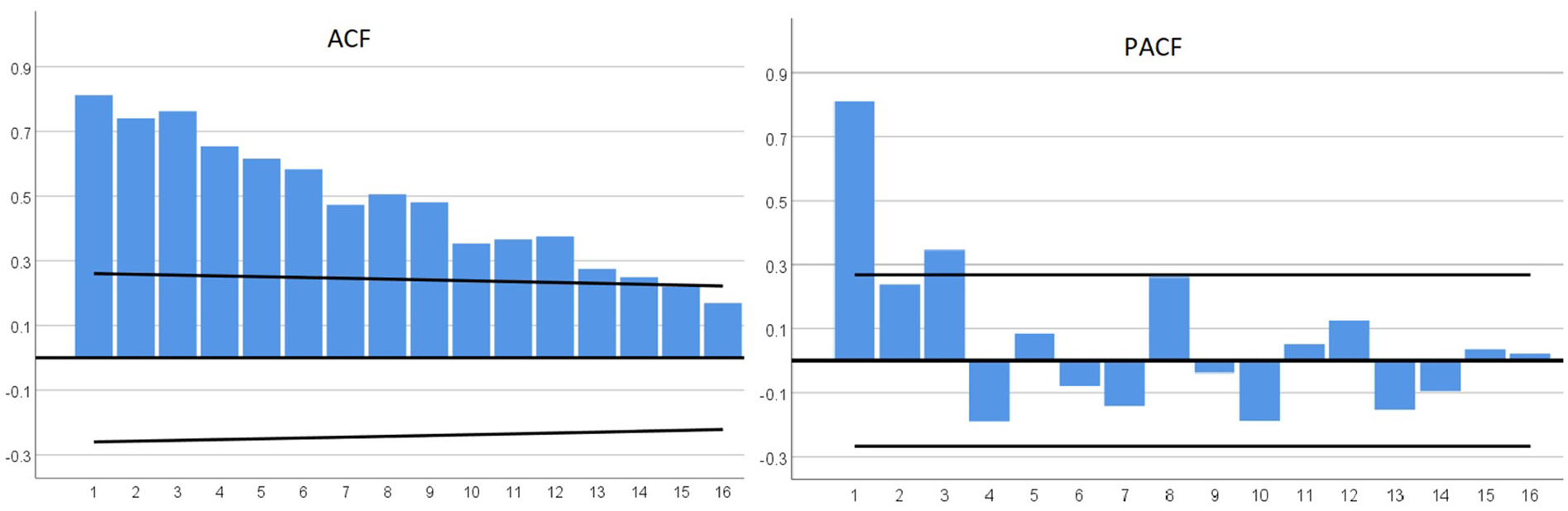We cannot conclude that a monthly seasonal pattern exists in the data set since $r_{12}$ is not significantly divergent from other lags, even if monthly data is used (Box et al., 2016). Both the unit root test and ACF/PACF pre-tests are consistent with each other; and also with the literature (Martins et al., 2021; Narins, 2017), considering the fact that the EV-demand data set contains periods from the introduction and into the subsequent growth periods of the EV-product life-cycle (see Figure 2).

Figure 1.

ACF and PACF coefficients of electric car demand (predicted variable).

Polynomial Regression

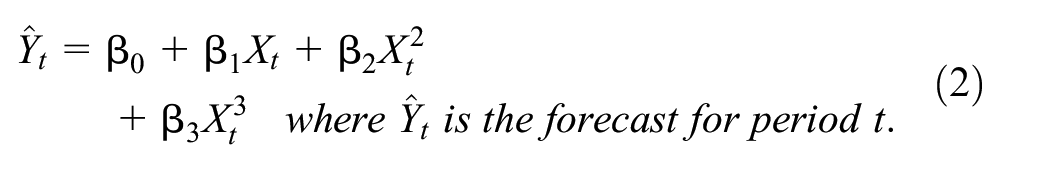
A min-max normalization is used in the polynomial regression, which responded better than the Z-score and square root methods. The polynomial order is determined with a training and validation split in order to alleviate overfitting risk. In-sample data points are divided into training and validation sets 100 times with the outer loop; and RMSE scores are calculated for the polynomial orders from one to six in the inner loop, since it is not expected to use an order higher than six, considering the data pattern presented with the blue line in Figure 2. The resulting RMSE scores are presented in Figure 3, in which the vertex point of the validation curve (red line) is obviously three. Therefore, a third-order polynomial is employed to forecast EV demand values (see Equation 2), which is consistent with the literature considering the low sample size of the present study (Bishop, 2006; James et al., 2021).

\begin{matrix} {\hat{Y}}_{t} = β_{0} + β_{1} X_{t} + β_{2} X_{t}^{2} \\ + β_{3} X_{t}^{3} where {\hat{Y}}_{t} is the forecast for period t . \end{matrix}

(2)

Figure 2.

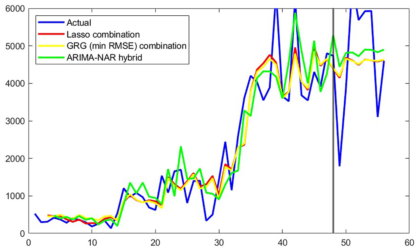
Best three forecasts versus actual electric car demand.

Figure 3.

RMSE scores of training/validation split for polynomial regression.

NAR

In-sample data points are divided into training and validation sets with 70% and 30%, respectively. A test set is not used, considering the quantity of data points. Two autoregressive components (feedback delay) are included in the input layer, and six neurons are used in the hidden one. Considering the low sample size, increasing the feedback delay, and hidden units increase the risk of overfitting (Bishop, 2006; James et al., 2021). First, the network is trained in a closed-loop structure, and in-sample period forecasts are obtained. MSE is minimized in validation to fit the network. Then, an open loop form is used to forecast out-of-sample.

{\hat{Y}}_{t} = h (Y_{t - 1}, Y_{t - 2})

(3)

Where the h-function is estimated with minimizing MSE; and feedback delays of $Y_{(t - 1)}$ and $Y_{(t - 1)}$ are autoregressive components to be included in the input layer of the neural network.

ARIMA

All explanatory variables listed in the methodology section were included in the ARIMA model with transfer functions; but none of them were significant, even with the confidence level reduced to 90%. Consequently, after trying multivariate, univariate, and seasonal and stationary ARIMA models, univariate ARIMA (3, 1, 1) produced the lowest error measures of all the tested ARIMA models (see Table 2 for model parameters). First-order differencing is used without any other transformation in the selected model; which is consistent with both the unit root test and autocorrelation results which indicate a trend pattern (Box et al., 2016). ARIMA forecast accuracy is better than NAR (see Tables 4 and 5) and all other singular forecast models similar to Kim et al. (2021) and G. P. Zhang (2003) and contradicting with Y. Wang et al. (2019). Moreover, the statistical model ARIMAs success over the machine learning and deep learning forecast models supports the findings of Makridakis et al. (2018); but runs counter to the results of Ahmed et al. (2010), since the former favors statistical models over machine learning but the latter suggests the opposite.

(1 - ϕ_{3} B^{3}) (1 - B) {\hat{Y}}_{t} = (1 + θ_{1} B) ϵ_{t}

(4)

where the differencing operator $(1 - B)^{d}$ indicates first-order differencing (d = 1), $(1 - ϕ_{3} B^{3})$ is the AR component including only a third order (p) component and $(1 + θ_{1} B)$ is the MA component of order (q) one.

Table 2.

ARIMA (3, 1, 1) Model Parameters.

Variable	Estimate	SE	t	Sig.
AR3 $(ϕ_{3})$	.430	.137	3.137	.003
MA1 $(θ_{1})$	.580	.125	4.621	.000

LSTM Deep Learning Neural Network

An RNN including an input layer, an LSTM layer with 128 hidden units, a dropout layer with 0.9 probability to alleviate the risk of overfitting, a fully connected layer, and a regression layer is designed for the process. The LSTM model is good for replicating the current patterns. However, this superior quality did not work for the benefit of the forecast presumably because of the extreme fluctuations at the end of in-sample periods. To lessen the effect of these extreme fluctuations on out-of-sample forecasts, the use of a less complex network is preferable. Additionally, considering its better in-sample forecasting performance and stronger statistical evidence of independent information, the NAR forecast is employed in the combination models, instead of the LSTM. However, it is worth noting that the success of the NAR and ARIMA models over the LSTM model in the present study (see Tables 4 and 5) runs counter to the findings of Fan et al. (2021) and Jiang et al. (2021), in which the LSTM model produced comparatively better accuracy measures.

Artificial Neural Networks (ANN)

The multivariate ANN model estimation uses randomly selected 70% of the in-sample data points for training and 30% of them for testing. An MLP network structure is used with three layers, where the first layer is for given explanatory variables; the second is the hidden one, with four neurons; and the third layer is the output. Predicted variable is normalized and explanatory variables are standardized before training of the network. The hyperbolic tangent activation function is used in the hidden layer. USD/TL currency rates, energy index, and livelihood index are the major determinants of EV demand in the ANN model.

Combination Forecasting

Each of the four different combining models employed in the present analysis includes forecasts from the best component models: NAR, ARIMA, and polynomial regression; which produced the best error measures of in-sample periods.

As a first step in this part of the analysis, our study conducts independent information tests by running in-sample regressions of realized values against predicted values of the component models using WLS (to overcome heteroscedasticity issues). If the estimated regression coefficients are nonzero and separately identified (which is the case in the present study), then the existence of independent information content in the component models is confirmed; and forming combinations of those respective component models forecasts may achieve superior forecast accuracy (Bates & Granger, 1969; Bischoff, 1989; Cooper & Nelson, 1975; Fair & Shiller, 1990; Nelson, 1972). Each of the component models processes the same time-series data differently, and is thus likely to contain different, independent information; with the ARIMA model reflecting linear functional relations of lagged predicted variables and residuals, the NAR model processing nonlinear functional relations nested in the time-series, and the polynomial regression modeling linear combinations of predicted variable and its powers. Our study then proceeds with forming combinations of the component model forecasts with four different approaches (as explained in the methodology section above) by employing: (a) A regression-based combining model (WLS); (b) a GRG algorithm combining model; (c) a LASSO-based combining model; (d) and a hybrid combining model.

Each of the four combining models of the present analysis utilizes forecasts from the best three component models: NAR, ARIMA, and polynomial regression. NAR is chosen over LSTM in the combining model as a source of independent information regarding nonlinear relations in the data, for two reasons. One, in a regression (in-sample) of actual values against predicted values, the NAR variable coefficient is significant, while the LSTM coefficient is not; which indicates that the NAR model contains independent information useful for combination forecasting (out-of-sample), while the LSTM model does not in the present study (Fair & Shiller, 1990). Two, because of the superior in-sample performance of the NAR variable over LSTM with regard to forecasting error; keeping in mind that machine learning methods suggest to act according to the training performance, on the grounds that parameters minimizing the training error will also minimize out-of-sample periods forecast error. This is so, because to avoid overfitting, trained model parameters are adjusted with a validation set, and the adjusted model is then examined with a test set.

Combining With WLS

With regard to the regression-based combining model (WLS), the estimated in-sample WLS regression coefficients (constrained to be nonnegative and to sum to one) serve as the weights assigned to each component forecast in the out-of-sample combination model. This particular constrained combining method led to improved forecast accuracy, in line with previous literature (Aksu & Gunter, 1992; Clemen & Winkler, 1986; Gunter, 1992; Gunter & Aksu, 1997; Nowotarski et al., 2014; Terregrossa, 2005; Terregrossa & Ibadi, 2021; Terregrossa & Sener, 2023).

Combining With GRG

With regard to the GRG-based combining model, our study employs a GRG algorithm to process in-sample data to estimate the component forecast weights for the out-of-sample combination forecast; with the estimated weights constrained to be nonnegative and to sum to one (Terregrossa & Sener, 2023). The GRG technique serves as one alternative to the more conventional approach of employing estimated in-sample regression coefficients as weights for combining forecasts. The GRG algorithm is employed for minimization purposes of nonlinear problems which makes it perfectly suitable for the combination forecast process. Additionally, GRG provides flexibility to minimize MAPE, RMSE, BIC, or any other error measures; while the WLS in-sample regression approach minimizes the SSE only, as does all regression-based approaches because the absolute value operator is not differentiable to minimize MAPE with the gradient descent. While minimizing RMSE and BIC for the combination models with GRG, both error measures produced equal component forecast weights which is expected. BIC is calculated as $BIC = - 2 loglikelihood + kln (n) = nln (MSE) + kln (n)$ where $n$ and $k$ represent the quantity of data points (56) and model parameters (3 + 1 = 4) respectively. Minimizing SSE, MSE, and RMSE are equivalent to each other and also equivalent to maximizing the logarithm of likelihood. Values of $n$ and $k$ behave as the constants of the BIC function so minimizing $\ln (MSE)$ is equivalent to minimizing RMSE because MSE is a nonnegative and monotonic function.

Combination forecast weights obtained with the constrained WLS and GRG approaches are presented in Table 3 for comparison. GRG combination forecasts are obtained with minimization of RMSE and MAPE respectively. The machine learning NAR model has the highest component forecast weight, which is consistent with previous literature (Terregrossa & Ibadi, 2021; Terregrossa & Sener, 2023). Our empirical findings also show that the combined model with GRG is better than its component models similar to the findings of Terregrossa and Sener (2023).

Table 3.

Combination Forecast Weights.

Component Forecasts	WLS	GRG minMAPE	GRG minRMSE
NAR	0.726	0.184	0.743
ARIMA	0.104	0.816	0.090
Poly Reg	0.170	0.000	0.167

Combining With LASSO

With regard to the third combination approach, LASSO regression is used to combine given component forecasts with the function given in Equation 4.1. In the LASSO-based approach component forecasts are normalized with the min-max method firstly; then possible terms for the function $X_{i}, X_{i}^{2}, X_{i}^{3}, X_{i}^{4}, \sqrt{X_{i}}, \ln X_{i}, \exp X_{i}, and reciprocal terms 1 / X_{i}, 1 / \exp X_{i}, 1 / \ln X_{i}$ are included into the function for the three component forecasts. The backward elimination approach is used in the beginning to reduce the number of terms. The given terms are used in three component forecasts or used in none of them. In the end $X_{i}, X_{i}^{2}, X_{i}^{3}, \sqrt{X_{i}}$ terms are selected for the equation presented in Equation 5 below.

Selected 12 series are re-normalized with the min-max method again. Then coefficients are estimated with cross-validation of 2-folds for 20 different lambda values descending from 15 with 0.9 rate. Results are presented in Figure 4 which presents the trade-off between over-fitting and under-fitting, where the green circle in the vertex shows the best lambda value of the combination model with respect to MSE. On the right side of the graph where lambda is close to zero, LASSO model uses all possible terms in the function below with very large coefficients while over-fitting the function. Contrarily, on the left side of the graph, higher lambda values force the absolute value of the sum of the coefficients to be close to zero with an under-fitted equation. The optimum lambda is estimated as 6.457 (12th one) in the vertex point between high variance (overfitting) and high bias (under-fitting) trade-off. Formula 1 presents the loss function of LASSO, where MSE is summed with the absolute value sum of the coefficients multiplied with lambda. The absolute value operator is not differentiable in all points so this part of the formula is not included in the gradient after differentiating the MSE component of the loss the function.

\begin{matrix} \hat{Y} = β_{0} + β_{1} C_{1} + β_{2} C_{1}^{2} + β_{3} C_{1}^{3} + β_{4} \sqrt{C_{1}} + β_{5} C_{2} + β_{6} C_{2}^{2} \\ + β_{7} C_{2}^{3} + β_{8} \sqrt{C_{2}} + β_{9} C_{3} + β_{10} C_{3}^{2} + β_{11} C_{3}^{3} + β_{12} \sqrt{C_{3}} \end{matrix}

(5)

where $C_{i}$ represents component forecast series NAR, ARIMA, and polynomial regression, respectively. Resulting nonzero coefficients are $B_{0} = 186.18, B_{1} = 3050.05, B_{2} = 402.04, B_{5} = 91.88, B_{7} = 341.38, B_{8} = 52.90 and B_{1} 2 = 968.77$ . The actual term $C_{i}$ and its square root are used twice, while its square and cube terms are used once. All three component forecasts carry independent information and contribute to the resulting function, but NAR has the highest impact which is consistent with the analysis regarding the WLS and GRG (min RMSE) combination models.

Figure 4.

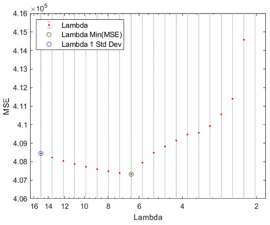
Cross validated MSE versus descending lambda values for LASSO.

Hybrid Forecasting

G. P. Zhang (2003) proposed that time-series data contain a linear autocorrelation pattern and a nonlinear component. ARIMA models the linear pattern; and its residuals contain the nonlinearity of the series. When ARIMA error is forecasted with nonlinear NAR, the residual prediction will be the forecast of the nonlinear component. Then, the ARIMA forecast and the NAR residual forecast is summed to combine linear and nonlinear components in order to reach the final forecast. ARIMA-NAR and NAR-ARIMA hybrid models improved forecast accuracy which is consistent with previous research of Kim et al. (2021); Sener et al. (2023); Y. Wang et al. (2019); G. P. Zhang (2003). On the other hand, the success of ARIMA over NAR is in line with Kim et al. (2021); G. P. Zhang (2003) but not with Y. Wang et al. (2019). The forecast results of the ARIMA-NAR hybrid model and its reverse, the NAR-ARIMA hybrid are presented in Tables 4 and 5 to compare its performance with the novel combinations approaches that we have proposed (GRG and LASSO). The LASSO-based combining model, the ARIMA-NAR hybrid model, and the GRG-based combining model (min RMSE) produced the best results in general.

Table 4.

In-sample Forecast Accuracy Measures.

				Component forecasts			Combination forecasts				Hybrid forecasts
Stats	LSTM	Damped Trend	ANN	NAR	ARIMA	Polynomialregression	WLS	GRGMAPE	GRG RMSE	LASSO	NAR ARIMA	ARIMA NAR
RMSE	836	781	619	587	732	752	571	680	571	566	576	631
MAPE	48.7%	56.5%	47.7%	43.0%	35.4%	45.8%	39.5%	34.0%	39.7%	36.2%	36.7%	38.2%
SMAPE	34.8%	39.9%	43.2%	33.2%	33.5%	32.9%	30.2%	31.0%	30.3%	27.5%	30.2%	31.8%
MAE	547	561	448	440	514	492	417	481	418	408	411	472
MPE	−34.5%	−37.1%	−10.2%	−24.3%	−7.5%	−21.7%	−21.7%	−9.4%	−21.9%	−18.2%	−18.4%	−19.7%
U1	0.167	0.154	0.121	0.112	0.144	0.148	0.110	0.132	0.110	0.108	0.110	0.118
U2	0.853	0.952	1.001	0.929	0.895	1.237	0.887	0.865	0.889	0.870	0.889	0.863

Table 5.

Out-of-sample Forecast Accuracy Measures.

				Component forecasts			Combination forecasts				Hybrid forecasts
Stats	LSTM	Damped trend	ANN	NAR	ARIMA	Polynomial regression	WLS	GRG	GRG	LASSO	NAR	ARIMA
Stats	LSTM	Damped trend	ANN	NAR	ARIMA	Polynomial regression	WLS	MAPE	RMSE	LASSO	ARIMA	NAR
RMSE	4,506	1,576	1,662	1,509	1,489	1,643	1,486	1,486	1,486	1477.2	1,490	1477.3
MAPE	113.9%	42.9%	39.5%	36.6%	39.2%	44.8%	37.5%	38.5%	37.4%	37.2%	36.5%	39.3%
SMAPE	64.8%	31.4%	34.6%	32.0%	31.02%	30.9%	31.0%	31.0%	31.0%	30.9%	31.7%	30.7%
MAE	4,180	1,357	1,483	1,365	1,327	1,340	1,323	1,325	1,323	1,318	1,352	1,312
MPE	−113.9%	−27.4%	−6.3%	−8.5%	−17.8%	−33.4%	−13.7%	−16.1%	−13.5%	−13.2%	−8.9%	−19.5%
U1	0.323	0.157	0.182	0.162	0.154	0.160	0.156	0.155	0.156	0.156	0.160	0.152
U2	1.866	0.572	0.563	0.549	0.548	0.633	0.542	0.545	0.542	0.546	0.538	0.545

Comparison of Forecast Errors

To begin, we take note that the studys forecast errors overall are rather high in general, with regard to both in-sample and out-of-sample test periods. This is likely due (at least in part) to the unstable nature of our data set, keeping in mind that EV-demand in Turkey is quite new and not yet stabilized, by any means. Moreover, approximately half of the data set is from unstable pandemic years. However, and nonetheless, within this particular framework of analysis, we can still discern relative, comparative performance among the models employed in the present study (Hanke & Wichern, 2014).

Comparison of Forecasts for In-sample Periods

In-sample forecast results, which are from first 48 periods of data for the years 2018 to 2021, are compared with respect to model fit statistics and presented in Table 4 below.

What stands out here is that the performance of the LASSO-based combining model appears to have dominated with regard to the in-sample analysis, in that the LASSO-based model produced the best measures for most of the error statistics: ranking first in five out of seven categories; and second in the remaining two.

Also noteworthy in this part of the analysis, is that all of the combination and hybrid models improved forecast accuracy over the component models forecasts, as mainly indicated by the SMAPE statistic. The MAPE statistic provides similar information, with one exception (the ARIMA model). Similarly, the squared error measures RMSE and Theils U1 and U2 (Armstrong & Collopy, 1992) also indicate that the combination and hybrid models generally provide better forecasts than the component models, with regard to the in-sample analysis.

U 1 = \sqrt{\frac{\sum_{t = 1}^{n - 1} {(Y_{t} - {\hat{Y}}_{t})}^{2}}{\sum_{t = 1}^{n} ({Y_{t}}^{2} - {\hat{Y}}_{t}^{2})}} U 2 = \sqrt{\frac{\sum_{t = 1}^{n - 1} {(\frac{Y_{t + 1} - {\hat{Y}}_{t + 1}}{Y_{t}})}^{2}}{\sum_{t = 1}^{n - 1} {(\frac{Y_{t + 1} - Y_{i}}{Y_{t}})}^{2}}}

(6)

Lastly, also of interest in this part of the study is that the two novel combination approaches in this paper (GRG-and LASSO-based) produced competitive results compared with the WLS-combination and the hybrid models.

Comparison of Forecasts for Out-of-sample Periods

The first 8 months of 2022 are selected as out-of-sample periods and are used for comparison of selected component and combination forecasts.

In this part of the analysis, the forecast accuracy measures generally indicate that all combination and hybrid models are successfully improved over the component models, as mainly indicated by the MAPE statistic. The LASSO-based model is generally the best among all combination models, and slightly better than the best hybrid, the ARIMA-NAR model (G. P. Zhang, 2003). In turn, the ARIMA-NAR hybrid performs better than its reverse, the NAR-ARIMA hybrid.

Also of interest is that the MAPE-minimizing GRG and RMSE-minimizing GRG combining models produced competitive results with the WLS regression-based combining model; with the min RMSE-GRG model performing slightly better.

Lastly, we note that the univariate models (NAR, ARIMA, damped trend, and polynomial regression) performed better than multivariate ANN, among component models tested in this part of the present analysis. LSTM model successfully replicates the pattern in the current data points while forecasting the future. However, this ability turned into a disadvantage because of the extreme fluctuations at the end of in-sample periods.

Forecast Comparison With Hypothesis Testing

The Diebold-Mariano (DM) test, DMs adapted version Harvey-Lewbourne-Newbold (HLN) test, the Wilcoxon signed rank test, and the sign test are all employed to discern whether significant differences exist for the given in-sample and out-of-sample forecasts (see Table 6). DM and HLN tests produced consistent results with each other, in general. Wilcoxon and sign tests did not detect any difference for out-of-sample periods; where the sample size is very small. Considering all test results, we can conclude that only LSTM is significantly different than others; indicating that the four combining models of the present analysis generated significantly better results compared to the NAR model. Considering the fact that combination and hybrid models do not show any statistically significant differences in forecast error, all of them can be accepted as successful models in a comparative sense.

Table 6.

Significances of Paired Comparison Tests for Out-of-sample Periods.

			Component forecasts			Combination forecasts				Hybrid forecasts
					Polynomial		GRG	GRG		NAR	ARIMA
Forecast models		LSTM	NAR	ARIMA	regression	WLS	MAPE	RMSE	LASSO	ARIMA	NAR
LSTM			0.07	0.12	0.33	0.09	0.12	0.09	0.09	0.07	0.12	Wilcoxon
LSTM			0.07	0.29	0.73	0.07	0.29	0.07	0.07	0.07	0.29	Sign
NAR	DM	0.00		0.78	1.00	0.78	0.67	0.78	0.44	0.40	0.67	Wilcoxon
NAR	HLN	0.00		1.00	1.00	0.73	0.73	0.73	0.73	0.73	1.00	Sign
ARIMA	DM	0.00	0.88		0.78	0.89	0.78	0.89	1.00	0.89	0.58	Wilcoxon
ARIMA	HLN	0.00	0.87		1.00	1.00	1.00	1.00	1.00	1.00	1.00	Sign
Polynomial	DM	0.10	0.67	0.44		0.58	0.78	0.58	0.58	0.89	0.58	Wilcoxon
Regression	HLN	0.12	0.66	0.44		1.00	1.00	1.00	1.00	1.00	1.00	Sign
WLS	DM	0.00	0.74	0.95	0.53		0.89	0.67	0.89	0.89	0.78	Wilcoxon
WLS	HLN	0.00	0.74	0.95	0.53		1.00	1.00	1.00	0.73	1.00	Sign
GRG MAPE	DM	0.00	0.83	0.90	0.48	0.99		0.89	0.89	0.78	0.67	Wilcoxon
GRG MAPE	HLN	0.00	0.82	0.90	0.48	0.99		1.00	1.00	0.73	1.00	Sign
GRG RMSE	DM	0.00	0.74	0.96	0.54	0.90	1.00		0.58	0.89	0.78	Wilcoxon
GRG RMSE	HLN	0.00	0.73	0.96	0.53	0.90	1.00		0.73	0.73	1.00	Sign
LASSO	DM	0.00	0.60	0.86	0.52	0.39	0.83	0.24		0.89	0.33	Wilcoxon
LASSO	HLN	0.00	0.60	0.86	0.52	0.39	0.83	0.25		1.00	0.29	Sign
NAR ARIMA	DM	0.00	1.00	1.00	0.63	0.96	0.98	0.66	0.84		0.78	Wilcoxon
NAR ARIMA	HLN	0.00	1.00	1.00	0.62	0.96	0.98	0.66	0.83		1.00	Sign
ARIMA NAR	DM	0.21	0.83	0.59	0.36	0.91	0.84	0.91	1.00	0.93
ARIMA NAR	HLN	0.22	0.83	0.59	0.36	0.91	0.84	0.91	1.00	0.93

Section Summary

The results section starts with unit root, breakpoint unit root, and ACF/PACF pre-tests of forecast models where they indicate a strong trend pattern for the EV-demand series. Then, polynomial regression, NAR, ARIMA, LSTM, ANN forecast models are presented. Polynomial regression, NAR, and ARIMA are selected as components for the combination and hybrid models. After that WLS, GRG, and proposed LASSO-based combination forecast models are compared with the ARIMA-NAR and NAR-ARIMA hybrid models. Comparisons are done with forecast accuracy measures as well as hypothesis testing.

Discussion

The present study tackles the research objective of improved forecast accuracy of the EV demand. Using only data available prior to an out-of-sample forecast horizon, the present study first generates simulated, ex-ante out-of-sample component model forecasts, employing classical statistical forecasting techniques as well as machine learning methods. Then four different combining methods are employed, to form simulated, ex-ante out-of-sample combinations of the different component model forecasts: (a) A conventional regression-based combining method (WLS) (Nowotarski et al., 2014; Terregrossa & Ibadi, 2021; Wu & Blake, 2023) that serves as a benchmark model, in which in-sample estimated regression coefficients serve as weights for the out-of-sample weighted average combination forecasts. (b) The relatively novel GRG combining approach (Terregrossa & Sener, 2023), in which a GRG technique is employed to estimate the component model forecast weights. With these first two combining methods, a shared conceptual idea is that by constraining the in-sample estimated forecast weights to be nonnegative and sum to one, greater efficiency is achieved in the weight-estimation process (in a statistical sense), resulting in greater accuracy of the out-of-sample combination forecasts. (c) An established hybrid combination model (ARIMA-NAR) (Kim et al., 2021; Y. Wang et al., 2019; G. P. Zhang, 2003;) in which an ARIMA model is employed to process any linear functional relations that may be contained in the data; and a NAR model is utilized to model the residuals from the ARIMA model, which will contain information about any nonlinear functional relations. The resultant combining model is then able to embody both linear and nonlinear relations that be inherent in the data. (d) Our study also introduces an original, novel combining method by forming a transcendental LASSO-function to combine forecasts generated by NAR, ARIMA, and polynomial regression models. When the underlying functional process inherent in the data is not known (which may be linear, nonlinear, or both), the inclusion of multiple elements to the combining model function increases the chance to recognize the true functional pattern; but may lead to overfitting. The overfitting problem is handled with LASSO optimization. Cross-validation and regularization are the critical success factors behind the LASSO-based technique to combine the component model forecasts.

In the out-of-sample testing part of the analysis, the forecast accuracy measures generally indicate that all combination and hybrid models are successfully improved over the component models, as mainly indicated by the mean absolute percentage error (MAPE) statistic. The LASSO-based model is generally the best among all combination models, and slightly better than the best hybrid model, the ARIMA-NAR model (G. P. Zhang, 2003), with regard to the different measures of forecast error.

According to our results, the ARIMA, NAR, and polynomial regression models are the best among the component forecast models; and all combination and hybrid models performed better than these component forecast models, both in sample and out of sample. The success of the ARIMA-NAR and NAR-ARIMA hybrid models over the component models is consistent with the findings of Kim et al. (2021), Y. Wang et al. (2019), and G. P. Zhang (2003). Although the forecasting precision of the ARIMA, NAR, and polynomial regression models over LSTM is not in line with the papers of Fan et al. (2021), and Jiang et al. (2021) (which find in favor of LSTM), the success of combination and hybrid models produced with them provides empirical support for their inclusion (see Tables 4 and 5). Our empirical results indicate that the LASSO-based combining model and the ARIMA-NAR hybrid are the two best-performing forecasting methods; followed by the RMSE-minimizing GRG-based and the WLS-regression-based combination models, respectively.

The two novel approaches proposed in this paper performed slightly better than reputable rivals for the given data set; which is evidence that the LASSO-based and GRG-based combination models can be employed as reliable alternatives to other combination and hybrid forecasting models. The GRG-based combining models are more practical and quick; whereas the LASSO-based combining model proves more effective but is computationally demanding. A comparison of forecast errors in Tables 4 and 5 indicates that the LASSO-based model generally performed the best among all combination models, and slightly better than the best hybrid, the ARIMA-NAR model G. P. Zhang (2003), in both in-sample and out-of-sample test periods for the given data set.

The major implications of our empirical findings are that greater accuracy in demand forecasting can be achieved with a combining model approach, rather than reliance on any particular, singular model. Furthermore, given its superior performance, the employment of the studys LASSO-based combining model to forecast EV-demand may lead to optimal firm decision-making over a range of organizational facets (see above), which is predicated on accurate demand function estimation.

Extreme fluctuations, especially toward the end of the in–sample periods of the EV-data set, and the low sample size are major limitations of the study.

Future research can entail analyses with larger data sets, in which the proposed LASSO-based combination model is expected to be more successful with higher model complexity without overfitting risk. With regard to a specific path of future research, outlier methodologies may be employed in formulating combination and hybrid forecasting models. See for example, Arslan (2012) and H. Wang et al. (2007); the former develops a combined least absolute deviation (LAD-LASSO) model that is resistant to heavy-tailed errors or outliers that are found in the responses; the latter study develops a combined weighted least absolute deviation (WLAD-LASSO) model that deals with heavy-tailed errors and outliers that are found in explanatory variables.

Table 7 below indicates the contribution of the present study in the evolutionary progression of the research field of combination forecast modeling. This table also serves as a broad guide, with respect to the path of future research in the field of study of combination forecasting.

Table 7.

Selected Combination Papers.

Bates and Granger (1969)	The genesis of the combination forecast concept with an exposition of various weighted average models; including OLS regression
Granger and Ramanathan (1984)	Regarding the case in favor of an unrestricted linear combination model including a constant term
Clemen (1986); Clemen and Winkler (1986)	Regarding the benefit of linear constraints on the combining model, in terms of the bias-efficiency tradeoff
Nowotarski et al. (2014)	Regarding constrained combining model regression and Bayesian model averaging
Diebold and Shin (2019)	Regarding the technique of a partially egalitarian LASSO for calculating combination weights
Dewangan et al. (2020)	Regarding combinations with support vector regression, graph valued regression, and deep networks
Terregrossa and Sener (2023)	Regarding the technique of a generalized reduced gradient algorithm (GRG) method for calculating combination forecast weights
(present study)	Regarding the employment of a transcendental LASSO function to generate a combination forecast

Conclusion

In the not-too-distant future, electric vehicles (EVs) will be replacing combustion-engine vehicles, helping to lower carbon emissions not only in economically developed nations but eventually in all nations across the globe. It is a matter of survival of the planet. Automobile manufacturers have already begun the manufacturing transition process, as is evident with the advent of hybrid vehicles; which will eventually make way to fully electric-powered vehicles, once an electric-power charging grid is well-established in each nation. As automobile manufacturers begin to make relevant production plans and corresponding input employment decisions, there is a clear need for accurate forecasts of EV demand.

The present analysis forecasts EV-demand with the use of a time series of demand data, which is shown to contain a trending pattern and at least one breakpoint with the employment of unit root, breakpoint unit root, and correlogram tests. As a result, the normalization methods of differencing, min-max, and Z-score are used in the different models of the study. After preprocessing, except for the ARIMA and damped-trend models, all component model forecasts were fitted with training and validation split; which resulted in successful improvements. The ANN model is fitted with a training/test split to compare similar measures in both sets before forecasting out of sample periods. The NAR and LSTM models are fitted with a training/validation split and are optimized to minimize the MSE of the validation set. The polynomial regression model order is determined by minimizing the RMSE score of the randomly selected validation data.

Forecast models trained with the in-sample data are applied to out-of-sample periods without using future information as input. Out-of-sample component forecasts are also combined with the weights estimated from in-sample periods. In other words, our all of the combination-model and the hybrid-model forecasts are simulated ex-ante forecasts, in the sense that they are generated only with the information available prior to an out-of-sample period.

After generating the component model forecasts (for both in-sample and out-of-sample test periods), our study constructs and employs four different combination forecast models; beginning with a regression-based model (WLS), in which estimated regression coefficients (in sample) serve as component model forecast weights to form combination forecasts (out of sample). After the conventional WLS approach to combine classical and machine learning forecasts, we employed two other, novel combining-model approaches to form combinations of NAR, ARIMA, and polynomial regression component forecasts: an GRG algorithm-based model; and a LASSO regression-based model. Combinations with the GRG-based approach are done alternately with minimizing MAPE and RMSE, respectively. We used component forecasts third-order polynomials plus a square root term as inputs in the LASSO-based combination model, which produced the best results compared with all models tested in the present analysis. We also employed two hybrid models of ARIMA-NAR and NAR-ARIMA, respectively, to help determine the comparative performance of the novel combination approaches. The LASSO-combining model produced the best overall results of all models tested, with regard to both in-sample and out-of-sample period testing.

Our empirical findings indicate that combination forecasting methodologies can be improved by using more complex approaches to combine component forecasts; as evidenced by the success of our transcendental LASSO-based combining approach (see Tables 4 and 5), over the method of computing weighted-averages of component models forecasts with GRG and WLS models.

Machine learning and deep learning models have been improving rapidly in the last decades. New multivariate sophisticated forecast models are also candidates for combining approaches with their versatile nature, as is the case with the LASSO model. For instance, deep learning LSTM neural networks and convolutional neural networks (CNN) are invented for different purposes but they have been used for forecasting and they can be implemented for combining forecasts in future studies.

Footnotes

Copyright Statement

Copyright

Rules of use

This class file is made available for use by authors who wish to prepare an article for publication in a SAGE Publications journal. The user may not exploit any part of the class file commercially.

This class file is provided on an as is basis, without warranties of any kind, either express or implied, including but not limited to warranties of title, or implied warranties of merchantablility or fitness for a particular purpose. There will be no duty on the author[s] of the software or SAGE Publications Ltd to correct any errors or defects in the software. Any statutory rights you may have remain unaffected by your acceptance of these rules of use.

Declaration of Conflicting Interests

The author(s) declared no potential conflicts of interest with respect to the research, authorship, and/or publication of this article.

Funding

The author(s) received no financial support for the research, authorship, and/or publication of this article.

ORCID iDs

Uğur Şener

Salvatore Joseph Terregrossa

Data Availability Statement

The data set of the paper can be downloaded from the relevant institutions of Turkey (odmd.org.tr, tcmb.gov.tr, ) and corresponding author can help for any inconvenience.

References

Aburto

Weber

(2007). Improved supply chain management based on hybrid demand forecasts. Applied Soft Computing Journal, 7, 136–144. https://doi.org/10.1016/j.asoc.2005.06.001

Ahmed

N. K.

Atiya

A. F.

Gayar

N. E.

El-Shishiny

(2010). An empirical comparison of machine learning models for time series forecasting. Econometric Reviews, 29(5–6), 594–621.

Aksu

Gunter

S. I

. (1992). An empirical analysis of the accuracy of SA, OLS, ERLS and NRLS combination forecasts. International Journal of Forecasting, 8(1), 27–43.

Altenburg

Corrocher

Malerba

(2022). China’s leapfrogging in electromobility. A story of green transformation driving catch-up and competitive advantage. Technological Forecasting and Social Change, 183, 121914.

Amiri

Heidari

Navimipour

N. J.

Unal

(2023a). Resilient and dependability management in distributed environments: A systematic and comprehensive literature review. Cluster Computing, 26(2), 1565–1600.

Amiri

Heidari

Navimipour

N. J.

Unal

Mousavi

(2023b). Adventures in data analysis: A systematic review of deep learning techniques for pattern recognition in cyber-physicalsocial systems. Multimedia Tools and Applications, 83, 1–65.

Armstrong

J. S.

Collopy

(1992). Error measures for generalizing about forecasting methods: Empirical comparisons. International Journal of Forecasting, 8(1), 69–80.

Arslan

(2012). Weighted lad-lasso method for robust parameter estimation and variable selection in regression. Computational Statistics & Data Analysis, 56(6), 1952–1965.

Bates

J. M.

Granger

C. W. J.

(1969). The combination of forecasts. Operational Research Society, 20, 451–468. https://www.jstor.org/stable/3008764

10.

Bischoff

C. W.

(1989). The combination of macroeconomic forecasts. Journal of Forecasting, Vat, 8, 293–314.

11.

Bishop

C. M.

(2006). Pattern recognition and machine learning. Springer Science+Business Media, LLC.

12.

Bodunrin

M. O.

(2020). Flow stress prediction using hyperbolic-sine arrhenius constants optimised by simple generalised reduced gradient refinement. Journal of Materials Research and Technology, 9, 2376–2386. https://doi.org/10.1016/j.jmrt.2019.12.070

13.

Box

G. E.

Jenkins

G. M.

Reinsel

G. C.

Ljung

G. M.

(2016). Time series analysis forecasting and control. (5th ed.). Wiley. ISBN 9781118675021.

14.

Broadbent

G. H.

Allen

C. I.

Wiedmann

Metternicht

G. I.

(2022). Accelerating electric vehicle uptake: Modelling public policy options on prices and infrastructure. Transportation Research Part A: Policy and Practice, 162, 155–174.

15.

Charniak

. (2019). An introduction to deep learning. MIT Press.

16.

Chen

. (2011a). Chinese automobile demand prediction based on ARIMA model. In 2011 4th International Conference on Biomedical Engineering and Informatics (BMEI) (Vol. 4, pp. 2197–2201). IEEE.

17.

Chen

K. Y.

(2011b). Combining linear and nonlinear model in forecasting tourism demand. Expert Systems with Applications, 38, 10368–10376. https://doi.org/10.1016/j.eswa.2011.02.049

18.

Chen

Zhao

. (2010, August). Demand forecasting in automotive aftermarket based on ARMA model. In 2010 international conference on management and service science (pp. 1–4). IEEE.

19.

Chiang

C. Y

Lin

W. T.

Suresh

N. C.

(2016). An empirically-simulated investigation of the impact of demand forecasting on the bullwhip effect: Evidence from us auto industry. International Journal of Production Economics, 177, 53–65.

20.

Clemen

R. T.

(1986). Linear constraints and the efficiency of combined forecasts. Journal of Forecasting, 5(1), 31–38.

21.

Clemen

R. T.

Winkler

R. L.

(1986). Combining economic forecasts. Journal of Business & Economic Statistics, 4(1), 39–46.

22.

Cooper

J. P.

Nelson

C. R.

(1975). The ex ante prediction performance of the st. louis and frb-mitpenn econometric models and some results on composite predictors. Journal of Money, Credit and Banking, 7, 1–32. https://about.jstor.org/terms

23.

Dewangan

C. L.

Singh

Chakrabarti

(2020). Combining forecasts of day-ahead solar power. Energy, 202, 117743. https://doi.org/10.1016/j.energy.2020.117743

24.

Diebold

F. X.

(2015). Comparing predictive accuracy, twenty years later: A personal perspective on the use and abuse of dieboldmariano tests. Journal of Business and Economic Statistics, 33, 37–41. https://doi.org/10.1080/07350015.2014.983236

25.

Diebold

F. X.

Mariano

R. S.

(1995). Comparing predictive accuracy. Journal of Business & Economic Statistics, 13, 134–144. https://doi.org/10.1016/0169-2070(88)90124-0

26.

Diebold

F. X.

Shin

(2019). Machine learning for regularized survey forecast combination: Partially-egalitarian lasso and its derivatives. International Journal of Forecasting, 35(4), 1679–1691. https://doi.org/10.1016/j.ijforecast.2018.09.006

27.

Dolgui

Pashkevich

(2009). Forecasting demand for slow-moving items in case of reporting errors. Risk and Decision Analysis, 1, 221–230. https://doi.org/10.3233/RDA-2009-0019

28.

Ebrahimi

Salamzadeh

Soleimani

Mohammad

S. K.

Zarea

Fekete-Farkas

(2022). Startups and consumer purchase behavior: Application of support vector machine algorithm. Big Data and Cognitive Computing, 6(2), 34.

29.

Fair

Shiller

(1990). Comparing information in forecasts from econometric models. The American Economic Review, 80, 375–389.

30.

Fan

Sun

Yao

Zhang

Yan

Sun

(2021). Well production forecasting based on arima-lstm model considering manual operations. Energy, 220, 119708.

31.

Fattah

Ezzine

Aman

El Moussami

Lachhab

(2018). Forecasting of demand using ARIMA model. International Journal of Engineering Business Management, 10, 1847979018808673.

32.

Goodfellow

Bengio

Courville

(2016). Deep learning. MIT press.

33.

Granger

C. W. J.

Ramanathan

(1984). Improved methods of combining forecasts. Journal of Forecasting, 3, 197–204. https://doi.org/10.1002/for.3980030207

34.

Gunter

S. I.

(1992). Nonnegativity restricted least squares combinations. International Journal of Forecasting, 8(1), 45–59.

35.

Gunter

S. I.

Aksu

(1997). The usefulness of heuristic n(e)rls algorithms for combining forecasts. Journal of Forecasting, 16, 439–462. https://doi.org/10.1002/(sici)1099-131x(199711)16:6<439::aid-for624>3.0.co;2-8

36.

Gutierrez

R. S.

Solis

A. O.

Mukhopadhyay

(2008). Lumpy demand forecasting using neural networks. International Journal of Production Economics, 111, 409–420. https://doi.org/10.1016/j.ijpe.2007.01.007

37.

Haghani

Sprei

Kazemzadeh

Shahhoseini

Aghaei

(2023). Trends in electric vehicles research. Transportation Research Part D: Transport and Environment, 123, 103881.

38.

Hanke

J. E.

Wichern

D. W.

(2014). Business forecasting. (9th ed.). Pearson. ISBN 9780132301206.

39.

Harvey

Leybourne

Newbold

(1997). Testing the equality of prediction mean squared errors. International Journal of Forecasting, 13, 281–291.

40.

Hochreiter

Schmidhuber

(1997). Long short-term memory. Neural Computation, 9(8), 1735–1780.

41.

Hsieh

M. C.

Giloni

Hurvich

(2020). The propagation and identification of arma demand under simple exponential smoothing: Forecasting expertise and information sharing. IMA Journal of Management Mathematics, 31, 307–344. https://doi.org/10.1093/imaman/dpaa006

42.

Huang

Gao

(2023). Forecasting bitcoin futures: A lasso-bma two-step predictor selection for investment and hedging strategies. SAGE Open, 13(1), 21582440231151652.

43.

Iwan

Nürnberg

J. M.

Kijewska

(2021). Efficiency of light electric vehicles in M, last mile deliveries–szczecin case study. Sustainable Cities and Society, 74, 103167.

44.

James

Witten

Hastie

Tibshirani

(2021). An introduction to statistical learning. (2nd ed.). Springer. http://www.springer.com/series/417

45.

Jiang

Liu

Niu

Zhang

(2021). A combined forecasting system based on statistical method, artificial neural networks, and deep learning methods for short-term wind speed forecasting. Energy, 217, 119361.

46.

Kim

Choi

C. Y.

Shahandashti

Ryu

K. R.

(2021). Improving accuracy in predicting city-level construction cost indices by combining linear arima and nonlinear anns. Journal of Management in Engineering, 38, 04021093. https://doi.org/10.1061/(asce)me.1943-5479.0001008

47.

Kochak

Sharma

(2015). Demand forecasting using neural network for supply chain management. International Journal of Mechanical Engineering and Robotics Research, 4(1), 96–104. www.ijmerr.com

48.

Lasdon

Fox

Ratner

(1974). Nonlinear optimization using the generalized reduced gradient method. RAIRO-Operations Research-Recherche Oprationnelle, 3, 73–103.

49.

Dai

(2020). Bitcoin price forecasting method based on cnn-lstm hybrid neural network model. The Journal of Engineering, 2020(13), 344–347.

50.

D. W.

Cao

(2010). A unified synchronization criterion for impulsive dynamical networks. Automatica, 46, 1215–1221. https://doi.org/10.1016/j.automatica.2010.04.005

51.

Makridakis

Spiliotis

Assimakopoulos

(2018). Statistical and machine learning forecasting methods: Concerns and ways forward. PLOS ONE, 13(3), e0194889.

52.

Martins

L. S.

Guimarães

L. F.

Junior

A. B. B.

Tenório

J. A. S.

Espinosa

D. C. R.

(2021). Electric car battery: LF, Junior ABB, An overview on global demand, recycling and future approaches toward sustainability. Journal of Environmental Management, 295, 113091.

53.

Mitrea

C. A.

Lee

C. K. M.

(2009). A comparison between neural networks and traditional forecasting methods: A case study. International Journal of Engineering Business Management, 1, 11.

54.

Mulema

S. A.

Garca

A. C.

(2018). Quality and productivity in aquaculture: Prediction of oreochromis mossambicus growth using a transfer function arima model. International Journal for Quality Research, 12, 823–834. https://doi.org/10.18421/IJQR12.04-03

55.

Murphy

K. P.

(2022). Probabilistic machine learning an introduction (1st ed.). The MIT Press.

56.

Mustaffa

A. S.

Shabri

. (2020, August). An improved rolling NGBM (1, 1) forecasting model with GRG nonlinear method of optimization for fossil carbon dioxide emissions in Malaysia and Singapore. In 2020 11th IEEE control and system graduate research colloquium (ICSGRC) (pp. 32–37). IEEE.

57.

Nahmias

Tava

(2015). Production and operation analysis. (7th ed.). Waveland Press.

58.

Narins

T. P.

(2017). The battery business: Lithium availability and the growth of the global electric car industry. The Extractive Industries and Society, 4(2), 321–328.

59.

Nelson

(1972). The prediction performance of the frb-mit-penn model of the U.S. economy. American Economic Association, 62, 902–917.

60.

Nowotarski

Raviv

Trck

Weron

(2014). An empirical comparison of alternative schemes for combining electricity spot price forecasts. Energy Economics, 46, 395–412. https://doi.org/10.1016/j.eneco.2014.07.014

61.

Patel

M. M.

Tanwar

Gupta

Kumar

(2020). A deep learning-based cryptocurrency price prediction scheme for financial institutions. Journal of Information Security and Applications, 55, 102583.

62.

Rahman

Herdiani

E. T.

Islamiyati

(2023). Application of nonparametric sign and wilcoxon sign rank control charts on animal feed data of pt. japfa comfeed indonesia, tbk. Application of nonparametric sign and Wilcoxon sign rank control charts on animal feed data of PT. Japfa Comfeed Indonesia, Tbk, 131(1), 4.

63.

Reiner

Fichtinger

(2009). Demand forecasting for supply processes in consideration of pricing and market information. International Journal of Production Economics, 118, 55–62. https://doi.org/10.1016/j.ijpe.2008.08.009

64.

Rodrigues

Cardeira

Calado

Melicio

(2017). Family houses energy consumption forecast tools for smart grid management. Controlo, 2016, 402. http://link.springer.com/10.1007/978-3-319-43671-5

65.

Roanec

J. M.

Kai

Krjanc

Fortuna

Mladeni

(2021). Automotive oem demand forecasting: A comparative study of forecasting algorithms and strategies. Applied Sciences, 11, 6787. https://doi.org/10.3390/app11156787

66.

Salamzadeh

Ebrahimi

Soleimani

Fekete-Farkas

(2022). Grocery apps and consumer purchase behavior: Application of gaussian mixture model and multi-layer perceptron algorithm. Journal of Risk and Financial Management, 15(10), 424.

67.

Sener

(2015). Trkiye’de binek otomobili endstrisinin talebine kantitatif bir yaklam. http://acikarsiv.aydin.edu.tr/bitstream/11547/1875/1/391630.pdf

68.

Sener

Kilic

B. I.

Tokgozlu

Zafer

(2023). Prediction of wind speed by using machine learning. In International conference on computational science and its applications (pp. 73–86). Springer.

69.

Sharifi

A. M.

Khalili Damghani

Abdi

Sardar

(2022). A hybrid model for predicting bitcoin price using machine learning and metaheuristic algorithms. Journal of Applied Research on Industrial Engineering, 9(1), 134–150.

70.

Taalbi

Nielsen

(2021). The role of energy infrastructure in shaping early adoption of electric and gasoline cars. Nature Energy, 6(10), 970–976.

71.

Terregrossa

S. J.

(2005). On the efficacy of constraints on the linear combination forecast model. Applied Economics Letters, 12, 19–28. https://doi.org/10.1080/1350485042000307062

72.

Terregrossa

S. J.

Ibadi

M. H.

(2021). Combining housing price forecasts generated separately by hedonic and artificial neural network models. Asian Journal of Economics, Business and Accounting, 21, 130–148. https://doi.org/10.9734/ajeba/2021/v21i130345

73.

Terregrossa

S. J.

Sener

(2023). Employing a generalized reduced gradient algorithm method to form combinations of steel price forecasts generated separately by arima-tf and ann models. Cogent Economics and Finance, 11, 2169997. https://doi.org/10.1080/23322039.2023.2169997

74.

Tibshirani

(1996). Regression shrinkage and selection via the lasso. Journal of the Royal Statistical Society: Series B (Methodological), 58, 267–288. https://doi.org/10.1111/j.2517-6161.1996.tb02080.x

75.

Uras

Marchesi

Tonelli

(2020). Forecasting bitcoin closing price series using linear regression and neural networks models. PeerJ Computer Science, 6, e279.

76.

Wang

F. K.

Chang

K. K.

Tzeng

C. W.

(2011). Using adaptive network-based fuzzy inference system to forecast automobile sales. Expert Systems with Applications, 38, 10587–10593. https://doi.org/10.1016/j.eswa.2011.02.100

77.

Wang

Jiang

(2007). Robust regression shrinkage and consistent variable selection through the lad-lasso. Journal of Business & Economic Statistics, 25(3), 347–355.

78.

Wang

Chen

Yang

(2015). Analyzing and predicting heterogeneous customer preferences in Chinas auto market using choice modeling and network analysis. SAE International Journal of Materials and Manufacturing, 8, 668–677. https://doi.org/10.4271/2015-01-0468

79.

Wang

(2021). The prediction of gold futures prices at the shanghai futures exchange based on the meemd-cs-elman model. SAGE Open, 11(1), 21582440211001866.

80.

Wang

Yuan

(2019). Seasonality and trend prediction of scarlet fever incidence in mainland china from 2004 to 2018 using a hybrid sarima-narx model. PeerJ, 7, e6165.

81.

Blake

(2023). The impact of the covid-19 crisis on air travel demand: Some evidence from China. Sage Open, 13(1), 21582440231152444.

82.

Zhang

Patuwo

B. E.

M. Y.

(1998). Forecasting with artificial neural networks: The state of the art. International Journal of Forecasting, 14, 35–62. https://doi.org/10.1016/S0169-2070(97)00044-7

83.

Zhang

G. P.

(2003). Time series forecasting using a hybrid arima and neural network model. Neurocomputing, 50, 159–175. www.elsevier.com/locate/neucom

84.

Zhang

G. P.

(ed.). (2004). Neural networks in business forecasting. IGI global.

85.

Zhang

Jiang

Cai

Huang

Chen

(2023). Transport-environmental kuznets curve hypothesis: Evidence from belt and road. SAGE Open, 13(2), 21582440231177873.

86.

Zhang

. (ed.). (2008). Artificial higher order neural networks for economics and business. IGI Global.

A Transcendental LASSO Function for Combining Machine Learning and Statistical Model Forecasts

Abstract

Keywords

Introduction

Literature

Section Summary

Methodology

Results

Data Set

Unit root test and Correlogram (ACF/PACF)

Polynomial Regression

NAR

ARIMA

LSTM Deep Learning Neural Network

Artificial Neural Networks (ANN)

Combination Forecasting

Combining With WLS

Combining With GRG

Combining With LASSO

Hybrid Forecasting

Comparison of Forecast Errors

Comparison of Forecasts for In-sample Periods

Comparison of Forecasts for Out-of-sample Periods

Forecast Comparison With Hypothesis Testing

Section Summary

Discussion

Conclusion

Footnotes

Copyright Statement

Declaration of Conflicting Interests

Funding

ORCID iDs

Data Availability Statement

References