Sage Journals: Discover world-class research

Abstract

Predicting operational performance enables organizations to develop operational effectiveness goals considering different combinations of resources. Measuring performance is consolidated with advances in relative efficiency analysis techniques, including data envelopment analysis (DEA) and stochastic frontier analysis (SFA), albeit these methods lack predictive capability. This paper proposes an approach for performance prediction by integrating relative efficiency measurement models with machine learning algorithms. Data analyses were conducted using data provided by the energy assessment project offered to small and medium-sized manufacturing companies in the United States (n 7,548) using sales as the output, with the inputs being the number of employees, hours of operation, electricity, natural gas, cost of electricity, and cost of natural gas. Performance was estimated differently, employing parametric (SFA) and non-parametric (DEA) methods. The prediction benchmarking process occurred by adopting machine learning algorithms: regression (LM), support vector machine (SVM), K-nearest neighbor (KNN), linear discriminant analysis (LDA), random forest (RF), and decision tree (DT). The findings showed that it is possible to identify the best prediction algorithm associated with a performance model. However, the performance prediction may differ if different strategies for measuring performance or machine learning model configurations are used. In addition, SFA-LOG and SVM had the best performance for regression, and DEA-VRS/IRS excelled with random forest; the RF algorithm was the best fit across all performance approaches. The error rate depends on the algorithm and the performance model, and the number of classes must be reduced to obtain a higher success rate.

Plain language summary

Predicting operational performance enables organizations to develop operational effectiveness goals by considering different combinations of resources. Companies that incorporate more accurate forecast models into their strategies can have a competitive advantage in the market, mainly by delivering the product to the right place, in the exact quantity, and at the right price. Given this context, there is a need to test new models and their combinations to achieve better results. This paper proposes an approach for performance prediction by integrating relative efficiency measurement models with machine learning algorithms. To test the prediction models, data analyses were conducted using data from the energy assessment project offered to small and medium-sized manufacturing companies in the United States (n 7,548). The findings showed that it is possible to identify the best prediction algorithm associated with a performance model. However, the performance prediction may differ if different strategies for measuring performance or machine learning model configurations are used. The error rate depends on the algorithm and the performance model, and the number of classes must be reduced to obtain a higher success rate. One of the main contributions of this article is that it demonstrates that the prediction performance can differ if distinct strategies to measure performance or configuration of the model are used. The results showed that it is possible to identify the best prediction algorithm associated with a given model performance.

Keywords

data envelopment analysis stochastic frontier analysis machine learning industrial energy performance forecasting

Introduction

Given the exponential growth and complexity of the managerial hierarchy (Cameli, 2023), new forms of management, such as continuous improvement processes and competitiveness (K. S. Wang, 2013), have emerged in the literature, especially after the advance of globalization to leverage resources (Czinkota & Ronkainen, 2005; Kwok & Arpan, 2002). This wave has generated the need for organizations to increasingly monitor performance at all stages of producing goods and services (Chandler, 1977; Neely, 1999; Shin et al., 2022). In this context, performance measurement systems have become vital for organizations to maintain a competitive advantage in the market (Gerhardt et al., 2021).

Numerous performance measurement systems have become important at strategic and operational levels (Bach et al., 2019; Danese & Kalchschmidt, 2011; A. D. Neely, 1999; Vegter et al., 2023). Performance measurement can be defined as “the process of quantifying the efficiency and effectiveness of action” (A. Neely et al., 1995, p. 4), with efficiency being an ex-post measure that shows how managers have solved different optimization issues, and effectiveness being an ex-ant measure that provides a goal for solving problems (Mariano, 2007; O’Donnell, 2018). According to Mariano (2007, p. 3), “an efficient system does not necessarily need to be effective and vice versa, meaning that the goal set can diverge from the maximum value on the optimization curve.”

The problem with effectiveness is that it relies on a utility function U(.) unknown beforehand. This problem was overcome by applying Farrell’s (1957) efficiency concept, shifting the focus from effectiveness to relative efficiency. Among the techniques for measuring relative efficiency, two stand out: stochastic frontier analysis (SFA) and data envelopment analysis (DEA); the first technique originates in econometrics and the second in mathematical programming (Bogetof & Otto, 2010a,b). The agents involved in this process are generally called decision-making units (DMU). Traditional relative efficiency analysis techniques such as DEA and SFA have limitations in terms of predictive capability. One of the problems of these techniques, which has been recognized throughout the literature, is that they have no predictive ability, meaning that a new model must be developed to encompass a new case (Dalvand et al., 2014; Hong et al., 1999; Kwon, 2017; Zhu et al., 2021).

Predicting operational performance for organizations to develop operational effectiveness goals is important. One of the primary importance of implementing a predicting operational performance is that it enables the organization to develop strategies and effectiveness targets considering different combinations of resources (inputs) (X. Wang et al., 2022). Accurate predicting also enables sensitivity analyses, allowing one to know the impact on the performance of marginal input changes (Yen et al., 2021). Establishing the importance of each input and output to performance is another competitive advantage (Puchalsky et al., 2018).

Research has demonstrated that the best-performing prediction models meet the needs of organizations, improving accuracy and service level (fill rate) for superior alignment of production capacity in meeting demands. In fact, evidence has shown that operational decisions can be based on prediction (da Veiga et al., 2016). Hence, manufacturing companies should consider prediction a necessary process to direct production activities (Danese & Kalchschmidt, 2011). To this end, prediction models are expected to be parsimonious, with few parameters, lower implementation costs, and adjust an organization’s prediction performance to achieve better results (Agostino et al., 2020; da Veiga et al., 2016).

Given this context and the need and importance of performance prediction (Kourentzes et al., 2019), this paper proposes an approach for performance prediction using machine learning (ML). Machine learning methods have been well explored in recent decades and have shown promising results, especially in helping solve prediction problems. Despite providing relevant results, there is still a need to further investigate new approaches and non-linear applications to improve performance prediction (Mariani et al., 2019). In the proposed method, different performance models are predicted by various ML algorithms to find the prediction with the lowest error rate associated with each performance model. Thus, in order to validate and test the model in an empirical study and provide practical evidence, the proposed experiment was performed with information from the North American energy assessment project for the industrial sector and involved small and medium-sized companies (SMEs).

This study’s results indicate that a systematized approach that integrates performance models SFA and DEA with machine learning algorithms has yet to be developed. The findings shed light on the literature through insights into the realized experiments. Energy performance prediction can create a higher learning environment for decision-making.

Materials and Methods

Systematic Literature Review

To justify the need for this study and this paper’s originality, it was necessary to first conduct a systematic literature review to identify the research gap that addresses the approach for performance prediction that considers different models, such as SFA, DEA, and a benchmarking process of predictive models. Therefore, the review was conducted to identify papers that specifically address performance prediction using relative efficiency analysis techniques. To this end, this review proposed to uncover which performance models were used, which prediction algorithms were adopted, how the features and targets were set up in the prediction, and what were types of problems modeled (Table 1 and Figure 1).

Table 1.

Papers on Performance Prediction.

Authors	Country	Journal/conference	Model	Algorithm	Attributes	Target	Problem
Hong et al. (1999)	South Korea	Expert Systems with Applications	AED*	Decision tree, self-organizing maps	Inputs and outputs	Efficiency (DEA tier)	Classification
Rezaie et al., 2013	Iran, Malaysia	World Applied Sciences Journal	AED	Support vector machines	Inputs and outputs	Efficiency (continuous)	Regression
Dalvand et al. (2014)	Iran	Advances in Environmental Biology	AED	Decision tree	Inputs and outputs	Efficiency (ten classes)	Classification
Gupta et al. (2016)	India	1st IEEE International Conference	DEA-CRS	Nearest Neighbor, Logistic Regression, Support Vector Machines	Inputs and outputs	Efficiency (two classes)	Classification
Kwon (2017)	USA	International Journal of Production Economics	DEA-CCR	Artificial neural network	Inputs and outputs	Efficiency (continuous)	Regression
Tsolas et al. (2020)	Greece, United Kingdom	Expert Systems with Applications	DEA (CRS-VRS-NIRS-NDRS)	Artificial neural network	Inputs and outputs	Efficiency (four classes)	Classification
Nandy and Singh (2020)	India	Journal of Cleaner Production	AED-VRS	Random Forest and Logistic Regression	Environment Variables	Efficiency (two classes)	Classification
Zhu et al. (2021)	China, United Kingdom	Journal of Management Science and Engineering	DEA-CCR	Neural Network, Genetic Algorithm and Support Vector Machines	Inputs and outputs	Efficiency (continuous)	Classification

Note. *AED Attention mechanism enabled post-model Explanation with Density peaks clustering algorithm for synonyms search and substitution (Liu et al. 2023).

Figure 1.

Approach for performance prediction.

The papers were selected using the search string (TITLE-ABS-KEY (“machine learning” OR “artificial intelligence” OR “deep learning”)) AND (TITLE-ABS-KEY (“data envelopment analysis” OR “stochastic frontier analysis”)) and searched on the Web of Science (WoS) and Scopus databases with no time limit. The selection criteria for the papers were based on the abstract (ABS), keywords (KEY), and title (TITLE), with no other filter added. The database search was performed in March/2020 and updated on 06/May/2021, and 196 papers were found in Scopus and 118 in WoS. After analyzing the titles and abstracts, 20 articles were selected for full-text analysis, and eight met the initial search protocol (Table 1).

Table 1 lists previous papers that analyzed research corroborating this article. For instance, Hong et al. (1999) was the first one identified and cited 41 times in the Scopus database. Recent interest in the topic stands out, with five papers published between 2017 and 2021. The second study was cited 21 times (Kwon, 2017), followed by the more recent studies of Nandy and Singh (2020) and Tsolas et al. (2020), with five and six citations, respectively. Despite the number of papers in WoS and Scopus, many cover the joint use of performance/efficiency and ML techniques. Still, the main goal is not prediction, thereby reinforcing the novelty and originality of this paper.

Approach to Performance Prediction

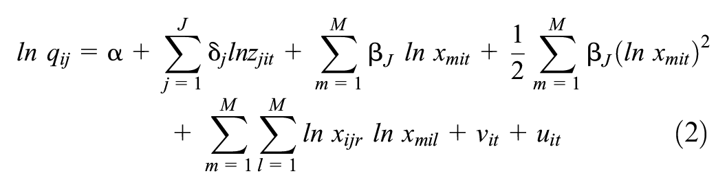
The literature showed that DEA and SFA propose to identify the efficient frontier (performance) so that on the frontier will be the equally efficient cases relative to the others. The SFA is a parametric (econometric) technique that estimates the stochastic frontier, assuming random residuals. The SFA was developed simultaneously by Aigner et al. (1977) and Meeusen and van Den Broeck (1977) and can be represented mathematically in Cobb-Douglas and translog forms by Equations 1 and 2, respectively, where q is the output, z is possible environment variables, x is the inputs, v is the error, and u is the inefficiency. The SFA is estimated by the maximum likelihood principle (O’Donnell, 2018).

\ln q_{1 it} = α + \sum_{j = 1}^{J} δ_{j} {lnz}_{jit} + \sum_{m = 1}^{M} β_{j} {lnx}_{mit} + v_{it} + u_{it}

(1)

l n q_{i j} = α + \sum_{j = 1}^{J} δ_{j} l n z_{j i t} + \sum_{m = 1}^{M} β_{J} l n x_{m i t} + \frac{1}{2} \sum_{m = 1}^{M} β_{J} {(l n x_{m i t})}^{2} + \sum_{m = 1}^{M} \sum_{l = 1}^{M} l n x_{i j r} l n x_{m i l} + v_{i t} + u_{i t}

(2)

The DEA is used to determine the efficiency frontier via mathematical programming (i.e., non-parametric). It was developed by Charnes et al. (1978) as a minimization (input-oriented) problem (Equation 3), where: $x_{ij} - x_{i 0}$ are the inputs/inputs under evaluation, $- y_{rj} - y_{r 0}$ are the outputs/outputs under evaluation, $θ$ is the efficiency, and $λ_{j}$ is the coefficient. It is also possible to develop the maximization problem (output-oriented). The advantage of DEA lies in its flexibility, and it can even be modeled in spreadsheets (Zhu, 2014).

| \begin{matrix} θ^{*} = \min θ, sujeito a & CRS : \sum_{J = 1}^{n} λ_{j} \geq 0 \\ \sum_{j = 1}^{n} λ_{j} x_{ij} \leq θ x_{i 0 i = 1, 2, \dots, m;} & VRS : \sum_{J = 1}^{n} λ_{j} \geq 1 \\ \sum_{j = 1}^{n} λ_{j} y_{rj} \geq y_{r 0 r = 1, 2, \dots, s;} & IRS : \sum_{J = 1}^{n} λ_{j} \leq 0 \\ λ_{j} \geq 0 & DRS : \sum_{J = 1}^{n} λ_{j} \geq 1 \end{matrix} |

(3)

The differences in performance estimation come from the multiple alternatives for the modeling. One of the first challenges in prediction is that there is a range of possible models. For instance, SFA can be estimated in Cobb-Douglas, quadratic, cubic, and other forms, whereas DEA can be input or output oriented as well as assume different assumptions for the return to scale, as shown in Equation 3: constant (CRS), variable (VRS), increasing (IRS), and decreasing (DRS). Some models even combine both approaches, such as stochastic non-smooth envelopment of data (StoNED; M. Andor & Hess, 2014; M. A. Andor et al., 2019; Bogetof & Otto, 2010a,b; O’Donnell, 2018).

The second challenge refers to a significant amount of learning algorithms. As a limitation of this study, the interest in the proposed application lies in the supervised algorithms, as the goal is to predict a continuous or categorical target. The systemic literature review performed herein presents some of these algorithms in Table 1. It is important to note that machine learning libraries, including “mlr3”and “scikit-learn,” implement dozens of learners that are ready to be configured and used (Becker et al., 2022; Grus, 2016; James et al., 2013; Müller & Guido, 2017).

This paper aims to develop an approach integrating models with predictive algorithms; to this end, was adopted the definition of a predictive model of Provost and Fawcett (2016, p. 45): “A predictive model is a formula for estimating the unknown value of interest: the target. The formula can be mathematical or it can be a logical statement, such as a rule.” In summary, learning a predictive model is done in a training process in which the data is randomly divided into training and test samples. This can be just two samples, training and testing (holdout) or cross validation with multiple samples for training and testing (cross validation; Becker et al., 2022).

The Model

Based on the results found in the systematic literature review, the characteristics of the performance models (DEA and SFA) and the training process of the predictive algorithms, this paper proposes an approach for performance prediction (Figure 1). The following steps were developed for this: (a) performance (efficiency) estimation is done through parametric and non-parametric models. After the estimation, (b) the inputs and outputs enter as attributes, and the performance (efficiency) enters as the variable to be predicted (target) in the predictive modeling. The target variable should be put on the same scale (normalized between 0 and 1) for comparison purposes. Different discretization strategies can be implemented for ranking, such as simple split, probabilistic, cluster, or sliced/tiered DEA. Notably, Hong et al. (1999) introduced the notion of DEA tiers as a strategy to identify similar DMUs. In practice, this method identifies all production functions in a data set, forming clusters.

In addition to outputs and inputs, environmental variables can enter as explanatory attributes in the prediction model depending on the outcome. Various environmental turbulences in the market can impact the production of goods and services in an organization (Chatterjee et al., 2023). This phenomenon has been thoroughly investigated over the decades (Ansoff, 1979, Duncan, 1972; Feng et al., 2021; Marzall et al., 2022). These authors corroborated the literature by demonstrating how unexpected environmental changes cause some organizations to thrive and others not. Managers cannot control environmental variables in the market environment, including technological, natural, political, economic, demographic, and cultural variables (Kotler & Keller, 2012; O’Donnell, 2018). Hence, it is imperative to highlight that some predictive models achieve superior results when data are placed on the same scale considering environmental issues (i.e., normalized or standardized) (Müller & Guido, 2017), with a better configuration of variables and attributes.

After setting up attributes and the target variable, the data is divided into training and testing (different strategies exist) and submitted to different prediction and classification algorithms in a benchmarking process. It is a complex task to determine a priori which algorithm will best fit the data; therefore, training should be conducted with several supervised algorithms, and it is mathematically complex to treat each algorithm. Nonetheless, algorithms can be classified into three types: those that (a) fit a mathematical model to the data (regression [LM], support vector machine [SVM]), those (b) based on similarity (K-nearest neighbor [KNN], linear discriminant analysis [LDA]), and lastly, those (c) that can present information gain (random forest [RF] and decision tree [DT]), among others (Provost & Fawcett, 2016).

Linear regression is one of the best-known algorithms and primarily aims to estimate a vector of parameters $β$ and a constant $α$ that shows the relationship between a dependent variable y and one or more independent variables x: $y_{i} = α + β_{1} x_{i 1} + \dots + β_{k} x_{ik} + ε_{1}$ . Support Vector Machine is a linear discriminant with a complex mathematical approach that creates a hyperplane between nearby data points, allowing one to marginalize the classes and maximize the distances between the points to better differentiate them (Vapnik, 1998). For KNN, given a positive interval K and an observation $x_{0}$ , the algorithm first identifies the K points in the training data that are near $x_{0}$ , represented by $N_{0}$ . It then estimates the conditional probability for class j as the fraction of points in $N_{0}$ , whose response values are equal to j: $\Pr ({Y = j | X = x}_{0}) \frac{1}{k} \sum_{i \in N_{0}} I (y_{i} = j)$ (An et al., 2021). In LDA, firstly, one calculates the mean of each class and the total mean $(μ_{i}, μ) : μ_{i} = \frac{1}{n_{j}} \sum_{x_{i} \in ω_{j}} x_{i} e μ = \frac{1}{N} \sum_{i = 1}^{N} x_{i} = \sum_{i = 1}^{c} \frac{n_{i}}{N} μ_{i}$ considering a set of N samples $[x_{i}]_{i = 1}^{N}$ . The matrix between classes is then calculated $S_{B} (MxM)$ : $S_{B} = \sum_{j = 1}^{c} n_{i} (μ_{i} - μ) (μ_{i} - μ)^{T}$ , and finally, the matrix within the class $S_{w} (MxM)$ : $S_{w} = \sum_{j = 1}^{c} \sum_{i = 1}^{n_{j}} (x_{ij} - μ_{j}) (x_{ij} - μ_{j})^{T}$ . The decision tree considers information gain and is based on a purity measure called entropy, where each $p_{i}$ is the probability of the property $i$ within the set, which ranges from $p_{i} = 1$ when all members of the set have the property $i$ , and $p_{i} = 0$ when no member of the set has the property $i$ : $entropia = - p_{1} \log (p_{1}) - p_{2} \log (p_{2}) \dots - p_{n} \log (p_{n})$ (Zhou et al., 2023). Random forest is based on decision trees, although they create a forest of trees where the outcome is determined by the votes in the formations. The approach in Figure 1 shows that other algorithms can be adopted, since some libraries have as many as 100+ learners, and many are possible (Grus, 2016; James et al., 2013; Provost & Fawcett, 2016; Tharwat et al., 2017).

Notably, the proposed prediction approach has two necessary feedback processes in case the prediction result is not satisfactory. The first indicates that environmental variables can be used as additional attributes (Figure 1, left side). The extreme case of Nandy and Singh (2020) used only environment variables (Table 1). The feedback on the right side of Figure 1 is related to three considerations in performance modeling: (a) the need for redesign, (b) the use of a new model, and (c) the combination of models. The combination of performance models is not new in the literature; for instance, Azadh et al. (2009) combined parametric and non-parametric modeling through geometric mean, while M. A. Andor et al. (2019) employed both mean and maximum value between DEA and SFA.

The packages “scikit-learn” (https://scikit-learn.org/) and “mlr3” (https://mlr3.mlr-org.com/) have tools (pipelines) that facilitate benchmarking these algorithms (Lang et al., 2019). These tools also provide a series of metrics for evaluation, and in the regression problem, the most commonly used ones are: (a) mean absolute error (MAE), (b) root mean square error (RMSE), and (c) bias. The classification includes (a) accuracy, (b) classification error, and (c) accuracy and recall. The final process is the choice of the algorithm(s) with the best result.

The result of the algorithm(s) can still be improved by hyperparameter tuning before the final approach is chosen. Optimization is a process that automatically tests many parameters of the algorithms. For example, the number of neighbors and trees are the main hyperparameters of the KNN and random tree algorithms, respectively.

Data Collection and Processing

In order to develop the application, the sample comprised the energy assessment project offered to small and medium-sized manufacturing companies in the United States. This sample was selected given its relevance and scope. The project is one of the largest in the world in this modality and involves over 30 American universities and almost 20,000 assessments. The sample and the data evaluated are available on the website (https://iac.university/). For the final version of the proposed model, this study employed the data downloaded on 04/29/2021, totaling 19,491 assessments from 1981 to 2020. The main limitation of the selected data is related to its processing, and other authors have also reported this issue (Abadie et al., 2012; Anderson & Newell, 2004).

Since DEA is sensitive to extreme values, the data were treated using the “tidyverse” package of the R environment. The analyses included (a) manufacturing firms with ≥50 employees, (b) firms with >2,000 hr of annual operations, (c) >1,000 (kWh) annual energy use, and (d) >$10,000 in sales, since obscure sales data were identified. Some missing data were also excluded, so the sample consisted of 11,883 assessments, which is still a considerable number. Not all DEA models ran properly even after the data treatments, and an outlier detection process was adopted. Based on the literature, it was necessary to apply the box-plot method; with this, the final sample consisted of 7,548 assessments. This is considered a large sample for DEA modeling and not feasible for spreadsheet processing. The solution was to use the R environment, which is the most viable option for the proposed case.

Results: Application Development

After various tests, the variables (a) sales (SALES) as the output and employees (EMPLOYEES), use of (b) electricity in kWh (USAGE_ELEC), use of (c) natural gas in MMBtu (USAGE_NAT), (d) cost of electricity (COST_ELEC), (e) cost of natural gas (COST_NAT), and (f) operational hours (PRODHOURS) were selected for the inputs (inputs). Table 2 lists the descriptive statistics of the data. It is worth noting that the restrictions regarding using natural gas were not added. Therefore, it is indicated that the minimum value of $ 38.00 refers to a manufacturing company that uses little of this resource, despite its considerable size for a small company, with up to 50 employees.

Table 2.

Summary of the Annual Data of the 7,548 Assessed Manufacturing Companies.

Statistics	Sales (u$)	Employees	Usage_elec (kWh)	Usage_nat (mmbtu)	Prodhours	Cost_elec (u$)	Cost_nat (u$)
Minimum	10,000.00	50	2,478	1,001	2,008	3,581.00	38.00
1st quartile	10,000,000.00	50	1,417,937	3,524	3,840	79,091.00	20,507.00
Median	20,000,000.00	125	2,635,991	8,152	5,000	141,915.00	44,906.00
Mean	26,577,000.00	152.6	3,522,434	1,3647	5,121	180,750.00	65,478.00
3rd quartile	35,000,000.00	200	3,522,434	18,571	6,240	249,485.00	93,794.00
Maximum	113,000,000.00	460	17,146,886	77,212	8,763	602,507.00	249,817.00

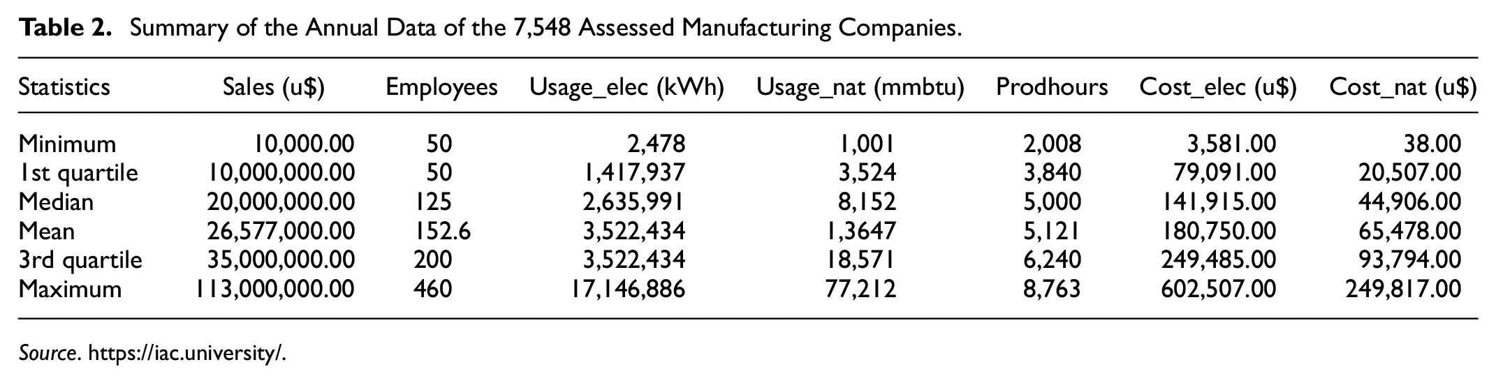
Source. https://iac.university/.

Estimating the energy performance models was done in the “Benchmarking” and “Frontier” packages of R, developed by researchers at the Copenhagen Business School (CBS) and the University of Queensland in Australia (Bogetoft & Otto, 2020; Coelli & Henningsen, 2020). The performance of the 7,548 manufacturing firms was calculated in six different ways, where one assumes four returns in the DEA to scale: (a) constant (CRS), (b) variable (VRS), (c) increasing (IRS), (d) decreasing (DRS), and two functional forms are used in SFA: (a) log-linear (SFA-LOG) and (b) quadratic in logarithms (SFA-TRANSLOG). Figure 2 shows the coding developed in R on Google Colab, which is a cloud environment for code execution created in Google Suite (Figure 3).

Figure 2.

Coding for the performance/efficiency models.

Figure 3.

Colab environment.

The result is presented in Figure 4 through the frequency distribution. One can observe the similarity in the distribution of the SFA models and between the returns to scale: VRS and IRS and CRS and DRS. The first point is whether the performance can be predicted using the inputs and outputs for the attributes. The second point is to know how the machine learning algorithms fit the different performance models. It is worth noting that this is an important contribution to the proposed model.

Figure 4.

Frequency distribution of energy performance models.

As illustrated in Figure 1, both regression and classification models can be used by adopting either a continuous or discrete scale. In Figure 5, the continuous scale TGH is the target variable for the regression problem, and the discrete scale TGH_cat is the prediction objective in classification.

Figure 5.

Coding for continuous and discrete scaling.

For the proposed prediction model, six learning algorithms were selected. The algorithms were selected based on their popularity, applicability, and agreement with the literature in Table 1 and Figure 1. The algorithms were KNN, LM, LDA, RF, DT, and SVM.

For the benchmarking process, the k-fold cross-validation strategy was implemented, and after various tests, k = 5 were selected, where the data is partitioned into five parts called folds. Sequences of models are trained so that each part is used in training and testing, ensuring greater stability to the process (Müller & Guido, 2017). For regression, the main comparison metric was a mean square error (MSE), and for classification, the accuracy. For this, modeling was performed in “mlr3” (R environment) and “scikit-learn” (Python) using Google Colab; “mlr3” was selected for its convenience in the benchmarking process. The regression coding and classification are detailed in Figures 6 and 7.

Figure 6.

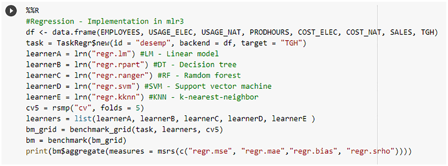
Coding for benchmarking algorithms for regression.

Figure 7.

Coding for benchmarking algorithms for classification.

Table 3 lists the RMSE of the algorithms for the six regression approach performance models. The darkest blue represents the best result (lowest error), and the red color represents the worst result (highest error). The best fit occurs with the SVM on the SFA-LOG model. However, the algorithm that adapted best to all models was RF, and the worst was LM. The algorithms were configured with the same parameters to compare model performance (Table 3).

Table 3.

Regression Approach for Energy Performance Prediction.

Note. Hyperparameters: KNN (K = 7); RF (num.trees = 500; alpha = 0.5); DT (minsplit = 20; cp = 0.01; maxdepth = 30); SVM (kernel = radial). The values given in bold likely indicate the best performance for each model across the different regression methods (KNN, LM, RF, DT, SVM). These bold values represent the lowest error rates or best predictive accuracy achieved by the corresponding model-method combination. For example: For the DEA-CRS model, the bold value under the RF method (0.001105) suggests that this combination achieved the best performance among all methods tested for DEA-CRS. Similarly, for the SFA-LOG model, the bold value under the SVM method (0.000919) indicates the best performance for this model. This boldface highlighting helps quickly identify the most effective regression method for each model in terms of minimizing prediction error or maximizing prediction accuracy.

Learning by classification is not as simple as regression since the performance generated in Figure 4 is continuous and not categorical. For discretization, it was necessary to use an unsupervised method available in the “arules” package, implementing the strategy of intervals of the same size (Hahsler et al., 2011; Figure 5). Another method used was stratification using sliced DEA (DEA-TIER), which was first presented by Hong et al. (1999). The latter is a supervised method for identifying performance clusters. Since no package was identified in R to train this process, a custom function had to be built in R (Figure 8). Since this is a supervised technique, choosing the number of clusters is impossible. For the 7,548 manufacturing firms, the function identified 15 to 20 clusters, depending on the return to scale, which were regrouped by performance level to match the number of classes in the analysis.

Figure 8.

Function for training the DEA-TIER.

Table 4 lists the accuracy of the five algorithms for the six performance models using the two discretization strategies for DEA (tier and non-tier) and organized with classes of four sizes (2, 3, 5, and 10), generating 200 comparisons. In this case, in the overall context, the best algorithms are also RF and SVM, with the best result being in the RF with the DEA-IRS and DEA-VRS models. This study found that the prediction model’s performance worsens considerably as more classes are aggregated. Nonetheless, the interval strategy showed superior results when compared to the tier method, although the construction of the latter is much more complex.

Table 4.

Classification Approach for Predicting Energy Performance.

Source. Research data.

Note. Hyperparameters: KNN (K = 7); RF (num.trees = 500; alpha = 0.5); DT (minsplit = 20; cp = 0.01; maxdepth = 30); SVM (kernel = radial).The bold values indicate the best model.

An important issue regarding classification is the limitation of the accuracy metric for unbalanced data, as is the case for DEA-CRS (Figure 4). Two other metrics that capture the behavior in each class are accuracy and recall, and that in the first, it is possible to identify the proportion of false negatives (FN = 1-recall), and in the second, the proportion of false positives (FP = 1-accuracy), present in each class, a result corroborated by Müller and Guido (2017). Another issue that is not limited to classification is the optimization of the hyperparameters. Given this, the following examples were highlighted to work with the optimization approach for RF since this algorithm presented the best result for classification. The coding of the hyperparameter identification is illustrated in Figure 9, and the training is shown in Figure 10. To generate the confusion matrix (with the test data), the holdout strategy was used.

Figure 9.

Identification of the best hyperparameters for the random forest.

Figure 10.

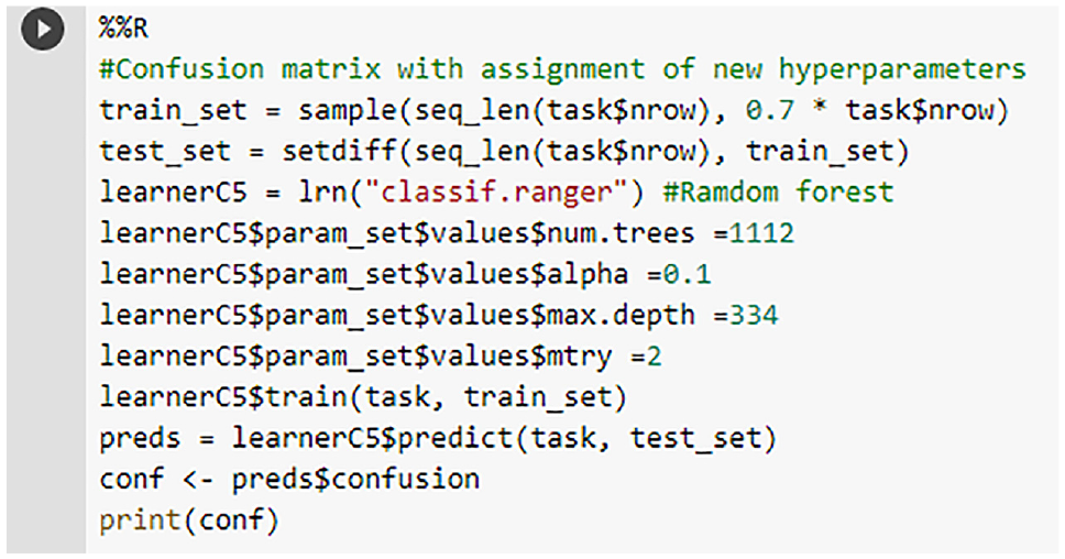
Training the model and generating the confusion matrix.

Table 5 lists the confusion matrix of the DEA-VRS model using the RF algorithm to predict five classes, where “A” represents the best energy performance and “E” is the worst. In this case, there is no disproportionality between false positives and negatives, as the classes are relatively balanced. The accuracy was 97% using the holdout method (slightly higher than the result in Table 4). In Table 6, the same procedure was performed for 10 classes. Although class D has a higher proportion of false negatives, it does not represent an outlier. Therefore, accuracy was 93%, with no significant improvement over Table 4.

Table 5.

Confusion Matrix for RF-DEA-VRS Prediction (Five Classes).

Classes	E	D	C	B	A	Real	Recall	FN
E	476	10	0	1	0	487	0.98	2%
D	5	633	13	1	2	654	0.97	3%
C	0	4	311	8	1	324	0.96	4%
B	0	0	2	323	10	335	0.96	4%
A	0	0	0	5	460	465	0.99	1%
Accuracy	0.99	0.98	0.95	0.96	0.97	2,265
FP	1%	2%	5%	4%	3%

Source. Prepared by the authors using the R package “mlr3.”

Note. Optimized hyperparameters: (num.trees = 1,112; alpha = 0,1; max.depth = 334; mtry = 2)—Accuracy: 97%.The boldface values highlight the correct predictions for each class.

Table 6.

Confusion Matrix for RF-DEA-VRS Prediction (10 Classes).

Class	J	I	H	G	F	E	D	C	B	A	Real	Recall	FN
J	102	6	0	0	0	0	0	0	0	0	108	0.94	6%
I	9	328	12	0	0	1	0	0	1	2	353	0.93	7%
H	0	3	298	19	1	0	0	0	0	1	322	0.93	7%
G	0	0	12	342	15	4	0	0	0	1	374	0.91	9%
F	0	0	0	1	129	5	1	0	0	1	137	0.94	6%
E	0	0	0	0	2	169	8	1	1	1	182	0.93	7%
D	0	0	0	0	0	7	101	6	3	1	118	0.86	14%
C	0	0	0	0	0	0	2	173	7	2	184	0.94	6%
B	0	0	0	0	0	0	0	5	185	10	200	0.93	8%
A	0	0	0	0	0	0	0	0	5	282	287	0.98	2%
Accuracy	0.92	0.97	0.93	0.94	0.88	0.91	0.90	0.94	0.92	0.94	2,265
FP	8%	3%	7%	6%	12%	9%	10%	6%	8%	6%

Source. Prepared by the authors using the R package “mlr3.”

Note. Optimized hyperparameters: (num.trees = 1,667; alpha = 0,1; max.depth = 500; mtry = 3)—Accuracy: 93%.The boldface values highlight the correct predictions for each class.

The confusion matrix in Table 7 uses the DEA-CRS to predict ten classes, and the result differs from the previous ones. This occurred because the classes were unbalanced, and the error reached 100% for class B; the accuracy was 87% (i.e., a little better than the result using the cross-validation strategy).

Table 7.

Confusion Matrix for RF-DEA-CRS Prediction (10 Classes).

Class	J	I	H	G	F	E	D	C	B	A	Real	Recall	FN
J	762	30	0	0	0	0	0	0	0	0	792	0.96	4%
I	38	756	55	0	0	0	0	0	0	0	849	0.89	11%
H	0	18	291	32	1	1	0	0	0	1	344	0.85	15%
G	0	0	17	97	27	1	0	0	1	0	143	0.68	32%
F	0	0	0	11	43	17	2	0	0	0	73	0.59	41%
E	0	0	0	0	4	16	5	1	2	0	28	0.57	43%
D	0	0	0	0	0	5	7	2	1	2	17	0.41	59%
C	0	0	0	0	0	0	1	2	1	2	6	0.33	67%
B	0	0	0	0	0	0	0	0	0	2	2	0.00	100%
A	0	0	0	0	0	0	1	0	3	7	11	0.64	36%
Accuracy	0.95	0.94	0.80	0.69	0.57	0.40	0.44	0.40	0.00	0.50	2,265
FP	5%	6%	20%	31%	43%	60%	56%	60%	100%	50%

Source. Prepared by the authors using the R package “mlr3.”

Note. Optimized hyperparameters: (num.trees = 556; alpha = 0,60; max.depth = 500; mtry = 4)—Accuracy: 87%.The boldface values highlight the correct predictions for each class.

Final Considerations

This paper shows that a systematized approach that integrates performance models (SFA and DEA) with machine learning algorithms has not yet been developed, although the results shed light on the literature in various ways and key findings. The first finding of this paper is related to (a) the need for a broader approach involving various performance models and ML algorithms; (b) it shows that the literature has not yet considered SFA in performance prediction; (c) it is in line with the introduction of efficiency scaling that enables the comparison of different models (e.g., DEA, SFA, input, and output-oriented models). The fourth finding lies in (d) different discretization forms that can be used, such as interval, frequency, probability, and clustering, and lastly, (e) the fifth insight highlights benchmarking in two stages within the model and between models.

The proposition of a new prediction model in the literature is a complex topic, and this study did not seek to exhaust the possibilities suggested in the proposed approach for industrial energy performance prediction modeling presented herein. Nevertheless, one of the main contributions of this article lies in the fact that it demonstrates that the prediction performance can differ if distinct strategies to measure performance or configuration of the ML model are used. The results showed that it is possible to identify the best prediction algorithm associated with a given model performance, as suggested in Figure 1. Moreover, SFA-LOG and SVM performed best for regression, and DEA-VRS/IRS stood out with random forest. In fact, the RF algorithm was the best fit across all performance approaches.

In terms of classifying the best-performing prediction model, the results in Table 4 demonstrate that as the number of classes increases, the error grows considerably, as the error rate was found to rely on both the algorithm and the model performance. One must decrease the number of classes to obtain a higher success rate. The results in Table 7 also confirm such a need if the number of classes is unbalanced. In the latter case, a change of strategy for performance measurement (efficiency) may be necessary. The key point is that the highest proportion of false positives and negatives occur in adjacent classes.

In the context of Industry 4.0, the performance prediction approach (classification or regression) can be useful for companies, since it can be incorporated into business intelligence systems and into the equipment itself from an Internet of Things perspective. The possibility of energy performance prediction can create a higher learning environment for decision-making. Since the approach implements learning algorithms that typically perform better as more data is trained, it is emphasized that implementing this approach requires organizations to have a data-driven culture. In light of this, it is believed that failure to develop such a culture may be an obstacle to making this modeling work in organizations.

Even in the face of several contributions, this article has limitations that need to be observed. The first limitation is the single database. In this context, exploring databases of other types of companies is necessary to generalize the results. Another limitation is in the forecasting process, which is uncertain by nature. Testing new techniques and parameter adjustments is crucial for better accuracy. Given this, future studies are suggested to test new performance models and the constructs that combine parametric and non-parametric modeling. Another possibility for future research is to adopt the simulation procedure for model selection proposed by M. A. Andor et al. (2019) to verify if the models with the best-predicting results have the best success indicators of actual inefficiency since these methods share the same metrics for outcome evaluation. Predicting is complex, and this study did not intend to exhaust the subject. Therefore, new studies are needed, especially for empirical work based on evidence, and to test new models to assist managers and decision-makers in various organizations, whether for-profit or not-for-profit, public or private.

Footnotes

Acknowledgements

The authors wish to express their gratitude to the Editor and Anonymous reviewers for their constructive input and kind feedback. Also, thanks to Fundação Dom Cabral (FDC) for financial support for the publication of this article.

Declaration of Conflicting Interests

The author(s) declared no potential conflicts of interest with respect to the research, authorship, and/or publication of this article.

Funding

The author(s) disclosed receipt of the following financial support for the research, authorship, and/or publication of this article: The authors Veiga and Silva thank the National Council for Scientific and Technological Development—CNPq (Grants number: 312023/2022-7-PQ and 302407/2022-7 PQ) for its financial support of this work.

Fundação Dom Cabral—The APC was funded by FDC.

Ethical Approval

No applied.

Informed Consent Statement

Informed consent was obtained from all subjects involved in the study.

ORCID iD

Claudimar Pereira da Veiga

Data Availability Statement

Support data may be requested from the corresponding author.

References

Abadie

L. M.

Ortiz

R. A.

Galarraga

(2012). Determinants of energy efficiency investments in the US. Energy Policy, 45, 551–566.

Agostino

I. R. S.

da Silva

W. V.

Pereira da Veiga

Souza

A. M.

(2020). Forecasting models in the manufacturing processes and operations management: Systematic literature review. Journal of Forecasting, 39, 1043–1056. https://doi.org/10.1002/for.2674

Aigner

Lovell

C. K.

Schmidt

(1977). Formulation and estimation of stochastic frontier production function models. Journal of Econometrics, 6(1), 21–37.

Wang

Guo

(2022). Data reduction based on NN-kNN measure for NN classification and regression. International Journal of Machine Learning and Cybernetics, 13(3), 765–781. https://doi.org/10.1007/s13042-021-01327-3

Anderson

S. T.

Newell

R. G.

(2004). Information programs for technology adoption: The case of energy-efficiency audits. Resource and Energy Economics, 26(1), 27–50.

Andor

M. A.

Parmeter

Sommer

(2019). Combining uncertainty with uncertainty to get certainty? Efficiency analysis for regulation purposes. European Journal of Operational Research, 274(1), 240–252.

Andor

Hesse

(2014). The StoNED age: The departure into a new era of efficiency analysis? A Monte Carlo comparison of StoNED and the “oldies” (SFA and DEA). Journal of Productivity Analysis, 41(1), 85–109.

Ansoff

(1979). Strategic management. Palgrave Macmillan.

Azadeh

Ghaderi

S. F.

Sohrabkhani

(2009). A simulated-based optimization approach for parametric modeling of electrical energy consumption. Energy, 34(9), 1437–1447.

10.

Becker

Martin Binder

Bischl

Burk

Casalicchio

Dandl

Fischer

Foss

Kotthoff

Lang

Pfisterer

Pulatov

Schneider

Schratz

Sonabend

Thomas

Wright

M. N.

(2022). mlr3 book. Retrieved December 20, from https://mlr3book.mlr-org.com/

11.

Bach

T. M.

Dalazen

L. L.

da Silva

W. V.

Ferraresi

A. A.

da Veiga

C. P.

(2019). Relationship between innovation and performance in private companies: Systematic literature review. SAGE Open, 9(2). https://doi.org/10.1177/2158244019855847

12.

Bogetoft

Otto

(2010a). Benchmarking with DEA and SFA, R package version 0.29. https://CRAN.R-Project.org/package=Benchmarking

13.

Bogetoft

Otto

(2010b). Benchmarking with DEA, SFA, and R: 157. Springer Science & Business Media.

14.

Bogetoft

Otto

(2020). Benchmarking with DEA, SFA, and R. Springer Nature.

15.

Cameli

S. A.

(2023). A complexity economics framework for 21st-century industrial policy. Structural Change and Economic Dynamics, 64, 168–178. https://doi.org/10.1016/j.strueco.2022.11.007

16.

Chandler

A. D.

(1977). The visible hand: The managerial revolution in American business. The Belknap Press of Harvard University Press.

17.

Charnes

Cooper

W. W.

Rhodes

(1978). Measuring the efficiency of decision-making units. European Journal of Operational Research, 2(6), 429–444.

18.

Chatterjee

Feng

Nakata

Sivakumar

(2023). The environmental turbulence concept in marketing: A look back and a look ahead. Journal of Business Research, 161, 113775. https://doi.org/10.1016/j.jbusres.2023.113775

19.

Coelli

Henningsen

(2020). Frontier: Stochastic frontier analysis (pp. 1–8). R package version 1. https://CRAN.R-Project.org/package=frontier

20.

Czinkota

M. R.

Ronkainen

I. A.

(2005). A forecast of globalization, international business and trade: Report from a Delphi study. Journal of World Business, 40(2), 111–123. https://doi.org/10.1016/j.jwb.2005.02.006.

21.

Dalvand

Jahanshahloo

Lotfi

F. H.

Rostami

(2014). Using C4.5 algorithm for predicting efficiency score of DMUs in DEA. Advances in Environmental Biology, 8, 473–477.

22.

Danese

Kalchschmidt

(2011). The role of the forecasting process in improving forecast accuracy and operational performance. International Journal of Production Economics, 131(1), 204–214. https://doi.org/10.1016/j.ijpe.2010.09.006.

23.

da Veiga

C. P.

Veiga

C. R. P.

Puchalski

Coelho

L. S.

Tortato

(2016). Demand forecasting based on natural computing approaches applied to the foodstuff retail segment. Journal of Retailing and Consumer Services, 31, 174–181. https://doi.org/10.1016/j.jretconser.2016.03.008

24.

Duncan

R. B.

(1972). Characteristics of organizational environments and perceived environmental uncertainty. Administrative Science Quarterly, 17(3), 313.

25.

Farrell

M. J.

(1957). The measurement of productive efficiency. Journal of the Royal Statistical Society, 120, 253–281.

26.

Feng

Patel

P. C.

Fay

(2021). The value of the structural power of the chief information officer in enhancing forward-looking firm performance. Journal of Management Information Systems, 38(3), 765–797. https://doi.org/10.1080/07421222.2021.1962599

27.

Gerhardt

Siluk

J. C. M.

Michelin

C. F.

Neuenfeldt

A. L. J.

Da Veiga

C. P.

(2021). Impact of market development indicators on company performance. IEEE Engineering Management Review, 50(1), 65–84. https://doi.org/10.1109/EMR.2021.3133706

28.

Grus

(2016). Data Science do Zero—primeiras regras com Python. Alta Books.

29.

Guptal

Kohli

Malhotra

(2016). Classification based on data envelopment analysis and supervised learning: A case study on energy performance of residential buildings [Conference session]. International Conference on Power Electronics. Intelligent Control and Energy Systems (ICPEICES-2016). IEEE.

30.

Hahsler

Chelluboina

Hornik

Buchta

(2011). The arules R-package ecosystem: Analyzing interesting patterns from large transaction data sets. Journal of Machine Learning Research, 12(57), 2021−2025.

31.

Hong

K. H.

H. H.

Shim

K. C.

Park

S. C.

Kim

H. S.

(1999). Evaluating the efficiency of system integration projects using data envelopment analysis (DEA) and machine learning. Expert Systems with Applications, 16, 283–296. https://doi.org/10.1016/j.jik.2022.100191

32.

James

Witten

Hastie

Tibshirani

(2013). An introduction to statistical learning—with applications in R. Springer.

33.

Kotler

Keller

K. L.

(2012). Marketing management (14th ed.). Prentice

34.

Kourentzes

Trapero

J. R.

Barrow

D. K.

(2019). Optimising forecasting models for inventory planning. International Journal of Production Economics, 225, 107597. https://doi.org/10.1016/j.ijpe.2019.107597

35.

Kwok

Arpan

(2002). Internationalizing the business school: A global survey in 2000. Journal of International Business Studies, 33, 571–581. https://doi.org/10.1057/palgrave.jibs.8491032

36.

Kwon

(2017). Exploring the predictive potential of artificial neural networks in conjunction with DEA in railroad performance modeling. International Journal of Production Economics, 183(October 2016), 159–170.

37.

Lang

Binder

Richter

Schratz

Pfisterer

Coors

Casalicchio

Kotthoff

Bischl

(2019). mlr3: A modern object-oriented machine learning framework in R. Journal of Open Source Software, 4(44), 1903.

38.

Liu

Huang

Cai

(2023). AED: An black-box NLP classifier model attacker. Neurocomputing, 550, 126489. https://doi.org/10.1016/j.neucom.2023.126489

39.

Mariani

V. C.

Och

S. H.

Coelho

L. S.

Domingues

(2019). Pressure prediction of a spark ignition single cylinder engine using optimized extreme learning machine models. Applied Energy, 249, 204–221. https://doi.org/10.1016/j.apenergy.2019.04.126

40.

Mariano

E. B.

(2007). Conceitos Básicos de Análise da Eficiência produtiva, XIV—Simpósio de Engenharia de Produção.

41.

Marzall

L. F.

Kaczam

Costa

V. M. F.

Veiga

C. P.

Silva

W. V.

(2022). Establishing a typology for productive intelligence: A systematic literature mapping. Manag Rev Q, 72, 789–822. https://doi.org/10.1007/s11301-021-00214-z

42.

Meeusen

Van Den Broeck

(1997). Efficiency estimation from Cobb–Douglas production functions with composed error. International Economic Review, 18(2), 435–444.

43.

Müller

A. C.

Guido

(2017). Introduction to machine learning with Python: A guide for data scientists. O’ Reilly.

44.

Nandy

Singh

P. K.

(2020). Farm efficiency estimation using a hybrid approach of machine-learning and data envelopment analysis: Evidence from rural eastern India. Journal of Cleaner Production, 267, 122106.

45.

Neely

Gregory

Platts

(1995). Performance measurement system design: A literature review and research agenda. International Journal of Operations and Production Management, 15(4), 80–116.

46.

Neely

A. D.

(1999). The performance measurement revolution: Why now and what next? International Journal of Operations and Production Management, 19(2), 205–228.

47.

O’donnell

C. J.

(2018). Productivity and efficiency analysis: An economic approach to measuring and explaining managerial performance (p. 418). Springer.

48.

Provost

Fawcett

(2016). Data Science para Negócios—o que você precisa saber sobre mineração de dados e pensamento analítico de dados. Alta Books, Rio de Janeiro.

49.

Puchalsky

Ribeiro

G. T.

da Veiga

C. P.

Freire

R. Z.

Coelho

L. S.

(2018). Agribusiness time series forecasting using wavelet neural networks and metaheuristic optimization: An analysis of the soybean sack price and perishable products demand. International Journal of Production Economics, 203, 174–189. https://doi.org/10.1016/j.ijpe.2018.06.010

50.

Rezaie

Tahmad

Daneshfard

Khanmohammadi

M. S.

(2013). Nejatian. An Integrated modeling based on data envelopment analysis and support vector machines: A case modeling of Tehran social security insurance organization, World Applied Sciences Journal, 21, 138–142.

51.

Shin

Kim

Y. J.

Jung

Kim

(2022). Product and service innovation: Comparison between performance and efficiency. Journal of Innovation & Knowledge, 7(3), 100191.

52.

Tharwat

Gaber

Ibrahim

Hassanien

E. A.

(2017). Linear discriminant analysis: A detailed tutorial. AI Communications, 30(2017), 169–190.

53.

Tsolas

I. E.

Charles

Gherman

(2020). Supporting better practice benchmarking: A DEA-ANN approach to bank branch performance assessment. Expert Systems with Applications, 160, 113599.

54.

Vapnik

(1998). The support vector method of function estimation. In Suykens

J. A. K.

Vandewalle

(Eds.), Nonlinear modeling. (pp. 55–85) Springer. https://doi.org/10.1007/978-1-4615-5703-6_3

55.

Vegter

Hillegersberg

J. V.

Olthaar

(2023). Performance measurement system for circular supply chain management. Sustainable Production and Consumption, 36, 171–183. https://doi.org/10.1016/j.spc.2023.01.003

56.

Wang

K. S.

(2013). Towards zero-defect manufacturing (ZDM)—A data mining approach. Advances in Manufacturing, 1, 62–74.

57.

Wang

Hyndman

R. J.

Kang

(2022). Forecast combinations: An over 50-year review. International Journal of Forecasting, 39(4), 1518–1547. https://doi.org/10.1016/j.ijforecast.2022.11.005

58.

Yen

Y. M.

Yen

T.-J.

(2021). Testing forecast accuracy of expectiles and quantiles with the extremal consistent loss functions. International Journal of Forecasting, 37(2), 733–758.

59.

Zhou

Gao

Xie

Zhang

Liu

(2023). Multi-condition wear prediction and assessment of milling cutters based on linear discriminant analysis and ensemble methods. Measurement, 216, 112900. https://doi.org/10.1016/j.measurement.2023.112900

60.

Zhu

(2014). Quantitative models for performance evaluation and benchmarking, data envelopment analysis with spreadsheets (3rd ed.). Springer.

61.

Zhu

Emrouznejad

(2021). A combined machine learning algorithms and DEA method for measuring and predicting the efficiency of Chinese manufacturing listed companies. Journal of Management Science and Engineering, 6(4), 435–448. https://doi.org/10.1016/j.jmse.2020.10.001

Integrating Relative Efficiency Models with Machine Learning Algorithms for Performance Prediction

Abstract

Plain language summary

Keywords

Introduction

Materials and Methods

Systematic Literature Review

Approach to Performance Prediction

The Model

Data Collection and Processing

Results: Application Development

Final Considerations

Footnotes

Acknowledgements

Declaration of Conflicting Interests

Funding

Ethical Approval

Informed Consent Statement

ORCID iD

Data Availability Statement

References