Do Economic Complexity Drivers Differ by Income Level? Insights From a Global Perspective

Abstract

This study examines the drivers of economic complexity for 97 countries over the period 1995 to 2020 by income sub-groups. To investigate determinants of complexity, we develop five novel indexes. Using two-step system GMM (2SGMM) regression with the robust standard errors method, we found that institutional quality, health dimensions and macroeconomic conditions were enormously significant economic complexity drivers. However, the findings vary according to the country groups with different income levels. While the importance of openness and health dimensions are prominent in low and middle-income countries, capital stock and openness are the principal elements in the high-income group. The institutional quality is statistically significant and considerably affects on complexity in each group and across the panel. The education dimension of human capital has a positive effect only in the high-income group and across the panel, while it is negative in the middle and low-income groups, but its effect is weak. Moreover, these findings are valid in the long run. From a policy perspective, the findings suggest that macroeconomic policies focused on institutional quality, openness and healthcare as critical components of economic complexity should be crucial goals, especially for low and middle-income countries.

JEL Classification: O11, O43, I15, I25.

Introduction

The world economy has faced several economic challenges in recent years, including financial sector vulnerabilities, price pressures from food and energy prices, tight labor markets, high debt levels, and supply chain disruptions caused by geopolitical tensions and pandemics. Global growth in 2023 is predicted to be one of the lowest since 2001 due to these challenges. These long-standing trends have once again served as a potent reminder of the importance and necessity of science, technology and innovation policies and productive knowledge to ensure resilience to risks, uncertainties and shocks (International Monetary Fund [IMF], 2023; OECD, 2023). Economic development leads to the accumulation of productive knowledge and its utilization increases in complex industries. The growth of an economy and its capacity to produce sophisticated products are defined by Hidalgo and Hausmann (2009) as economic complexity. As the number and complexity of the products that countries export increase, their economic complexity also boosts (Growth Lab at Harvard University, 2019). The complexity of an economy is defined by taking into account the current state of the production structure of that country and the level of knowledge embodied in the production system. Economic complexity offers new arguments that can explain the trajectory of country’ output and growth (Hausmann et al., 2013; Hidalgo, 2021). It includes a complicated structure that is the function of many quantitative and unmeasurable factors. While the final economic goods are produced with the inputs required by the production function, they also include phenomena that are not easy to embody, such as social, legal, institutional structure, economic freedoms, etc. In order to measure this economic concept and compare it internationally, Hausmann et al. (2013) created a data set called Economic Complexity Atlas. This new data set made available to researchers has enabled empirical studies of complexity. After that, it is possible to evaluate the changes in economic complexity for a country over time and to compare the relative status between countries.

According to Hidalgo and Hausmann (2009), diversification should gradually be achieved by switching to products with similar capabilities since it will take time to increase the skills and abilities required to produce sophisticated products. In this way, opportunities arise to produce more sophisticated products. The concepts of “knowledge and skill” come to the fore in country’ production of more sophisticated products. The knowledge has been divided into two bases: implicit and explicit. While implicit knowledge requires time, explicit information is easily accessible by everyone without requiring time (Hausmann et al., 2013). The main reason for income differences between countries is based on the diversity of “knowledge and skill” (Hidalgo & Hausmann, 2009). Economic complexity also shows which goods countries specialize in producing and reveals comparative competitive advantage with the complex goods and high-value-added exports (Balsalobre et al., 2019; Hartmann, 2014). Therefore, it is one of the leading indicators of country’ success in foreign trade (Hidalgo, 2009).

The definition of economic complexity implicitly leads us to conclude that more capable products are less common. As a result, a country’s capabilities will allow it to produce a broader range of products and export them. Traditional models, such as Ricardian or Heckscher-Ohlin trade theories, cannot explain this trade based on comparative advantages, assumptions of constant returns to scale and perfect competition. Moreover, the number of products produced in the country (i.e., diversification) and the number of countries producing these products (i.e., product diffusion) are not the focus of these theories that try to explain which product specialization would be advantageous (Hausmann & Hidalgo, 2010). However, new trade models, which are based on the assumption that product diversification, offer alternative explanations for the changing structure of world trade, including economies of scale, imperfect competition, increasing returns, and differences in preferences (Dixit & Norman, 1980; Ethier, 1982; Helpman & Krugmann, 1985; Krugman, 1979). Hidalgo and Hausmann (2009) showed that countries’ diversity and product prevalence could be used to determine the relative number of a country’s capabilities and define economic complexity.

The production capacity of sophisticated products depends on combining many economic conditions and a suitable atmosphere. One of the most essential determinants of economic diversity is education, which brings diversity of knowledge. Hidalgo and Hausmann (2009) emphasize education in addressing economic complexity since information diversity increases production capacity. Tebaldi (2011) emphasized in his study the importance of human capital for high-technology exports. According to Romer (1990), investments in human capital can be considered an vital element in determining economic complexity and high-tech exports. At this point, human capital can be represented through education. Therefore, as new growth theories emphasize, human capital positively affects growth in terms of improving people’s knowledge capacity and productivity. Petrakis and Stamatakis (2002), Vandenbussche et al. (2006), Pereira and Aubyn (2009), and Zhu and Li (2017) are some of the studies that emphasize that human capital has a significant impact on growth.

Countries promote structural transformation to achieve high levels of economic complexity. At this point, utilizing productive talents and the quality of human capital come to the fore (Costinot, 2009; Lee & Vu, 2020; Vu, 2020). Factors such as health, education, and access to technology allow individuals to improve their capacities and produce better-quality goods (Hartmann, 2014). Yaprakli and Ozden (2021) revealed in their study the effect of the increase in the human capital index, such as health and education on economic complexity.

Investments in the economy play an important role in increasing the capital stock. The increase in capital stock is expected to positively affect high-technology exports and economic complexity (Turnovsky, 1996). At this point, the production of high-tech goods can be facilitated with policies that will increase labor and capital productivity. In this way, the economy can be directed to the production of complex goods (Ben Hammouda et al., 2006). At this point, the capital-output ratio is included in the model as an explanatory variable.

Studies in the literature examine economic complexity and various macroeconomic variables together. The macroeconomic indicators generally include GDP per capita, inflation and employment. Some of the studies in question are as follows: Lapatinas (2019), Yaprakli and Ozden (2021), Kamguia et al. (2022). In this study, a composite index is created for selected macroeconomic indicators. The improvement in these macroeconomic variables is expected to affect economic complexity positively.

The contribution of openness to shaping the economic complexity model encourages the investigation of the openness index as a variable. Foreign openness is accepted as a factor that increases economic complexity. At this point, Collier and Venables (2007) emphasized in their study that increasing openness facilitates the supply of intermediate inputs. This situation allows the production of more complex products. While multinational companies, on the one hand, cause the production structure of the host country to become more complex by producing technology and knowledge-intensive goods (Romer, 1992), on the other hand, they affect the economic complexity in the host country through “knowledge spillovers” (Arnold & Javorcik, 2009). Many studies in the literature examine the relationship between economic complexity and variables such as openness, foreign investments. Wang and Wei (2008), Javorcik et al. (2018), Khan et al. (2020), Yalta and Yalta (2021), and Antonietti and Franco (2021) are some of the studies in question.

Economic complexity is strongly linked with socioeconomic infrastructure, including institutions and rules. Institutional economics, the first systematic of thought that adapted the evolutionary understanding to social sciences, is concerned with institutions, economic and historical structures, habits, rules and their social evolution. Economic complexity is strongly linked with socioeconomic infrastructure, including institutions and rules. Institutional economics, the first systematic of thought that adapted the evolutionary understanding to social sciences, is concerned with institutions, economic and historical structures, habits, rules and their social evolution (Commons, 1924, 1934; Veblen, 1899, 1914). Institutions and rules are the most important determinants of economic performance. Besides, they provide the incentive structure that shapes human interaction.

Productive structures indicate the institutions’ quality for the economy. The ability and potential of a country to produce sophisticated products depends not only on the productive capacity of economic actors but also on their ability to build social and professional networks (Fukuyama, 1996; Hidalgo, 2015). Some types of production may find a more favorable environment in a particular institutional structure. In this case, economic efficiency would require that not all countries converge to the same institutional structure. Another issue created by institutional structure is related to technology. Technology does not manifest itself as a global good but as a local element. Technological competence is primarily developed locally, indirectly and cumulatively. However, the national characteristics of science and technology systems are compatible with technical and industrial specialization (Amable, 2000). Therefore, there is a strong connection between technology and organizational structure. The structure of institutions is often attributed to the geographical or historical characteristics of the countries (Acemoglu et al., 2001). Therefore, it manifests as a structural feature of society that cannot be changed in the short run.

The contribution of institutional quality to the level of physical and human capital has been theoretically grounded and confirmed by many empirical studies. Vu (2022) argues that institutional quality affects economic complexity through three main channels. The first of these is defined as innovative entrepreneurship. The second and primary source is human capital accumulation. Together with these, it proceeds through the efficient allocation of human resources. Institutional quality has the ability to determine economic complexity through these main economic factors.

Institutional quality, along with economic diversity, is considered one of the critical determinants of high-technology exports. Since investments in countries with well-functioning institutions can be directed to productive activities, security of property rights and well-functioning institutions in implementing laws, regulations and contracts are extremely important for investments in the country. Additionally, strong institutions encourage innovative entrepreneurs. This situation brings about a higher level of economic complexity (Hausmann et al., 2007). For example, Hartmann et al. (2017) emphasized the relationship between economic complexity and institutional changes. It is stated in the study that economic complexity develops together with institutional changes. In other words, there is a direct relationship between economic complexity and the quality of institutions. Well-functioning institutions direct labor to complex products (Baumol, 1990). When institutions are of poor quality, rent-seeking and non-productive activities come to the fore (Acemoglu, 1995; Natkhov & Polishchuk, 2019).

An economy’s growth dynamics can be revealed by exploring its production structure’s complexity and sources. Extensive and recent literature has investigated that connection. The studies on the determinants of high-tech exports, export diversification and economic diversification provide insight into the drivers of economic complexity (Yalta & Yalta, 2021). Examining the subject according to the country’ income levels in the light of comprehensive data will significantly contribute to the literature.

The purpose of this study is to explore the drivers of economic complexity. Data is based on 97 countries classified by income subgroups from 1995 to 2020. We decided that the best method for this research was the dynamic two-stage system GMM, and we tested the robustness of our model with the same method using 3-year averaged data. This study differs in scope and classification of countries according to income levels from others in the literature. In addition, the five indexes differ from other studies regarding their ability to represent the economic and social structure.

We have proceeded from the fact that the products produced by the country are a measure of the productive knowledge stock in the study. The study makes three main contributions. First, we established five indexes based on UNDP (2020) methods calculated from many proxy variables as a comprehensive dataset to light economic complexity literature. Second, we estimated the panel models by income levels for mapping out drivers of economic complexity. Third, our work proposes some policy tools drawn on empirical findings.

The remaining part of the paper proceeds as follows: Chapter two reviews the background empirical literature on the economic complexity approach. Chapter three presents an overview of the data and methods used in this research. The fourth chapter presents the research findings focusing on education, institutional quality, health, macroeconomic situation, openness and physical capital. The fifth chapter is concerned with the results of the discussion and policy implications. The Appendix contains more information about the data set and robustness check.

Literature Review

In recent years, there has been a growing empirical literature aimed at analyzing the determinants of the drivers of economic complexity. These studies show that human capital is a widespread variable. The physical capital stock, foreign direct investment, trade openness, and research and development expenditures are other variables often used to determine economic complexity. The empirical literature is detailed in the Table 1. As can be seen from the table, the reason for this study is apparent. Previous studies on ECI have individually looked at institutional, education, health, and macroeconomic stability. To date, no study has been found that analyses ECI as comprehensively and in various dimensions as this study.

Table 1.

Literature Review.

Authors	Countries & time period	Indicator(s)	Methodology	Results
Fortunato et al. (2015)	97 countries 2008–2012	GDP	PRODY, EXPY, RCA	There is a positive correlation between economic development and complexity.
Cristelli et al. (2015)	More than 200 countries and 5,000 products 1995–2010	Average Income, GDP	Fixed Effects Panel Analysis, RCA	They revealed that dynamic analyzes are more important than regressions.
Hartmann et al. (2016)	Caribbean Countries/Latin America 1962–2012	GDP, GINI Coefficient	Xgini (The coefficient estimates the expected level of inequality in the type of product a country produces.)	When social indicators improve, markup and ECI are faster.
Stojkoski et al. (2016)	130 countries and 22 categories of products 1988–2000	Service Exports	MR and M-FCM	It has been demonstrated that the diversification and complexity of service exports can provide an additional boost to economic growth in both developed and developing countries.
Albeaik et al. (2017)	250 countries 1973–2013	Economic Growth	Comparison between ECI and ECI +	ECI+ predicts economic growth better than ECI.
Britto et al. (2019)	Brazil, South Korea 1960–2000	GDP	RCA	Countries with higher levels of economic complexity have higher growth rates.
Lapatinas (2019)	100 Developed and Developing Countries 2004–2015	GDPPC, Population Density, HC, Gross Fixed Capital Formation, Inflation, Agriculture to GDP Ratio, Internet, Government Consumption	GMM	It has been found that the internet has a positive effect on economic complexity.
Sepehrdoust et al. (2019)	Middle East Developing Economies 2002–2017	Trade Freedom, Share of Intermediate and Capital Goods Imports in Total Imports, Gross Capital Formation	PVAR	Although a positive shock in imports of intermediate and capital goods initially causes an increase in economic complexity, it is determined that this is not permanent.
Nguyen et al. (2020)	52 economies 1995–2017	GDPPC, Trade Openness, FDI, Population Density, Gross Fixed Capital Formation, Government Consumption, HC, Total Patents, Financial Development	PMG ARDL	Patents add directly to economic complexity. Although the financial sector does not contribute directly, the efficiency of financial markets makes a positive contribution.
Khan et al. (2020)	China 1985–2017	FDI, Institutional Quality, ICT, Trade Openness, GDPPC, Gross Fixed Capital Formation, HC	VECM and ARDL	They have confirmed long-run and short-run unidirectional causal relationships between foreign investment and economic complexity.
Nguyen and Su (2021)	40 Selected Developing Countries 2002–2017	GDP, Population Density, Gross Capital Formation, Agriculture, Forestry, and Fishing’s Value-Added, Trade Openness, FDI	Two Step System GMM	While trade openness increases economic complexity, it reduces FDI inflows.
Yalta and Yalta (2021)	MENA Countries 1970–2015	GDP, FDI, Investment, Trade Openness, Natural Resources Rent, Institutional Quality, HC	System GMM	While human capital affects economic complexity in the right direction, natural resource rent affects economic complexity in the opposite direction.
Yaprakli and Ozden (2021)	OECD Countries 1996–2017	GDPPC, Unemployment Rate, FDI, Current Account Deficit, R&D Expenditure, Researchers in R&D, GINI Coefficient, Female Labor Force Participation, Human Development Index, Homicide rate, Mortality Rate, Social Spending, Using Safely Water, Access to Health Services, CO2 Emissions from Transport and Manufacturing, Renewable Energy Consumption, Greenhouse Gas Emissions	System GMM	It has been concluded that various economic, social and environmental indicators have an impact on economic complexity.
Liu et al. (2021)	China, Laos, Mymmar, Thailand, Cambodia, Vietnam 1991–2017	Trade Margins, Export, Energy Consumption	Panel Granger Test, PVAR	The use of renewable energy boosts economic complexity.
Nguyen (2021)	119 economies 1991–2017	Gender Equality, Economic Size, Population Density, HC, Financial Development, Trade, FDI, Gross Fixed Capital Formation	System GMM	Gender equality have benefits on economic complexity.
Ikram et al. (2021)	Japan 1965–2017	Ecological Footprint	Quantile ARDL and Granger-Causality	A bidirectional causality relationship has been revealed between economic growth, economic complexity and ecological footprint in low and high quantiles.
Antonietti and Franco (2021)	117 countries 1995–2016	FDI	Panel VAR, Granger Causality	Causality from FDI (green area) to economic complexity has been identified.
Yu and Qayyum (2023)	120 Economies 1996–2016	Financial Openness, HC, World Governance Index, Banking Industry Scale, GVC Participation Index, GVC Position Index, GDPPC, Internet, Working Population, Reel Effective Exchange Rate	GMM	Financial openness shows heterogeneous effects depending on the country group and sector.
Fatai Adedoyin et al. (2021)	26 EU member states 1995–2018	Carbondioxide Emission, GDPPC, Primary Energy Consumption, International Tourist Arrivals, Degree of Global Financial Crisis, ECI	System GMM	The scenarios support the EKC hypothesis. There is no significant impact of ECI on carbon emissions in some regions.
Agozie et al. (2022)	BRICS countries 1990–2019	Carbondioxide Emission, ECI, FDI, Natural Resources, Urban Population, Renewable Energy Consumption	AMG, FMOLS	There have been inverted U-Shaped and N-Shaped EKC relationships between ECI and CO2 emission. A causality relationship was found between ECI and urbanization and CO2 emissions.
Bahar et al. (2022)	22 Destination Countries with 194 Origin Countries 1990–2000	Birthplace Diversity, Skill-Specific Immigrants, GDP, HC	OLS	Birthplace diversity increases economic complexity.
Vu (2022)	115 countries 2000–2010	Institutional Quality, Mean Elevation, Distance to the Nearest Waterways, Land Suitability for Agriculture, Arable Land Ratio	OLS	An institutional environment that fosters economic complexity should be created.
Kamguia et al. (2022)	78 developing countries 1990–2017	Financial Development, Internet, Remittances, Gross Fixed Capital Formation, Population, Inflation, Government Expenditure, FDI	System GMM, IV-2SLS	Foreign aid reduces economic complexity.

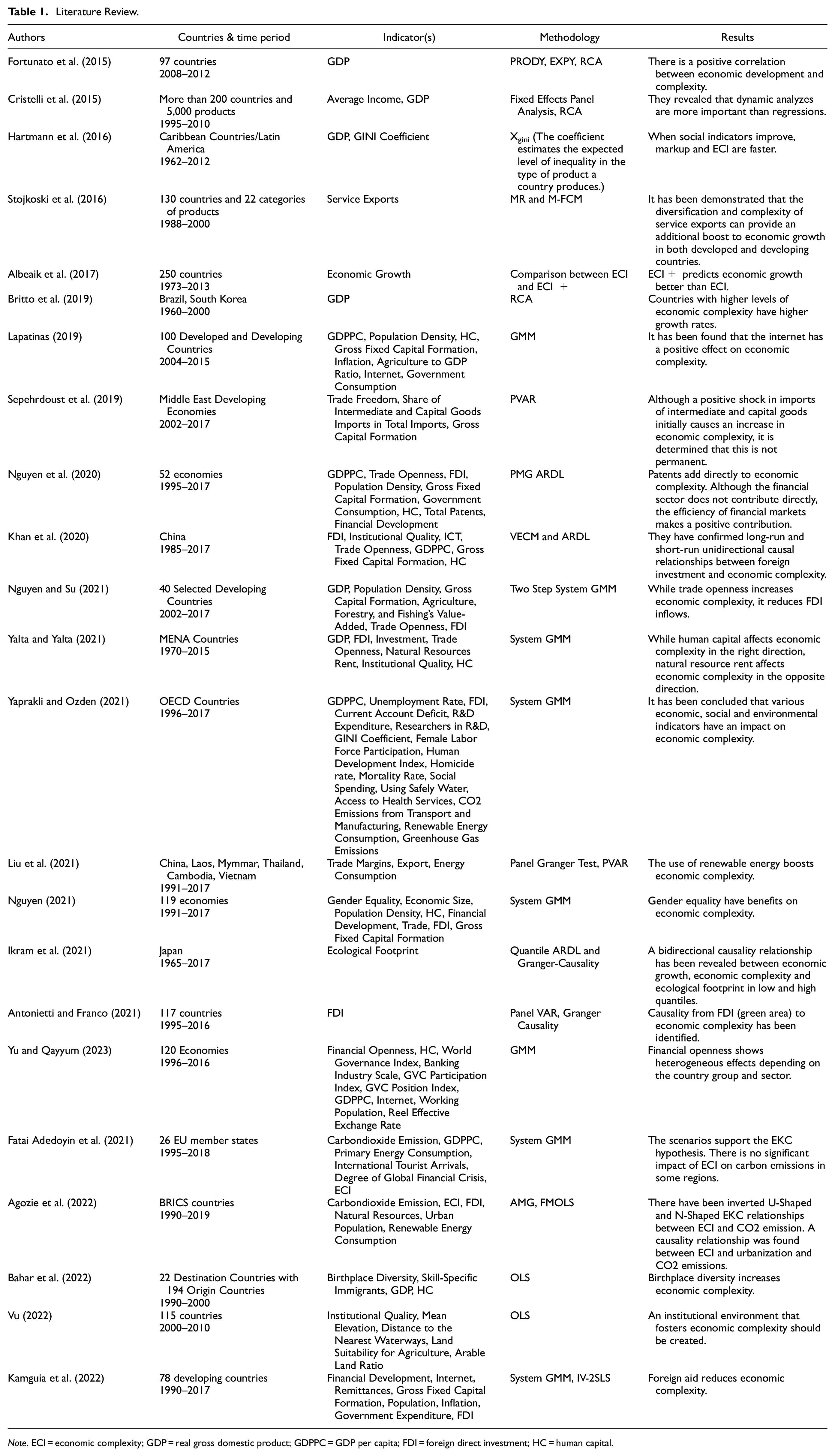
Note. ECI = economic complexity; GDP = real gross domestic product; GDPPC = GDP per capita; FDI = foreign direct investment; HC = human capital.

Methodology

The following approach was determined according to the literature given in Table 1 and extended from a different point of view. The study includes three methodologies: Index construction, capital stock estimation, and econometric analysis. First, we calculated five indexes from proxy variables as a comprehensive dataset. The independent variables of the model consist of these indexes. Thus, the number of variables was limited, and their scope was expanded. To calculate the indexes, we used a two-step method. First, we calculated dimensional indices. In this context, variables with different scales were normalized based on their minimum and maximum values between 0 and 1. The final index is the geometric mean of the dimension indices. ¹ The dimension indices are calculated as follows;

$$I_{\mathrm{ij}}=\frac{X_{\mathrm{ij}}^z-\underset{k}{min}\left\{X_{\mathrm{ik}}^z\right\}}{\underset{k}{max}\left\{X_{\mathrm{ik}}^z\right\}-\underset{k}{min}\left\{X_{\mathrm{ik}}^z\right\}}i=1,...,k\mathrm{ve}z=1,...,N$$

(1)

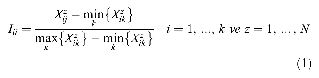
In the Equation 1, $I_{\mathrm{ij}}$ is the dimensional indice. $X_{\mathrm{ij}}$ is the related variable value for the unit $j$ , and at the time $i$ . $\underset{k}{min}\left\{X_{\mathrm{ik}}\right\}$ , and $\underset{k}{max}\left\{X_{\mathrm{ik}}\right\}$ define the minimum and maximum values of $X$ (Anand & Sen, 1993; UNDP, 2020). While $I_{\mathrm{ij}}^{X_N}$ is the dimension indice of the variable $X$ for the unit $j$ , and at the time $i$ , the final index $H_{\mathrm{ij}}$ is:

$$H_{\mathrm{ij}}=(I_{\mathrm{ij}}^{X_1}*...*I_{\mathrm{ij}}^{X_N}{)}^{1/N}$$

(2)

The published capital stock data set, which includes an up-to-date and systematic approach, is unavailable for countries. For this reason, capital stock estimates (CSE) are another step in the study. We utilized the perpetual inventory method (PIM), accumulating past gross investments by deducting their depreciated value (Nehru & Dhareshwar, 1993). The capital stock $K_t$ is constructed according to the:

$$K_t=(1-\phi {)}^{t}K(0)+\sum _{i=0}^{t-1}{I}_{t-i}(1-\phi {)}^i$$

(3)

The variables in Equation 3 consist of the initial capital stock $K(0)$ , investment $I_t$ , and depreciation rate $\phi$ . Gross fixed capital formation is the primary data for investment $I_t$ in literature. To estimate the initial capital stock, Equation 3 can be rewritten based on Harberger (1978) as follows:

$$K_{t-1}=I_t/(g+\delta )$$

(4)

where $g$ is the output growth rate, and $\delta$ is the depreciation rate.

The final stage of the analysis is estimating panel models for mapping out drivers of economic complexity. We decided on the econometric model with the diagnostic tests. Breusch and Pagan (1980) LM test and Hausman test were used to determine which of the Panel FE (Panel Fixed Effects), Panel RE (Panel Random Effects), and Pooled OLS models were appropriate for hypothetical tests. We tested heteroscedasticity in regression residuals with the modified Wald test, considering the fixed effects model. Meanwhile, the relationship between error terms for successive time intervals was checked with Wooldridge (2002) and Drukker (2003) autocorrelation tests. The cross-sectional dependence, which is the autocorrelation between the panel units, was examined by the Pesaran (2004) CD test. Lastly, we tested the stationarity with Pesaran (2003) CADF by considering the cross-sectional dependence. As a result of diagnostic tests, it has been determined that Ordinary Least Squares (OLS) assumptions are not fulfilled. Since the assumptions of ordinary least square are considered to be violated, the 2SGMM system is preferred in the study. For robustness check, the same method is used by considering the three-year averages of the variables (Appendix 2). The use of averages of the variables will benefit us as we will be able to minimize the impact of business cycles on the data set. Due to the nature of the data in this study, we employ a two-step generalized method of moments (2SGMM) model. The GMM technique is suitable for panel data sets with cross-sections (N) larger than the number of periods (t). GMM is a robust estimation methodology in the presence of endogeneity, serial correlation and heteroskedasticity problems (Arellano & Bond, 1991, 1998; Arellano & Bover, 1995; Baum et al., 2003; Blundell & Bond, 1998). ²

In the empirical literature on the estimation of linear dynamic panel data models with a large number of cross sections (N) and a relatively small number of periods (T), generalized method of moments (GMM) estimators are widely used. GMM methods traditionally assume that disturbances are cross-sectionally independent. The GMM method is not robust under cross-section dependence; however, CSD weakens when T<N (Sarafidis et al., 2009). Ullah et al. (2018) suggest using GMM estimators to better control for the three sources of endogeneity (unobservable heterogeneity, simultaneity and dynamic heterogeneity).

For these reasons, the two-step system GMM estimator is an optimized solution to provide efficient and consistent forecasts in the panel data set and avoid the problems mentioned.

Data Set and Model

The data set used in the research contains 97 countries and the period of 1995 to 2020. Economic Complexity Index (ECI) is the dependent variable in the model. Control variables are determined by following the studies in the literature (Table 1). Moreover, the choice of variables is ultimately based on the theoretical framework of the Neoclassical School and Endogenous Growth Models. We calculated five indexes from interrelated variables to increase their inclusiveness and representativeness. Thus, the model’s independent variables are the Education Index (EI), Institutional Quality Index (IOI), Health Index (HI), Macroeconomic Situation Index (MSI), Openness Index (OI), and Capital Output Ratio (COR). Table 2 shows the indexes and related sub-indices.

Table 2.

Description of the Data Set.

Variable	Unit	Description	Data sources
ECI	Index	Economic Complexity Index	Harvard Growth Lab
EI	Index	Education Index	Author’s calculation
ce	Years	Compulsory education duration	World Bank (2023)
se	Years	Secondary education duration	World Bank (2023)
ays	Years	Average years of total schooling	Barro and Lee (2013)
eg	%	Ratio of government education expenditure to government expenditure	World Bank (2023)
ey	%	Ratio of government education expenditure to GDP	World Bank (2023)
IQI	Index	Institutional Quality Index	Author’s calculation
cc	Score	Control of corruption	World Bank (2023)
ge	Score	Government effectiveness	World Bank (2023)
ps	Score	Political stability and absence of violence/terrorism	World Bank (2023)
rq	Score	Regulatory quality	World Bank (2023)
rol	Score	Rule of law	World Bank (2023)
va	Score	Voice and accountability	World Bank (2023)
HI	Index	Health Index	Author’s calculation
hb	Number	Hospital beds-per 1,000 people	World Bank (2023)
le	Years	Life expectancy at birth	World Bank (2023)
md	%	Lifetime risk of maternal death	World Bank (2023)
mor	%	Mortality from CVD, cancer, diabetes or CRD between exact ages 30 and 70	World Bank (2023)
MSI	Index	Macroeconomic Situation Index	Author’s calculation
er	%	Employment to population ratio-15+	World Bank (2023)
y	USD	GDP per capita-at constant 2015	World Bank (2023)
$\pi$	%	Inflation, consumer prices-annual	World Bank (2023)
lpr	%	Labor participation rate-15+	World Bank (2023)
OI	Index	Openness Index	Author’s calculation
fdi	%	Foreign direct investment, net inflows (of GDP)	World Bank (2023)
op	%	Openness	World Bank (2023)
ex	%	Exports of goods and services (of GDP)	World Bank (2023)
imp	%	Imports of goods and services (of GDP)	World Bank (2023)
KY	Index	Capital Output Ratio (K/Y)	Author’s calculation
ı	USD	Gross fixed capital formation (constant 2015)	World Bank (2023)
K	USD	Capital stock	Author’s calculation
Y	USD	GDP-at constant 2015	World Bank (2023)

ECI refers to the productive knowledge base of the country. The products produced in the country are the measure of the knowledge of the society. The main components of ECI calculations are the variety of exports a country produces and the number of countries capable of producing them. Thus, following Hidalgo and Hausmann (2009), the mix of the variety of export products and the prevalence of countries producing them is used as a proxy variable to indicate the capabilities available in the country and required for a product. The greater the number and complexity of a country’s exported products, the higher the ECI value. We obtained the ECI dataset, which covers the period 1995 to 2020, from the Harvard Growth Lab. Therefore, the analysis of the study also includes the same countries and periods. Meanwhile, the ECI was normalized to harmonize with the independent variables that are used as indexes in the model.

The EI consists of the duration of education, the length of secondary education, the average years of total education, the ratio of government spending on education to total government spending, and the ratio of government spending on education to GDP. All variables included in the EI affect the index in the same direction. The IQI index consists of six variables: Anti-Corruption, Government Effectiveness, Political Stability and Absence of Violence/Terrorism, Regulatory Quality, Rule of Law, and Voice and Accountability. These variables indicate the current perceptions of the country’s citizens on specific issues. Control of corruption refers to the perception of the extent to which public power is abused for personal gain. Government effectiveness shows the quality of public services, the extent to which they are free from political pressure, and confidence in the government to implement policies. Regulatory quality symbolizes the principles and rules of government that enable and encourage private sector development. The rule of law encompasses the quality of society’s rules, property rights, trust in the police and courts, and the degree of compliance. Finally, voice and accountability include citizens’ participation in electing their government, freedom of expression, freedom of association, and free media. Again, all variables in the IQI index have the same direction of influence in terms of institutional quality. HI contains four sub-indices. While hospital beds per person and life expectancy at birth have a positive effect on the index, the lifetime risk of maternal death and mortality from cancer, diabetes, etc. have a negative effect. Therefore, we included the inverse value of the last two variables in the sub-dimensions indices. Similarly, the MSI consists of the employment rate, GDP per capita, labor force participation rate, and the inverse of the inflation rate. Since inflation moves in the opposite direction compared to other variables in terms of economic stability, it was used as ${\pi }^{-1}$ . Thus, the direction of influence of all variables in the index has been made the same. We used foreign direct investment and openness as proxy variables for openness (OI). Finally, the model includes the capital-output ratio (KY) as a control variable. We also normalized this variable to ensure its harmony with the other variables.

We developed the model to examine the drivers of economic complexity. The closed and open forms of the model are, respectively:

$$\mathrm{ECI}=f\{\mathrm{EI},\mathrm{IQI},\mathrm{HI},\mathrm{MSI},\mathrm{OI},\mathrm{KY}\}$$

(5)

$$\begin{array}{c}\multicolumn{1}{c}{\mathrm{ECI}={\beta }_0+{\beta }_{1}E{I}_{\mathrm{it}}+{\beta }_2\mathrm{IQ}{I}_{\mathrm{it}}+{\beta }_{3}H{I}_{\mathrm{it}}+{\beta }_4\mathrm{MS}{I}_{\mathrm{it}}}\\ \multicolumn{1}{c}{+{\beta }_{5}O{I}_{\mathrm{it}}+{\beta }_{6}K{Y}_{\mathrm{it}}+{\epsilon }_{\mathrm{it}}}\end{array}$$

(6)

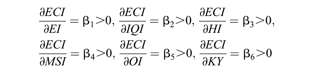
Additionally, the indexes are defined as follows;

$$\mathrm{EI}=f\{\mathrm{ce},\mathrm{se},\mathrm{ays},\mathrm{eg},\mathrm{ey}\}$$

(7)

$$\mathrm{IQI}=f\{\mathrm{cc},\mathrm{ge},\mathrm{ps},\mathrm{rq},\mathrm{rol},\mathrm{va}\}$$

(8)

$$\mathrm{HI}=f\{\mathrm{hb},\mathrm{le},\mathrm{md},\mathrm{mor}\}$$

(9)

$$\mathrm{MSI}=f\{\mathrm{er},y,\pi ,\mathrm{lpr}\}$$

(10)

$$\mathrm{OI}=f\{\mathrm{fdi},\mathrm{op}\}$$

(11)

All parameters estimated in the model will be expected to be positive values:

$$\begin{array}{c}\multicolumn{1}{c}{\frac{\partial \mathrm{ECI}}{\partial \mathrm{EI}}={\beta }_1>0,\frac{\partial \mathrm{ECI}}{\partial \mathrm{IQI}}={\beta }_2>0,\frac{\partial \mathrm{ECI}}{\partial \mathrm{HI}}={\beta }_3>0,}\\ \multicolumn{1}{c}{\frac{\partial \mathrm{ECI}}{\partial \mathrm{MSI}}={\beta }_4>0,\frac{\partial \mathrm{ECI}}{\partial \mathrm{OI}}={\beta }_5>0,\frac{\partial \mathrm{ECI}}{\partial \mathrm{KY}}={\beta }_6>0}\end{array}$$

(11)

Empirical Findings

With economic development, productive knowledge and its use in industry are also promoted. In this way, countries begin to produce more and more sophisticated products. Therefore, ECI is also a critical proxy variable for economic development. Table 3 shows the ECI ranking, that is, the variety and complexity of the countries’ exported products for the top 20 and the bottom 20 countries.

Table 3.

ECI Ranking: The Top 20 and the Last 20 Countries (2020).

Rank	Country	ECI	Change over 10 years	Rank	Country	ECI	Change over 10 years
1	Japan	2.265	0	114	Malawi	−0.962	0
2	Switzerland	2.140	0	115	Botswana	−0.963	−34
3	Germany	1.961	0	116	Mozambique	−0.976	11
4	South Korea	1.949	4	117	Ghana	−1.024	−14
5	Singapore	1.872	−1	118	Mali	−1.025	−25
6	Czechia	1.780	1	119	Ecuador	−1.097	−19
7	Austria	1.696	−2	120	Cuba	−1.162	−32
8	Sweden	1.593	−2	121	Azerbaijan	−1.242	0
9	Hungary	1.542	1	122	D. R. of Congo	−1.268	4
10	United Kingdom	1.540	1	123	Mauritania	−1.271	10
11	Slovenia	1.540	3	124	Côte d’Ivoire	−1.351	−7
12	USA	1.473	0	125	Venezuela	−1.374	−2
13	Slovakia	1.430	2	126	Papua New Guinea	−1.474	4
14	Finland	1.402	−5	127	Cameroon	−1.619	−9
15	Ireland	1.348	2	128	R. of Congo	−1.641	0
16	Italy	1.335	0	129	Nigeria	−1.734	3
17	China	1.300	7	130	Gabon	−1.833	−10
18	France	1.288	−5	131	Guinea	−1.911	0
19	Romania	1.274	9	132	Liberia	−2.238	−28
20	Mexico	1.216	−2	133	Angola	−2.506	−4

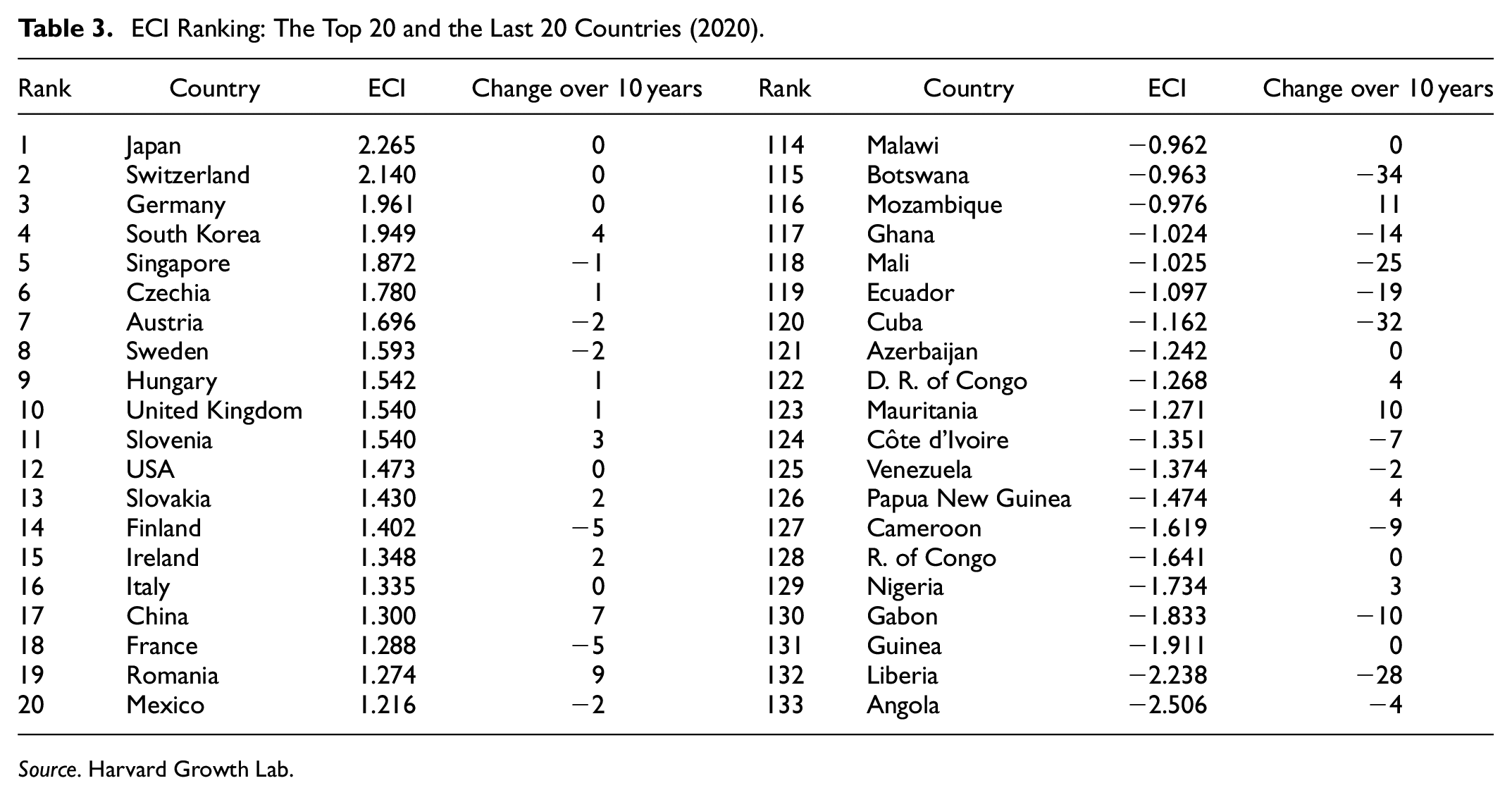
Source. Harvard Growth Lab.

Countries with more complex export products rank higher in Table 3, while those with less complex ones rank lower. Japan has the highest ECI score of 133 countries, and its rank has not changed over 10 years. Switzerland and Germany, ranked second and third, respectively, are countries whose rankings have remained the same over the past decade. Romania and China are the countries whose rankings have improved the most among the top 20. The countries ranked in the last 20 are at the bottom of the panel in terms of per capita income level (Appendix 1). Meanwhile, ECI rankings for 1995 and 2020 are mapped comparatively in Figure 1.

Figure 1.

Country complexity ranking: 1995 to 2020.

If the ECI exceeds the level of sophistication allowed by the country’s income, this situation probably indicates faster future growth. Therefore, these countries are also in an advantageous position for the future. One should remember this point when interpreting Table 3 and Figure 1. Descriptive statistics are reported in Table 4. The variable with the highest coefficient of variation (cv) is HI, and the lowest is EI. So, the educational index has a more homogeneous distribution around the arithmetic mean among all variables. In terms of the health index, there is a more heterogeneous situation.

Table 4.

Descriptive statistics.

Variables	N	Mean	SD	Variance	Cv	Min	Max
ECI	3,433	0.496	0.176	0.031	0.355	0.002	1.000
EI	3,021	0.475	0.139	0.019	0.292	0.049	0.868
IQI	3,591	0.503	0.223	0.050	0.444	0.003	1.000
HI	3,562	0.157	0.121	0.015	0.770	0.002	0.610
MSI	3,456	0.347	0.158	0.025	0.456	0.011	0.917
OI	3,218	0.145	0.050	0.003	0.348	0.002	0.486
KY	2,984	0.234	0.119	0.014	0.507	0.002	1.000

Note. N = number of observations; SD = standard deviation; cv = coefficient of variation (SD/mean).

We have examined the pairwise correlations that show the relationships between the binary variables and provide insight into the issues that can be explored through extended analysis. Table 5 shows the correlation matrix with the significance level of the correlation between the variables. According to the a priori results, there is a positive and statistically significant linear correlation between the pairs of variables. The variables that have the highest correlation with ECI are HI and IQI. The most correlated variables are HI-IQI and IQI-MSI.

Table 5.

Pairwise Correlations.

Variables	ECI	EI	HI	IQI	KY	MSI	OI
ECI	1.000
EI	.475***	1.000
	(.000)
HI	.787***	.572***	1.000
	(.000)	(.000)
IQI	.743***	.407***	.755***	1.000
	(.000)	(.000)	(.000)
KY	.244***	.150***	.248***	.147***	1.000
	(.000)	(.000)	(.000)	(.000)
MSI	.554***	.304***	.656***	.753***	.128***	1.000
	(.000)	(.000)	(.000)	(.000)	(.000)
OI	.206***	.039**	.205***	.242***	.129***	.219***	1.000
	(.000)	(.044)	(.000)	(.000)	(.000)	(.000)

Note.***p < .01. **p < .05. *p < .1.

We examined heteroscedasticity, autocorrelation and cross-sectional dependence in the regression residuals. The modified Wald test statistic shows that the variance of error terms is not constant (Table 6). That is, the residual of regression has heteroscedasticity. According to Wooldridge (2002) test results, we rejected the null hypothesis, stating that there is no autocorrelation (Table 6). This result shows that the error terms are sequentially related.

Table 6.

Heteroskedasticity and autocorrelation.

Test	Test type	Test statistics	p-Value
Heteroskedasticity	Modified Wald Test	9,488.26	.000
Autocorrelation	Wooldridge F Test	34.915	.000

Note. The null hypothesis of the wald test (H₀): No heteroscedasticity (homoscedasticity). The null hypothesis of the F test (H₀): No autocorrelation.

We tested the cross-sectional dependence with Pesaran’s (2004) CD test and rejected the null hypothesis. Hence, panels have a cross-sectional dependence for the residual and the variables (Table 7). That is, the individual units are interrelated and not independent.

Table 7.

Cross-sectional Dependence.

Variables	CD-Test	p-Value	Correlation	Absolute correlation	Number of groups
ECI	−1.530	.126	−.003	.412	133
EI	255.360	.000	.624	.773	112
HI	357.100	.000	.739	.778	132
IQI	2.620	.009	.005	.429	133
MSI	149.950	.000	.320	.550	128
OI	81.259	.000	.170	.360	118
KY	84.830	.000	.206	.517	117
Residual	2.790	.005	.009	.418	97

Note. Under the null hypothesis of cross-section independence CD ~ N(0,1).

It is necessary to test the stationarity by considering the cross-sectional dependence. For this reason, we examined the stationarity of the variables with Pesaran’s (2003) CADF test and presented the test statistics in Table 6. The null hypothesis, which shows the series is not stationary, has not been rejected. Since regression analysis assumes that the associated time series is stationary, it involving non-stationary time series causes nonsense regression. However, the series becomes stationary at the first difference. To avoid alleviating the data, we used the series as a level. However, we checked whether there is a nonsense regression phenomenon through a cointegration test and a unit root test on regression residuals in our model.

If the variables that are integrated in the same order are also cointegrated, we can trust the regression analysis results. Table 8 shows that all variables are integrated of order one-I(1). We also analyzed whether the series are cointegrated with Westerlund’s (2005) cointegration test by considering the cross-sectional dependence (Table 9). According to the test result, the null hypothesis, meaning the series are not cointegrated, has been rejected. Therefore, the variables move together in the long run, and the regression results will also be reliable.

Table 8.

CADF Unit Root Test.

Variables	Level			First difference
	t-bar	Z[t-bar]	p-Value	t-bar	Z[t-bar]	p-Value
ECI		−0.598	.275		−8.000	.000***
EI		1.619	.947		−2.650	.004***
HI		4.769	1.000		−9.605	.000***
IQI	−2.288	0.394	.653	2.772	−5.606	.000***
MSI	1.525	9.667	1.000	−2.870	−6.693	.000***
OI		1.218	.112		2.821	.002***
KY		5.247	1.000		−9.732	.000***

Note. The null hypothesis (H₀) assumes that all series are not stationary. ***Indicates that the null hypothesis was rejected at the 1% significance degree. Constant term + trend critical values: 10%: −2.490, 5%: −2.540, 1%: −2.630. Because the panel is unbalanced, only the standardized Z-Bar statistic can be calculated in some series.

Table 9.

Cointegration Test.

Test type	Test statistics	p-Value
Variance ratio	4.6558	.0000

Note. Null hypothesis (H0): Series are not cointegrated. Cross-sectional means removed.

The problems of heteroscedasticity, autocorrelation and cross-sectional dependence have different potential effects on the regression analysis. We applied the dynamic 2SGMM method and robust standard errors for heteroscedasticity to minimize the serial correlation between these possible effects. In two-step estimation, the standard covariance matrix is already robust in autocorrelation and heteroscedasticity theoretically. Dynamic regression findings are presented in Table 10.

Table 10.

Two-step System GMM Coefficients by Income Level.

Variables	(1)	(2)	(3)	(4)
	Panel overall	High income	Middle income	Low income
L.ECI	.371***	.687***	.360***	.203***
	(.007)	(.023)	(.048)	(.054)
EI	.062***	.069***	−.143***	−.335**
	(.009)	(.015)	(.051)	(.164)
HI	.387***	.122***	.777***	1.128***
	(.014)	(.035)	(.144)	(.423)
IQI	.100***	.033*	.114***	.336***
	(.009)	(.020)	(.036)	(.112)
KY	.051***	.216***	−.049	.0160
	(.007)	(.017)	(.032)	(.103)
MSI	.134***	.025	.108**	−.525**
	(.015)	(.022)	(.042)	(.248)
OI	.066***	.158***	.198*	1.07***
	(.012)	(.043)	(.102)	(.172)
t	−.002***	−.001***	−.0008***	.0014**
	(9.30e-05)	(.0002)	(.0003)	(.0007)
Constant	.105***	.034**	.191***	.213**
	(.009)	(.016)	(.029)	(.097)
Observations	2,332	986	759	587
Number of id	97	40	32	25
Number of i.v	80	32	31	28
Wald chi2	8,279.57	8,553.16	931.65	470.67
[prob.]	[.000]	[.000]	[.000]	[.000]
Arellano-Bond AR(1)	−5.00	−3.76	−2.90	−3.03
[prob.]	[.000]	[.000]	[.004]	[.002]
Arellano-Bond AR(2)	1.34	0.60	1.17	−0.43
[prob.]	[.179]	[.547]	[.243]	[.669]
Sargan Test	26.09	22.28	24.56	14.65
[prob.]	[1.000]	[.504]	[.319]	[.744]
Hansen Test	81.00	32.40	19.44	18.87
[prob.]	[.195]	[.092]	[.618]	[.465]

Note. Standard errors in parentheses. Probability values in brackets. ***p < .01, **p < .05, *p < .1. Hansen and Sargan test H0: The instruments are valid. t is time trend. We used Windmeijer (2005) finite-sample correction for the two-step covariance matrix.

It can be seen from the data in Table 10 that Wald statistics show that the models are significant. In all models, the lagged dependent variable (L.ECI) was specified as endogenous, while all other control variables were treated exogenously to reduce the number of instrumental variables. The validity of the instrumental variables was tested by the Sargan and Hansen test. Since the p-value of the test statistic is more significant than 5%, the validity of the instrumental variable is confirmed. Therefore, the choice of instrumental variables in the models is reasonable. Moreover, the test statistics reported for AR(1) indicate a high first-order correlation in each model, while AR(2) does not show a second-order correlation. These test statistics indicate an appropriate specification for the two-stage system GMM. Diagnostic tests imply that the 2SGMM estimation is robust and that the standard errors are unbiased. Therefore, the estimated coefficients and statistics are reliable.

Firstly, the lagged variable (L.ECI) indicates a positive and significant association with economic complexity in all income levels. Thus, a one-point rise in lagged ECI results in a 0.37-point increase in complexity. That implies that a rise in previous ECI would heighten the current sophisticated production in economies.

The coefficient of EI is positive for the panel overall and for the high-income group but significant and negative for the middle and low-income groups. Across the panel, when the education index increases by one-point, economic complexity increases by approximately 0.06 points. In high-income countries, the size of the coefficient is more prominent. Therefore, among high-income countries, those with higher values of this variable tend to export more diverse and complex products and have more productive know-how. We consider that the negative effect of this variable on education in middle-income and low-income countries is related to the quality of education in these countries. Moreover, the labor force with human capital may not be able to contribute sufficiently to economic complexity in these countries as a result of being mis-matched with the incorrect jobs. The HI variable has a positive coefficient in all groups and across the panel. Besides, it is the variable with the highest impact on the panel overall. The impact capacity of the variable increases toward lower income. This shows that in low-income countries, human capital affects economic complexity through health rather than education. When the health index increases by one point, it positively affects economic complexity by approximately 0.39 points. Therefore, countries with higher variable values in all country groups tend to export more diverse and complex products. Improvements in countries’ health indicators also favor productive know-how. We suggest that the high health effect at low-income levels is due to the progress in human capital related to health rather than education in these countries. IQI positively and significantly affects ECI for all income groups. A one-point increase in the institutional quality index increases the economic complexity index value by 0.10 points. However, the effect of the coefficient tends to increase toward the lower-income group. IQI is the variable with the highest influence in the lower-income group. That is due to the relative institutional quality gap between lower-income and high-income groups. Therefore, countries where corruption is under control and political stability, accountability, the rule of law and institutional quality are adopted are advantageous in terms of productive know-how. Moreover, they have a higher potential to export more diverse and complex products. MSI is positive and statistically significant for both middle-income and panel overall. A positive one-point increase in the macroeconomic stability index stimulates economic complexity by 0.13 points in the same direction. Therefore, countries with high labor force participation, employment rates and per capita income have an advantage in terms of the diversity and complexity of export products. Moreover, the magnitude of the coefficient is relatively high for the panel. This finding suggests that price stability also favors economic complexity.

KY is positively and significantly associated with ECI in both panel overall and high-income countries. A positive one-point increase in the capital stock index stimulates economic complexity by 0.05 points and 0.22 points in the same direction, panel and high-income countries, respectively. Therefore, as the capital structure strengthens in high-income countries, the tendency to export more diverse and complex products and to have more productive knowledge increases. Although the variable has a negative coefficient in middle-income and low-income countries, it is statistically insignificant. We assess that the results obtained for those countries are related to the quality and allocation efficiency of the capital stock in those countries. If the allocation efficiency is not ensured, the physical capital increase may not support growth and exports. The analysis’ expansion by considering the allocation efficiency and quality of the physical capital stock will be a key study subject. OI, which consists of FDI and openness to internationalization, statistically significantly and strongly affect the diversity and complexity of export products in all groups. However, openness to externalization stimulates complexity more as we move toward lower-income groups. This leads to the conclusion that openness in low-income groups, which suffer from a lack of capital accumulation, contributes significantly to complexity. Therefore, a one percentage point increase in OI leads to a 0.07 percentage point increase in ECI across the panel. However, the magnitude of the variable jumps to 1.07 in the low-income group. This result suggests that trade and FDI encourage sophisticated production through spillover effects.

Conclusion and Policy Recommendation

The provision of sustainable growth and prosperity depends on the conditions that will enable them. Considering economic complexity and product range dynamics allows us to expose the links between economic development and growth precisely. This study set out to analyze the drivers of economic complexity by adopting a dynamic panel data methodology on low-middle-upper income countries for the years 1995 and 2020.

Using multivariate 2SGMM regression, we checked for measures of economic complexity for health, education, macroeconomic stability, institutional quality, and openness for the past 25 years. Moreover, we also examined this relationship by income groups in countries. Panel-overall findings indicate that all explanatory variables are positive and statistically significant. In the high-income group, the primary determinant of economic complexity is openness and capital stock. The health components and institutional quality power the economic complexity in low-income and institutional quality and macroeconomic stability in the middle-income groups. It is also found that openness to foreign trade significantly impacts middle and high-income groups. Our results illustrate that the complexity of an economy, therefore, a country’s potentially sophisticated products, is strongly linked with institutional quality, the health dimension of human development, openness and macroeconomic stability. However, the effect magnitudes of education and capital stock are relatively limited across the panel. They indicate that the significant complexity dynamics differ according to country groups. Firstly, entire health policies that will increase life expectancy at birth and well-functioning institutional structures will stimulate economic complexity. Institutional quality is essential to support long-term development and economic complexity, especially for low- and middle-income countries. Only by boosting institutional quality will the structural transformation process in the economy accelerate. As emphasized in the studies of Hausmann and Rodrik (2003) and Hidalgo and Hausmann (2009), increasing welfare in the future is possible with this transformation. At this point, Gani and Prasad (2006) examined the export structure of six Pacific Island countries over four essential indicators of institutional quality (control of corruption, rule of law, government effectiveness and regulatory quality). They revealed that improvements in institutional quality variables are important for general trade and improved exports. Similarly, Ebi and Eke (2018) emphasized that economic diversity can be achieved by strengthening the indicators of corruption control, political stability, rule of law and government effectiveness. Nganga (2021), as in the studies of Ebi and Eke (2018), stated that corruption control would contribute to economic diversification in the long run. Vu (2022) also supports our empirical inferences. Vu (2022) found that even variables such as rule of law, corruption control, and state effectiveness represent good institutions. The establishment of stable political systems is crucial in improving economic diversity. However, it is essential to adopt good governance the rules to avoid favoritism that may hinder the country’s development. Cervantes and Villaseñor (2015) emphasized in their study that the fight against corruption, which is pursued together with governance, will significantly impact the economy. There is a consensus in the economic literature that trade openness and FDI inflows are important for technology and economic development (Ghebrihiwet, 2019). Our findings on both variables are consistent with the existing literature and support Nguyen’s (2021) results.

Although the education dimension of human capital is significant only in the high-income group and across the panel, its effect is weak. The insignificant impact on education in middle-income and low-income countries is related to the quality of education in these countries. This finding is consistent with the literature suggesting that export-led growth will be achieved through an increase in human capital increase. Policies that focus only on increasing the duration of education will need to be revised, especially in low-income groups. At the same time, conditions that will improve the quality of education should also be provided.

Gross fixed capital is another determinant of productive capacity. It creates the necessary conditions for the production of diversified and high-tech products. Sepehrdoust et al. (2019) and Nguyen (2021) found that gross fixed capital formation positively affects economic complexity. These studies support our empirical findings in terms of their results. The present results are also important for some policy implications respects. Economies, particularly middle- and low-income ones, must transform or improve their institutional structures to include precise, clear, objective rules to boost the capability of producing sophisticated products. The policy sets that promote democracy, the rule of law, and property rights will also foster economic complexity. The findings might further indicate that economies should keep policies contributing to healthy life years on the agenda for sustainable growth. Considering the impact of CVD, cancer, diabetes or CRD diseases on mortality risk and labor productivity, health policies supporting preventive health services and early diagnosis are seen as another area for improvement. Meanwhile, investigating the sensitivity of economic complexity to different factors affecting healthy life years is another topic for future research. The study also has policy implications in the area of education. The production technology required by sophisticated products necessitates the existence of a labor force capable of using this technology. The education policies of economies should support the training of human resources that can ensure technological developments and keep pace with these developments. Countries should reinforce informal education processes such as on-the-job training and formal education to strengthen professional skills and competencies. The impact of vocational programs that increase the quality of the labor force on economic complexity awaits future researchers as another study topic.

Consequently, this study offers important implications for explaining the determinants of economic complexity in terms of income groups. Policymakers should ensure increased economic complexity by executing the economy in the right direction. Considering the importance of countries producing knowledge and skill-intensive products and diversifying their export structures for sustainable growth, the implications of this study are also noteworthy.

As with any empirical analysis, the study’s limitations are directly proportional to the data quality and the model efficiency. To minimize these limitations, we have restricted the period to a specific year and analyzed countries in subgroups that are homogeneous in income level. We are subject to this restriction because ECI data were unavailable before 1995. Moreover, we check the coefficients for robustness to ensure consistency.