Sage Journals: Discover world-class research

Abstract

The purpose of this study is to investigate people’s image of income distribution and its difference by social position from data collected during a 2015 Japanese survey (SSP 2015) by applying Bayesian statistical analytical models. The income distribution image denotes the perceived and estimated income distribution of the individual and is supposed to be a basis of subjective belief on the features of society, including societal average income. In this study, the latent income distribution images were estimated from the observed variable of average income image. Furthermore, differences in income distribution image by social position were analyzed using Bayesian hierarchical models. The differences in income distribution image by age cohort and household income class were examined in terms of the mean (expected value) and the Gini inequality coefficient of the distribution image. It was found that although the distribution image tends to underestimate the average income level and overestimate inequality, the income distribution image could be an incomplete reflection of the income distribution characteristics of the reference group.

Keywords

income distribution social cognition inequality reference group Bayesian hierarchical model

In the field of sociology, many scholars have focused on cognition of social aspects and phenomena, as well as the formation of beliefs or society image, as a basis of rational actions or choices of actors. This is especially true in cognitive sociology (Zerubavel, 1997) and in analytical sociological theories such as the DBO (desire-belief-opportunity) theory (Hedström, 2005), or in the cognitivist model for rational choice (Boudon, 1996, 1998).

Among these social cognitive features, I will focus on people’s image of income distribution in this study. The income distribution image denotes the perceived and estimated income distribution by the individual and is supposed to be formed by the understanding of own income status and others’ income status and a basis of subjective belief on the features of society, including societal average income. This income distribution image is important for policy making, as it represents the people’s assessment of the state of inequality in society, and consequently, forms a basis of people’s choice of redistribution policies and regimes (Cruces, Perez-Truglia, & Tetaz, 2013).

Several attempts have been made to capture income distribution image. Among them, Norton and Ariely (2011) directly examined Americans’ image of the distribution of wealth in the United States, as well as their preference for ideal distribution through an online survey. The authors clearly showed that respondents’ wealth distribution image shows greater equality than the actual distribution.

In line with Norton and Ariely (2011), Cruces et al. (2013) further examine the biased perception of income distribution. In particular, they examine how individuals form biased perceptions of their own relative position in income distribution and how these perceptions affect redistribution preferences. From a household survey in Argentina, they found that there are systematic biases in individuals’ evaluations of their relative position in income distribution, which can be partly explained by the extrapolation of information from endogenous reference groups.

Related to the studies directly exploring perception of income distribution, there are series of studies exploring the perception of legitimacy or inequality of income distribution (i.e., Amiel & Cowell, 1999; Caricati, 2017; Cowell & Cruces, 2004).

I examine current Japanese income distribution image in this study, not directly from the respondents’ estimated income distribution per se, like Norton and Ariely (2011), but indirectly from respondents’ estimated average income collected by a nationwide random sampling interview survey. I will employ a Bayesian statistical model to analyze people’s image of income distribution from average income image data.

Recently, Bayesian statistics and its application have been developed in many fields, and there have been an increasing number of applications in the field of social sciences, including sociology (Jeliazkov & Yang, 2014; Western, 1999, 2001). This “Bayesian renaissance” is mainly attributable to the recent remarkable development of computational Markov chain Monte Carlo (MCMC) methods that enable us to bypass mathematical derivation of posterior distributions, which can be hard to solve.

The virtues of Bayesian statistics vis-à-vis conventional frequentist statistics can be summarized as follows: (a) the natural assumption of an inference process that resembles a human inference process—it is assumed that a prior belief, represented as a prior parameter distribution, meets some empirical data and turns out to be a more concrete posterior belief, represented as a posterior distribution; (b) flexible model construction that enables us to express multilevel uncertainty with hierarchical models; and (c) the possibility of connection to formal theoretical models of a Bayesian learning process of formation of belief. Based on these virtues, I would like to insist that Bayesian statistics is more suitable for social psychological studies of image of distribution than frequentist statistics, because it enables us to construct flexible models that express uncertainty of image by parameter distribution, and it allows for investigation of image formation mechanisms behind the image distribution as Bayesian inference or learning process (Breen, 1999; Breen & García-Peñalosa, 2002).

Thus, this study aims to investigate people’s image of income distribution and its difference by social position using observed data from a 2015 Japanese survey, by applying Bayesian statistical analytical models. The remainder of this article is structured as follows: first, the method is discussed in terms of data and variables. Thereafter, three different Bayesian models for examining income distribution image are discussed. For each model, the assumptions are outlined and the results are discussed. Finally, the conclusion provides perspective to the results and outlines future work.

Method

Data

The data used for the analysis are from the Stratification and Social Psychology Project Survey (SSP 2015),¹ which is a Japanese national sampling survey of class identity, social images, and other related attitudes toward social inequality and social stratification. The survey was conducted between January and June 2015. The sampling procedure was a three-stage stratified random sampling, and the sampling list was the Japanese electoral roll and the basic resident registration. Questionnaires were distributed to 8,309 male and female participants aged 20 to 64 years in 450 locations, and the mode of data collection was face-to-face interviews with computer (tablet-type device) assistance (Computer Assisted Personal Interview [CAPI]). Consequently, there were 3,573 valid responses. The survey was conducted with the respondents’ informed consent, and anonymity was retained throughout the survey process. The official response rate was 43.03%.²

Variables

The variable of income distribution image per se is not available in the SSP 2015 data. Instead, the variable of average income image is available, that is, a respondent’s estimation of the average income of the same generation as the respondent. The actual question for average income image is “how much do you think the average annual income of people your age is?” Then, respondents were asked to select a corresponding income class as the answer.³ In the following analysis, I treat the average income image variable as a continuous variable using the median value of the income class.

It can be assumed that the average income image is derived from the latent and unobserved income distribution image of the individual. I will analyze the variation of income distribution image and its differentiations from observed average income image by applying Bayesian hierarchical models. Theoretically, the difference in income distribution image by social position may result from the differences in respondents’ social experience and social interaction with others by their social position.

Figure 1 shows the distribution of average income image.⁴ The median is 425 ten thousand Japanese yen, the mean is 437 ten thousand Japanese yen, and the standard deviation is 215.

Figure 1.

Histogram of average income image (ten thousand Japanese yen).

Model 1: Overall Shared Income Distribution Image

Model Definition

First, I introduce a simple prototype model with assumption of overall shared income distribution image. I assume that each respondent’s average income image (which is directly observed in the survey) derives from a sample mean of the respondents’ latent and unobserved income distribution image. The latter is assumed to be shaped by a lognormal distribution represented by $\log N (μ, σ)$ , where parameters μ and σ are the mean and standard deviation of the variable’s natural logarithm. Especially for Model 1, I assume that all respondents share a latent income distribution image.

The reasons for assuming a lognormal distribution as the income distribution image are as follows. First, it has been theoretically and empirically claimed that the actual income distribution closely approximates the lognormal distribution, especially when excluding the higher income group (Clementi & Gallegati, 2005; Gibrat, 1931; Hamada, 2004; Pestieau & Possen, 1979; Sargan, 1957). Second, the lognormal distribution is easy to handle parametrically for obtaining the indices of the features of distribution, such as the mean (expected value) and the Gini coefficient. Although the actual income distribution image may have various forms beyond the parametric assumption, I employ the assumption of lognormal distribution as the first approximation.

For simplicity of the model, let us assume that people properly estimate the societal average income from unbiased information of their income distribution image.⁵ If each value $Y_{1}, Y_{2}, \dots, Y_{n}$ was sampled IID (i.e., independent and identically distributed) from the distribution image $\log N (μ, σ)$ , then respondent i’s observed average income image ${\bar{Y}}_{i}$ derived from the mean of the sampled values would be asymptotically normally distributed, according to the central limit theorem. That is,

\begin{array}{l} {\bar{Y}}_{i} = n^{- 1} \sum_{k = 1}^{n} Y_{k}, \\ Y_{k} ~_{i i d} \log N (μ, σ) \end{array}

{\bar{Y}}_{i} ~_{a s y m} N (m, s / \sqrt{n})

where m and s are the mean (expected value) and standard deviation of shared latent income distribution image, obtained by the following equations:

m = \exp {μ + σ^{2} / 2},

s = \sqrt{\exp {2 μ + σ^{2}} (\exp {σ^{2}} - 1)} .

For the sake of simplicity in the MCMC simulation, it is also assumed that the sample size n is constant—concretely, n = 100—which means that the average income image is obtained by aggregating the income information of 100 persons.

With reference to the method of setting of prior distributions by Kruschke (2015), I assume that μ is normally distributed as $N (\hat{μ}, 10^{2} \hat{σ})$ , and σ is uniformly distributed from $\hat{σ} / 10^{3}$ to $10^{3} \hat{σ}$ , where $\hat{μ}$ and $\hat{σ}$ are point estimations of μ and σ from actual data.⁶ These assumptions of prior distributions are set for being less informative and noncommittal prior distributions.

Figure 2 is the graphical representation of Model 1, where gray circle nodes indicate observed continuous variables (image of average income in this model), double circle nodes indicate generative continuous variables (parameters of normal distribution of average income image), single circle nodes indicate latent continuous variables with prior distribution (parameters of shared latent income distribution image with the shape of lognormal distribution), and square nodes indicate latent discrete variables (assumed sample size from latent income distribution image). Figure 3 shows the outline of Model 1.

Figure 2.

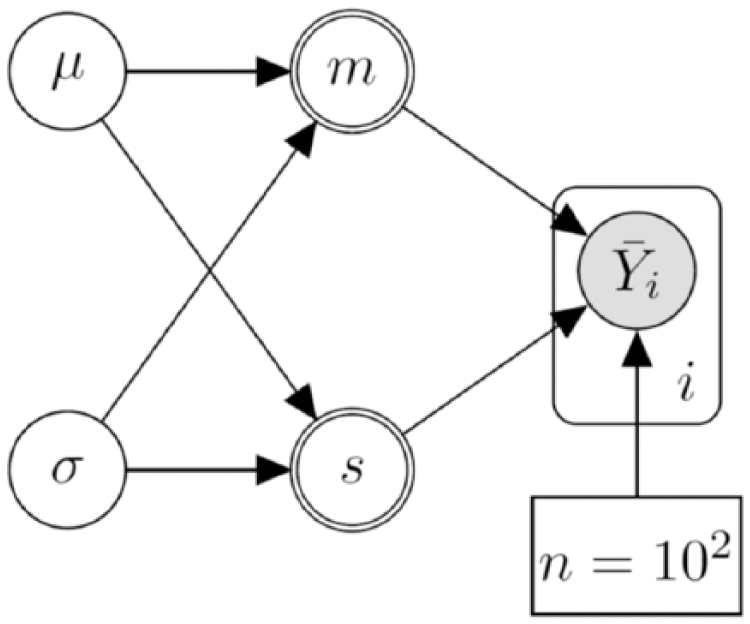
Graphical model of Model 1.

Figure 3.

Outline of Model 1.

Result of the MCMC Estimation

I employed Stan 2.13.1 (Stan Development Team, 2016b) for the MCMC simulation programming to estimate the posterior distributions of parameters μ and σ, and RStan 2.13.2 (Stan Development Team, 2016a) for implementation in R. I conducted four chains of sampling for 5,000 iterations each, which includes 1,000 initial iterations as burn-in samples. The thin interval was set as one, to generate 16,000 sampled points of posterior distribution.

Table 1 shows the summary of the MCMC estimation of posterior distributions for Model 1. Gelman–Rubin MCMC convergence statistic ( $\hat{R}$ ) of each parameter is around 1.000; hence, we can safely conclude that the MCMC sampling converged (Gelman et al., 2013). The means of posterior distribution of μ and σ, which are parameters of a lognormally shaped income distribution image, are 4.467 ([4.427, 4.505] as 95% credible interval) and 1.797 ([1.782, 1.812]), respectively, and the means of m and $s / \sqrt{n}$ , which are parameters of normal distribution of observed average income image, are 437.427 ([430.171, 444.604]) and 215.359 ([210.348, 220.523]), respectively. For any of the parameters, the credible intervals are sufficiently small, indicating that the estimation results are sufficiently stable and convincing.

Table 1.

Summary of MCMC Estimation (Model 1).

Parameter	M	SE	SD	2.50%	25%	50%	75%	97.50%	ESS	$\hat{R}$
µ	4.466	0.000	0.020	4.425	4.453	4.466	4.480	4.506	3,030.58	1.001
σ	1.797	0.000	0.008	1.781	1.792	1.797	1.802	1.813	3,065.35	1.001
m	437.319	0.055	3.754	429.945	434.795	437.346	439.849	444.642	4,722.92	1.000
$s / \sqrt{n}$	215.374	0.036	2.616	210.232	213.602	215.322	217.094	220.626	5,196.00	1.001
G	0.796	0.000	0.002	0.792	0.795	0.796	0.797	0.800	3,065.10	1.001

Note. MCMC = Markov chain Monte Carlo; ESS = effective sample size; $\hat{R}$ = Gelman–Rubin MCMC convergence statistic.

I monitored the Gini coefficient of income distribution image as a transformed parameter. The Gini coefficient of the lognormal income distribution is parametrically obtained by the following formula (Aitchison & Brown, 1957).

G = 2 Φ (\frac{σ}{\sqrt{2}}) - 1,

where $Φ$ is the cumulative distribution function of the standard normal distribution. The mean of G is 0.796 ([0.792, 0.800]), which is a considerably high rate in reality.

Figure 4 shows the shared income distribution image predicted by the posterior distributions of the parameters of the lognormal distribution; it comprises an overlay of 100 plots whose parameters were randomly resampled from the MCMC sample. Figure 5 comprises the histogram of the observed average income image, overlaid by randomly resampled 100 posterior predictive distributions.

Figure 4.

Predicted shared income distribution image (ten thousand Japanese yen).

Figure 5.

Data with posterior predictive distribution (ten thousand Japanese yen).

Let us compare the estimated shared income distribution image with the actual household income distribution in Japan at that time. According to the Comprehensive Survey (CSLC) of Living Conditions 2015,⁷ the actual average household income in 2015 is 541.9 ten thousand Japanese yen, and the value of the Gini coefficient is 0.401.⁸ The estimated shared income distribution image tends to underestimate wealth (average income) and highly overestimate inequality (the Gini coefficient) in the society.

Model 2: Difference of Shared Income Distribution Image Among Age Cohorts

Model Definition

Although Model 1 is a relatively simple prototype model in which all respondents hold the same image of income distribution, it can be theoretically assumed that people hold different images, based on their different social experiences. Based on sociological theories of reference groups (e.g., Hyman, 1942; Merton, 1957), it can be assumed that people form their image of income distribution mainly by integrating information on incomes of their reference group members with whom they interact daily. Thus, the image is an incomplete reflection of the income distribution of the reference group. The latter is assumed to be selected based on either geographic proximity or similarity in terms of attributes and socioeconomic status (Singer, 1981). Hence, images can differ with social position.

As the scope of reference is clearly set on age in the actual question of average income image in this survey, the age cohort is the first to be considered as a category that causes differences in the income distribution image. In the actual analysis, I created a nominal variable of age cohort, consisting of categories of 10-year duration between 20 and 59 years of age, such as 20s (aged 20-29 years) and 30s (aged 30-39 years), and the 60s category from 60 to 64 years old. Furthermore, samples were divided by gender because typical features of an age cohort within the reference group could differ by gender, especially in Japan, where gender roles and rules still strongly constrain their life courses (Kano, 2015).

In the analytical model, the difference of shared income distribution image among each category is described as the difference in parameters of the latent income lognormal distribution, μ and σ. Besides, I assume that the parameter μ is predicted by a linear equation, that each parameter of the equation has its distributions, and that the parameter σ obeys a gamma distribution. This model resembles the ANOVA model in frequentist statistics (Kruschke, 2015). However, it is more flexible, as we can estimate not only differences of $μ$ m but also differences of σ, with no strict assumptions.

The average income image held by the ith individual in the jth category, denoted by ${\bar{Y}}_{i j}$ , is assumed to be determined by

\begin{array}{l} {\bar{Y}}_{i j} = n^{- 1} \sum_{k = 1}^{n} Y_{k j}, \\ Y_{k j} ~_{i i d} \log N (μ_{j}, σ_{j}) \end{array}

and its distribution is

{\bar{Y}}_{i j} ~_{a s y m} N (m_{j}, s_{j} / \sqrt{n}),

\begin{array}{l} m_{j} = \exp {μ_{j} + σ_{j}^{2} / 2}, \\ s_{j} = \sqrt{\exp {2 μ_{j} + σ_{j}^{2}} (\exp {σ_{j}^{2}} - 1)} . \end{array}

The parameter $μ_{j}$ is predicted by the following equation

μ_{j} = β_{0} + \sum_{j} β_{j} x_{j} (i) .

(1)

In Equation 1, $x_{j} (i)$ represents an index function in which an individual i that falls in category j of the nominal predictor is represented by $x_{j} (i) = 1$ ; if not, then $x_{j} (i) = 0$ . It is assumed that each $β_{j}$ obeys an identical normal distribution $N (0, σ_{β})$ , and that the sum of $β_{j}$ is 0. Meanwhile, the parameter $σ_{j}$ is assumed to obey a gamma distribution

σ_{j} ~ g a m m a (M o_{σ_{j}}, S d_{σ_{j}})

where $M o_{σ_{j}}, S d_{σ_{j}}$ represent the mode and standard deviation of the distribution, respectively. Finally, prior distributions of parameters or hyperparameters of the model are defined as follows, in line with Kruschke (2015)⁹:

β_{0} ~ N (\hat{μ}, 10 \hat{σ}),

σ_{β} ~ g a m m a (\frac{\hat{σ}}{2}, 2 \hat{σ}),

M o_{σ_{j}} ~ g a m m a (\frac{\hat{σ}}{2}, 2 \hat{σ}),

S d_{σ_{j}} ~ g a m m a (\frac{\hat{σ}}{2}, 2 \hat{σ}) .

Figure 6 comprises the graphical representation of Model 2, and Figure 7 represents its outline.

Figure 6.

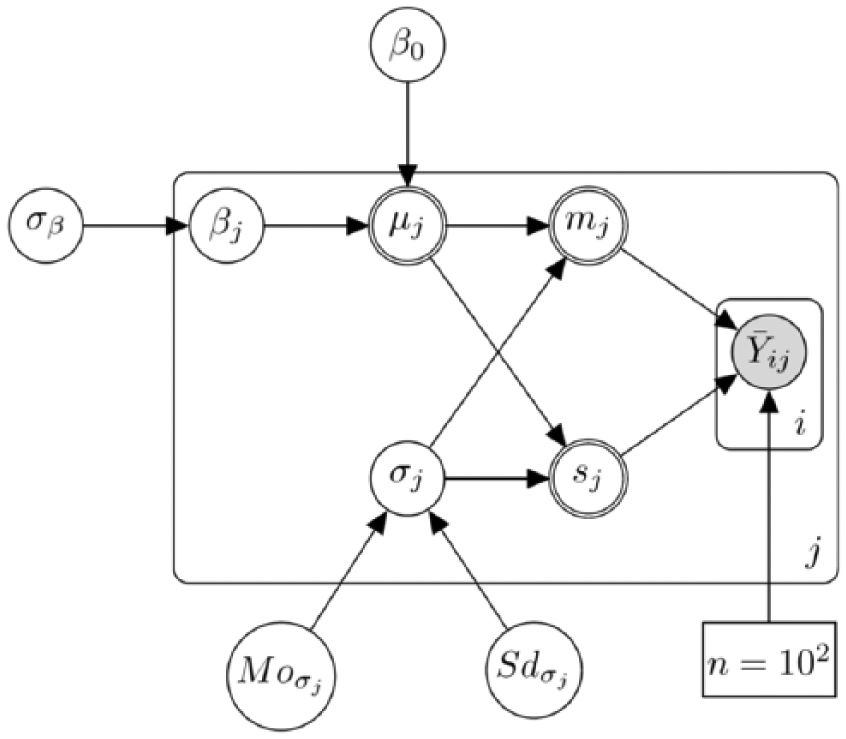
Graphical model of Model 2.

Figure 7.

Outline of Model 2.

Results of the MCMC Estimation

As for Model 2, I also conducted four chains of sampling for each of the 5,000 iterations, which includes 1,000 initial iterations as burn-in samples. Thereafter, the thin interval was set as one, generating 16,000 samples of the posterior distribution.

As for the male sample, $\hat{R}$ of each estimated parameter is lower than 1.02; therefore, the MCMC sampling converged. Table 2 shows posterior distributions of parameters determining different income distribution images for different categories.

Table 2.

Summary of MCMC Estimation (Model 2, Male Sample).

Parameter	M	SE	SD	2.50%	25%	50%	75%	97.50%	ESS	$\hat{R}$
$β_{0}$	4.565	0.000	0.030	4.506	4.545	4.566	4.586	4.622	14,568.51	1.000
$β_{20 s}$	−0.562	0.001	0.076	−0.721	−0.612	−0.560	−0.510	−0.420	13,263.37	1.000
$β_{30 s}$	−0.012	0.000	0.053	−0.116	−0.048	−0.012	0.024	0.090	15,573.46	1.000
$β_{40 s}$	0.289	0.000	0.047	0.195	0.257	0.289	0.322	0.381	13,257.54	1.000
$β_{50 s}$	0.460	0.000	0.048	0.366	0.428	0.461	0.492	0.553	14,087.80	1.000
$β_{60 s}$	−0.175	0.001	0.063	−0.302	−0.217	−0.174	−0.132	−0.056	14,289.09	1.000
$σ_{20 s}$	1.857	0.000	0.033	1.794	1.834	1.856	1.879	1.923	13,256.24	1.000
$σ_{30 s}$	1.723	0.000	0.024	1.676	1.707	1.723	1.740	1.772	15,269.29	1.000
$σ_{40 s}$	1.636	0.000	0.023	1.593	1.621	1.636	1.651	1.681	13,256.19	1.000
$σ_{50 s}$	1.617	0.000	0.023	1.573	1.601	1.616	1.632	1.661	15,186.22	1.000
$σ_{60 s}$	1.795	0.000	0.028	1.741	1.776	1.795	1.814	1.851	13,971.90	1.000

Note. MCMC = Markov chain Monte Carlo; ESS = effective sample size; $\hat{R}$ = Gelman–Rubin MCMC convergence statistic.

Model 2 with the female sample can also be regarded as being converged. Table 3 shows posterior distributions of the parameters determining different income distribution images for categories.

Table 3.

Summary of MCMC Estimation (Model 2, Female Sample).

Parameter	M	SE	SD	2.50%	25%	50%	75%	97.50%	ESS	$\hat{R}$
$β_{0}$	4.315	0.000	0.031	4.254	4.294	4.316	4.336	4.375	16,000.00	1.000
$β_{20 s}$	−0.444	0.001	0.073	−0.592	−0.493	−0.443	−0.394	−0.307	16,000.00	1.000
$β_{30 s}$	0.121	0.000	0.054	0.013	0.084	0.121	0.157	0.225	16,000.00	1.000
$β_{40 s}$	0.372	0.000	0.050	0.274	0.339	0.373	0.406	0.468	16,000.00	1.000
$β_{50 s}$	0.321	0.000	0.053	0.216	0.286	0.321	0.356	0.422	16,000.00	1.000
$β_{60 s}$	−0.369	0.001	0.070	−0.514	−0.415	−0.367	−0.321	−0.236	16,000.00	1.000
$σ_{20 s}$	1.909	0.000	0.029	1.853	1.888	1.908	1.928	1.967	16,000.00	1.000
$σ_{30 s}$	1.747	0.000	0.024	1.701	1.730	1.747	1.763	1.794	16,000.00	1.000
$σ_{40 s}$	1.725	0.000	0.021	1.684	1.711	1.725	1.739	1.767	16,000.00	1.000
$σ_{50 s}$	1.784	0.000	0.022	1.743	1.769	1.784	1.799	1.829	16,000.00	1.000
$σ_{60 s}$	1.932	0.000	0.028	1.879	1.913	1.932	1.950	1.988	16,000.00	1.000

Note. MCMC = Markov chain Monte Carlo; ESS = effective sample size; $\hat{R}$ = Gelman–Rubin MCMC convergence statistic.

The differences of the means and the Gini coefficients of lognormally shaped income distribution images in age cohorts are shown in Figures 8 and 9, respectively. For both male and female samples, the mean of the distribution image increases as the age cohort rises until the 50s and then decreases in the 60s. As for the Gini coefficient, although the values are relatively high, there is a U-shape tendency in which the 50s (for the male sample) or the 40s (for the female sample) have the lowest unequal image.

Figure 8.

Mean of shared income distribution image (median and 95% credible interval).

Figure 9.

Gini coefficient of shared income distribution image (median and 95% credible interval).

Finally, I compared the estimated shared income distribution image of each age cohort with the actual household income distribution of the age cohort. Table 4 shows the actual average household income and the Gini coefficient of each age cohort in 2015 from CSLC 2015 and the SSP 2015 data. Each estimated shared income distribution image tends to underestimate wealth (average income) and overestimate inequality (the Gini coefficient) in the society; still, these images approximately reflect tendencies in difference among age cohorts.¹⁰

Table 4.

Actual Average Household Income and the Gini Coefficient in Age Cohort.

Surveys	20s(below 29 years in CSLC 2015)	30s	40s	50s	60s
CSLC 2015Average income	365.3	558.9	686.9	768.1	525.8
SSP 2015Average income	591.84	600.35	690.92	785.37	585.57
SSP 2015Gini coefficient	0.385	0.309	0.308	0.363	0.431

Note. CSLC = Comprehensive Survey of Living Conditions; SSP = Stratification and Social Psychology.

Model 3: Difference of Shared Income Distribution Image Among Income Classes

We can apply another categorical variable or a set of categorical variables to this Bayesian hierarchical model. Here is another model with an actual household income class that consists of four income categories divided by quartile points. Categories are below 375 ten thousand yen (c1), from 375 to 600 (c2), from 600 to 800 (c3), and above 800 (c4). The structure of the model and the procedure of MCMC sampling are same as Model 2 (see Figures 6 and 7).

Table 5 shows the result of the estimation of posterior distributions of parameters determining different income distribution images for income classes, and Figures 10 and 11 show differences in the means and the Gini coefficients of lognormally shaped income distribution images in income classes. There is an explicit linear relationship between the mean of shared income distribution image and income class, that is, the mean of income distribution image increases significantly as the income class increases. On the contrary, the Gini coefficient of income distribution image decreases slightly as the income class increases. An explanation of such trends of the mean may be directly derived from reference group theory, which states that people tend to form their image by comparisons with others close to their social economic status (Merton, 1957). The trend of the Gini coefficient may be related to the narrowness of the reference scope in higher income classes.

Table 5.

Summary of MCMC Estimation (Model 3).

Parameter	M	SD	2.50%	25%	50%	75%	97.50%	ESS	$\hat{R}$
$β_{0}$	4.550	0.021	4.508	4.536	4.551	4.565	4.591	13,341.47	1.000
$β_{c 1}$	−0.544	0.042	−0.626	−0.572	−0.544	−0.515	−0.463	13,088.57	1.000
$β_{c 2}$	−0.051	0.035	−0.119	−0.074	−0.050	−0.027	0.018	14,714.01	1.000
$β_{c 3}$	0.251	0.037	0.177	0.226	0.251	0.276	0.322	14,335.74	1.000
$β_{c 4}$	0.343	0.032	0.280	0.322	0.343	0.366	0.405	13,411.75	1.000
$σ_{c 1}$	1.867	0.018	1.832	1.854	1.867	1.879	1.903	13,254.07	1.000
$σ_{c 2}$	1.719	0.017	1.686	1.707	1.718	1.730	1.752	14,097.20	1.000
$σ_{c 3}$	1.664	0.019	1.626	1.650	1.663	1.676	1.702	13,146.20	1.000
$σ_{c 4}$	1.693	0.015	1.664	1.683	1.693	1.703	1.724	12,820.36	1.000

Note. MCMC = Markov chain Monte Carlo; ESS = effective sample size; $\hat{R}$ = Gelman–Rubin MCMC convergence statistic.

Figure 10.

Mean of shared income distribution image (median and 95% credible interval).

Figure 11.

Gini coefficient of shared income distribution image (median and 95% credible interval).

Conclusion

Thus far, we have investigated people’s image of income distribution and its difference by social position from data collected during a 2015 Japanese survey, by applying Bayesian statistical analytical models.

The study concludes that the distribution image tends to underestimate the average income level and overestimate inequality.

The fact that people tends to underestimate the average income level implies a possibility that people tend to overlook the existence of higher income earners when imagining the income distribution of their reference group. If so, this study’s assumptions of lognormal distribution as the income distribution image and random sampling from the image should be reconsidered, and if necessary, revised in future studies. Besides, the assumption of lognormal distribution would be the main cause of overall increase in the values of the Gini coefficient.¹¹ Hence, the focus should only be on the relative differences among the values of the Gini coefficient in this study.

Despite the effects of the distributional assumption on the results of analyses, in general, the income distribution image could be seen as an incomplete reflection of the income distribution characteristics of the reference group.

I would like to highlight some implications for an actual redistribution policy. As a matter of principle, the opinion of people based on their subjective evaluations of current distributional situations should be respected in policy making and assessment. However, the result of this study implies that the image of income distribution varies according to the scope of the reference group. Besides, it implies that income distribution image would be biased by overlooking higher income earners. Therefore, these properties of income distribution image should be carefully considered in policy making.

Once again, I would like to stress several advantages of adopting the Bayesian model to study distribution image. First, we can make a strict assumption of latent image in the Bayesian hierarchical model. Second, we can extract some latent information through the flexible model. In this case, we extracted information about inequality of the distribution image in terms of the Gini coefficient.

Some future tasks remain, based on limitations of this study. First, the assumption of lognormal distribution as latent income distribution image should be reconsidered as per the lessons of this study. Second, as the models are relatively simplistic, future studies should develop more empirically realistic and complex models to explore causal mechanisms in the formation of societal images. Third, the Bayesian model of images presented in this article should be verified by direct observation of the images. Finally, a connection should be made to formal theoretical models for a comprehensive study of image and social cognition.

Footnotes

Appendix

Full Detail of the Questions for Average Income Image and Household Income.

Average income image	How much do you think the average annual income of people your age is? Please choose one of the following.
Household income	What was the total income of your household (all people living together as a family unit), before taxes, for the past year? Please include all casual income and extra income such as annual pension, dividends on stock shares, etc. (Please choose single answer)
1	None
2	Less than ¥250,000
3	¥250,000 or higher but less than ¥500,000
4	¥500,000 or higher but less than ¥750,000
5	¥750,000 or higher but less than ¥1,000,000
6	¥1,000,000 or higher but less than ¥1,250,000
7	¥1,250,000 or higher but less than ¥1,500,000
8	¥1,500,000 or higher but less than ¥2,000,000
9	¥2,000,000 or higher but less than ¥2,500,000
10	¥2,500,000 or higher but less than ¥3,000,000
11	¥3,000,000 or higher but less than ¥3,500,000
12	¥3,500,000 or higher but less than ¥4,000,000
13	¥4,000,000 or higher but less than ¥4,500,000
14	Approximately ¥5,000,000 (¥4,500,000 or higher but less than ¥5,500,000)
15	Approximately ¥6,000,000 (¥5,500,000 or higher but less than ¥6,500,000)
16	Approximately ¥7,000,000 (¥6,500,000 or higher but less than ¥7,500,000)
17	Approximately ¥8,000,000 (¥7,500,000 or higher but less than ¥8,500,000)
18	Approximately ¥9,000,000 (¥8,500,000 or higher but less than ¥9,500,000)
19	Approximately ¥10,000,000 (¥9,500,000 or higher but less than ¥10,500,000)
20	Approximately ¥11,000,000 (¥10,500,000 or higher but less than ¥11,500,000)
21	Approximately ¥12,000,000 (¥11,500,000 or higher but less than ¥12,500,000)
22	Approximately ¥13,000,000 (¥12,500,000 or higher but less than ¥13,500,000)
23	Approximately ¥14,000,000 (¥13,500,000 or higher but less than ¥14,500,000)
24	Approximately ¥15,000,000 (¥14,500,000 or higher but less than ¥15,500,000)
25	Approximately ¥16,000,000 (¥15,500,000 or higher but less than ¥16,500,000)
26	Approximately ¥17,000,000 (¥16,500,000 or higher but less than ¥17,500,000)
27	Approximately ¥18,000,000 (¥17,500,000 or higher but less than ¥18,500,000)
28	Approximately ¥19,000,000 (¥18,500,000 or higher but less than ¥19,500,000)
29	Approximately ¥20,000,000 (¥19,500,000 or higher but less than ¥20,500,000)
30	¥20,500,000 or higher but less than ¥25,000,000
31	¥25,000,000 or higher but less than ¥30,000,000
32	¥30,000,000 or higher but less than ¥40,000,000
33	¥40,000,000 or higher but less than ¥50,000,000
34	¥50,000,000 or higher but less than ¥60,000,000
35	¥60,000,000 or higher but less than ¥70,000,000
36	¥70,000,000 or higher but less than ¥80,000,000
37	¥80,000,000 or higher but less than ¥90,000,000
38	¥90,000,000 or higher but less than ¥100,000,000
39	¥100,000,000 or higher

Acknowledgements

The author thanks the Stratification and Social Psychology (SSP) Project for the permission to use the SSP 2015 survey. The author also thanks the editor, Jinxian Wang, and two anonymous referees for their helpful comments that improved the article. I am also grateful for comments on the author’s study made by Toru Kikkawa, Hiroshi Hamada, Yoshimichi Sato, and Gianluca Manzo.

Author’s Note

Atsushi Ishida is now at Kwansei Gakuin University, Japan.

Declaration of Conflicting Interests

The author(s) declared no potential conflicts of interest with respect to the research, authorship, and/or publication of this article.

Funding

The author(s) disclosed receipt of the following financial support for the research, authorship, and/or publication of this article: JSPS KAKENHI Grant Numbers 16H02045, 15K13080.

Notes

ORCID iD

Atsushi ISHIDA

Author Biography

Atsushi Ishida is a former associate professor at the faculty of human sciences, Osaka University of Economics, Japan. He is currently a professor at school of sociology, Kwansei Gakuin University, Japan. He mainly engages in mathematical and quantitative sociology of various research subjects including inequality and stratification, relative deprivation, and national identity.

References

Aitchison

Brown

J. A. C.

(1957). The lognormal distribution. Cambridge, UK: Cambridge University Press.

Amiel

Cowell

(1999). Thinking about inequality: Personal judgment and income distributions. Cambridge, UK: Cambridge University Press.

Boudon

(1996). The “cognitivist model”: A generalized “rational-choice model.” Rationality and Society, 8, 123-150.

Boudon

(1998). Social mechanisms without black boxes. In Hedström

Swedberg

(Eds.), Social mechanisms: An analytical approach to social theory (pp. 172-203). Cambridge, UK: Cambridge University Press.

Breen

(1999). Beliefs, rational choice and Bayesian learning. Rationality and Society, 11, 463-479.

Breen

García-Peñalosa

(2002). Bayesian learning and gender segregation. Journal of Labor Economics, 20, 899-922.

Caricati

(2017). Testing the status-legitimacy hypothesis: A multilevel modeling approach to the perception of legitimacy in income distribution in 36 nations. The Journal of Social Psychology, 157, 532-540.

Clementi

Gallegati

(2005). Pareto’s law of income distribution: Evidence for Germany, the United Kingdom, and the United States. In Chatterjee

Yarlagadda

Chakrabarti

B. K.

(Eds.), Econophysics of wealth distributions (pp. 3-14). Milano, Italy: Springer.

Cowell

Cruces

(2004). Perceptions of inequality and risk. Research on Economic Inequality, 12, 99-132.

10.

Cruces

Perez-Truglia

Tetaz

(2013). Biased perceptions of income distribution and preferences for redistribution: Evidence from a survey experiment. Journal of Public Economics, 98, 100-112.

11.

Gelman

Carlin

J. B.

Stern

H. S.

Dunson

Vehtari

Rubin

D. B.

(2013). Bayesian data analysis (3rd ed.). Boca Raton, FL: Chapman & Hall/CRC Press.

12.

Gibrat

(1931). Les Inégalités Économiques [Economic Inequalities]. Paris, France: Sirey.

13.

Hamada

(2004). A generative model of income distribution 2: Inequality of the iterated investment game. The Journal of Mathematical Sociology, 28, 1-24.

14.

Hedström

(2005). Dissecting the social: On the principles of analytical sociology. Cambridge, UK: Cambridge University Press.

15.

Hyman

H. H.

(1942). The psychology of status. Archives of Psychology, 269, 5-91.

16.

Jeliazkov

Yang

(Eds.). (2014). Bayesian inference in the social science. Hoboken, NJ: John Wiley.

17.

Kano

(2015). The future of gender in Japan: Work/life balance and relations between the sexes. In Baldwin

Allison

(Eds.), Japan: The precarious future (pp. 87-109). New York: New York University Press.

18.

Kikkawa

(2016). Dai 1 Kai SSP Chousa no Tokuchou [Properties of SSP 2015 Survey]. In SSP Project Office (Ed.), 2015nen Kaisou to Shakai Ishiki Zenkoku Chousa (Dai 1 Kai SSP Chousa) Houkokusho [SSP 2015 Survey Report]. Retrieved from http://ssp.hus.osaka-u.ac.jp/pdf/SSP-2015.pdf

19.

Kruschke

J. K.

(2015). Doing Bayesian data analysis: A tutorial with R, JAGS, and Stan (2nd ed.). London, England: Academic Press.

20.

Merton

R. K.

(1957). Social theory and social structure (Rev. ed.). New York, NY: The Free Press.

21.

Norton

M. I.

Ariely

(2011). Building a better America—One wealth quintile at a time. Perspectives on Psychological Science, 6(1), 9-12.

22.

Pestieau

Possen

(1979). A model of wealth distribution. Econometrica, 47, 761-772.

23.

Sargan

(1957). The distribution of wealth. Econometrica, 25, 568-590.

24.

Singer

(1981). Reference groups and social evaluations. In Rosenberg

Turner

R. H.

(Eds.), Social psychology: Sociological perspectives (pp. 66-93). New York, NY: Basic Books.

25.

Stan Development Team. (2016a). RStan: The R interface to Stan R package (Version 2.13.2). Available from http://mc-stan.org

26.

Stan Development Team. (2016b). Stan modeling language users guide and reference manual (Version 2.13.1). Available from http://mc-stan.org

27.

Western

(1999). Bayesian analysis for sociologists: An introduction. Sociological Methods & Research, 28, 7-34.

28.

Western

(2001). Bayesian thinking about macrosociology. American Journal of Sociology, 107, 353-378.

29.

Zerubavel

(1997). Social mindscapes: An invitation to cognitive sociology. Cambridge, UK: Harvard University Press.

A Bayesian Analysis of Income Distribution Image

Abstract

Keywords

Method

Data

Variables

Model 1: Overall Shared Income Distribution Image

Model Definition

Result of the MCMC Estimation

Model 2: Difference of Shared Income Distribution Image Among Age Cohorts

Model Definition

Results of the MCMC Estimation

Model 3: Difference of Shared Income Distribution Image Among Income Classes

Conclusion

Footnotes

Appendix

Acknowledgements

Author’s Note

Declaration of Conflicting Interests

Funding

Notes

ORCID iD

Author Biography

References