Sage Journals: Discover world-class research

Abstract

This study examines the association between fiscal sustainability indicators and Egypt’s economic growth from 1980 to 2018. Fiscal sustainability refers to a government’s ability to generate sufficient revenue to cover its costs and debt obligations in the long run without excessive borrowing or money creation. Egypt’s economic growth has slowed, raising questions about fiscal sustainability. This study aimed to analyze the dynamic relationship between fiscal sustainability indicators (government revenue, expenditure, external debt) and economic growth in Egypt. The autoregressive distributed lag (ARDL) bounds testing approach and unrestricted error correction model were applied to annual data from 1980 to 2018. A dynamic link was found between fiscal sustainability indicators and economic growth. Government expenditure and external debt significantly impacted economic expansion in the long term, while government revenue did not. Fiscal sustainability, measured by growth in total government expenses, external debt obligations, and revenue, significantly influences Egypt’s economic growth. Prudent fiscal management is crucial for sustained economic development. Policymakers should focus on controlling government spending, limiting external debt, and improving revenue generation to promote long-term economic growth in Egypt. Fiscal sustainability must balance critical investments in public services. Carefully managing fiscal deficits is key to unleashing Egypt’s economic potential. This study provides valuable insights into the connection between fiscal policy and economic growth in Egypt, informing policymakers’ decisions.

Plain Language Summary

Economic development potential in Egypt

The research examines the relationship between long-term fiscal policy and economic growth. We used data from 1980 until 2018 to determine Egypt’s capacity to cover its spending. The slowdown of economic development is a major reason for this research. The development trend of a country is an important signal of its further potential of being sustainable. Added value is crucial for ensuring equitable behavior across generations. Multiplying debts instead will diminish the capacity of the next generation to benefit from the same conditions as the generation before. Policymakers should decide on the implementation of strategic goals for this to happen. Our results highlight a dynamic link between fiscal sustainability indicators and economic growth. In the long term, government expenditure and external debt significantly impact economic expansion. Government revenue has a different impact. Prudent fiscal management is crucial for sustained development. Policymakers should focus on controlling government spending, limiting external debt, and improving revenue generation to promote long-term economic growth in Egypt. Additionally, fiscal sustainability must balance critical investments in public services. Carefully managing fiscal deficits is key to unleashing Egypt’s economic potential.

Keywords

fiscal sustainability fiscal sustainability indicators economic growth ARDL bounds test

Introduction

Sustainable development is a global challenge that requires various solutions, such as renewable energy, fiscal policy, and environmental protection. Renewable energy can enhance economic growth, productivity, and competitiveness (S. Ali et al., 2022; M. Ali et al., 2023; Asif et al., 2022, 2023; Ayad et al., 2023; Zhang et al., 2023). Fiscal policy can also boost economic growth, but it faces different challenges and views in developing countries. For example, fiscal policy can positively and negatively affect current and future generations, depending on how revenue is raised and spent (Hussain et al., 2021). Moreover, developing countries have difficulties mobilizing domestic resources and adopting effective spending strategies due to low tax bases, institutional problems, and a lack of research on optimal fiscal stances. Furthermore, economists have no consensus on the relationship between fiscal policy and economic growth. Some follow the Keynesian view that government spending causes economic growth, while others follow the neoclassical view that government spending affects economic growth but not output levels (Algaeed, 2022; Nyasha & Odhiambo, 2019).

Fiscal sustainability is essential for developing countries to achieve sustainable development. It can help developing countries bridge the financing gap, reduce debt burdens, and mobilize resources for investment in public policy priorities and the Sustainable Development Goals (SDGs). Fiscal sustainability can also help developing countries cope with external shocks and maintain macroeconomic stability and inclusive long-term growth. Fiscal sustainability involves assessing fiscal vulnerabilities, risks, and debt sustainability. Additionally, fiscal policy can help improve sustainability by incentivizing forest conservation and ecosystem health, which is vital for climate stability and reducing the risk of zoonotic diseases. Therefore, fiscal policy is a core component of governmental interventions that can influence countries’ development path and growth rate.

The issue of fiscal sustainability and its implications for economic growth has received increasing attention from policymakers in developing countries. Evaluating budget deficits and public debts that facilitate suitable economic expansion to achieve development goals has become critical. Many developing countries have implemented public finance reforms, including reducing deficits, improving tax systems, and increasing transparency and accountability. Reforms also control current spending, restructure social welfare programs, and maintain sustainable external debt levels to stimulate economic growth (Cigu et al., 2020; Coman Nuţă et al., 2023; Moldovan et al., 2014; Nuţă et al., 2015; Nuţă & Nuţă, 2020; Zeeshan et al., 2022). Egypt implemented significant reforms, focusing on higher revenue through broader tax bases, improved collection, reduced exemptions, including informal sectors, and combating evasion, especially the shadow economy. Though reforms aimed to create jobs and improve lives, more was needed to ensure fiscal sustainability and economic growth. Studies analyze fiscal sustainability’s future challenges as deficit and debt levels exacerbate the financial burden on future generations due to excessive public spending (Coman Nuţă et al., 2023; Lobont et al., 2018; Moldovan et al., 2014; Zeeshan et al., 2022). Egypt’s economy, society, and politics significantly impacted its finances since 1980. After 2012, Saudi-Egypt and Qatar-Egypt relations strained, with Qatar providing aid. After 2013, Gulf countries provided $15 billion in aid. Aids aimed to create jobs and improve lives, but more was needed to ensure fiscal sustainability and economic growth.

The relationship between fiscal variables such as government spending, taxes, debt, and economic growth is an important research area in public finance and macroeconomics. While a substantial body of literature examines this linkage, the findings remain mixed and inconclusive.

Previous studies have explored the relationship between fiscal sustainability and economic growth in Egypt. However, most of these studies have focused on debt sustainability rather than other aspects of fiscal sustainability. For example, Fathy Abdelgany and Badr Al-deen (2023) found that the Egyptian government’s fiscal policy was restrictive and unsustainable, as it failed to adjust its primary balance in response to the rising public debt. On the other hand, Al Sayed et al. (2021) argued that the fiscal policy in Egypt was sustainable from 1990/1991 to 2017/2018, based on a cointegration analysis. Our paper aims to fill the literature gap by examining fiscal sustainability’s impact on economic growth in Egypt, using a comprehensive measure of fiscal sustainability. There is still a need to explore this relationship further and determine the specific contributions of spending, revenue, and external debt to economic growth. This study aims to fill this gap by evaluating the impact of fiscal sustainability on economic growth in Egypt from 1980 to 2018, focusing on spending, revenue, and external debt individually to determine each’s contribution to economic growth. The study aims to provide policymakers with a better understanding of the impact of fiscal sustainability on economic growth, both short- and long-term, and submit proposals to improve fiscal sustainability and economic growth. We compare our results with other studies in the field and tie them to relevant literature. Overall, this study provides early warnings to policymakers, allowing policy changes to achieve economic growth while considering their effects and supporting decisions to continue or change fiscal policy. By analyzing fiscal sustainability indicators and their contribution to economic growth in Egypt, our study highlights the importance of fiscal sustainability for achieving sustainable development goals.

The structure of the paper is as follows: Section 2 highlights the main findings in the literature regarding fiscal sustainability, and Sections 3 and 4 present the dataset and the methodology. The results of this study are outlined in Section 5; discussion and conclusions are shown in the last two sections.

Literature Review

Theoretical Overview

Fiscal sustainability is essential for local governments worldwide (Gao et al., 2021; López Subires et al., 2019; Rodríguez Bolívar et al., 2016). Fiscal sustainability is a term used to describe the capacity of a government to maintain its spending and revenue policies over the long term without compromising its financial stability, risking bankruptcy, or defaulting on its future financial obligations. The government should be able to generate enough revenue to meet its current and future expenses without relying excessively on borrowing or creating inflation. ~~Public or government fiscal sustainability is one of the terms used in fiscal policies, but there has yet to be an agreement on a specific definition~~. In its definition of fiscal sustainability, the International Monetary Fund (IMF) depends on stabilizing the public debt ratio to GDP at a certain level or setting a specific target percentage. In this context, the IMF considers a country’s fiscal policies sustainable if it maintains a stable public debt ratio to GDP. This ratio is often used as an indicator of the government’s ability to manage its debt and avoid becoming overly indebted. A stable debt-to-GDP ratio can signal that the government can balance its budget over the long term and avoid borrowing to meet its expenses (Akyüz, 2007).

Fiscal Sustainability Indicators

The Tax gap indicator is a measure that illustrates the difference between the tax rate required for fiscal sustainability and the current tax rate. It indicates how much the tax burden would need to increase to achieve stability in the public debt-to-GDP ratio. A negative value of this indicator implies that current taxes are inadequate to stabilize the debt-to-GDP ratio, given the current spending policies. The tax gap indicator provides insight into the additional tax burden required to maintain stability in the debt-to-GDP ratio, considering current and expected future spending policies (Chalk & Hemming, 2000).

The Public debt to GDP ratio indicator is a metric that provides a clear understanding of the economic and financial burden on the public budget. When the ratio of public debt to GDP increases, the debt burden grows, and the government’s ability to pay off the debt decreases. This ratio is considered an essential indicator of fiscal sustainability by the International City Management Association, as it measures the ability of the government to meet its financial obligations and deliver public services without imposing an undue burden on future generations. High debt levels can constrain local government’s ability to finance public services and infrastructure and increase the risk of default or financial distress. Thus, monitoring and managing the debt burden of local governments is a crucial aspect of maintaining fiscal sustainability (Kluza, 2016).

Over time, indebtedness becomes a significant problem that threatens to achieve fiscal sustainability and economic growth. This indicator is divided into two types of indicators:

Indicators of internal public debt refer to debt issued and held by domestic residents or entities. It is a significant funding source for government budget deficits and is a common economic phenomenon in many countries. Managing internal public debt is a priority of fiscal policy, and efforts are made to either reduce the burden of this debt on the public budget or stabilize it.

Indicators of external public debt: External public debt is issued and held by non-resident creditors. In theory, some economists believe that external debt can contribute to economic growth in a country, as it provides additional financial resources. However, this is only the case if the debt is used to fund successful investments. Numerous studies have found that high levels of external debt can negatively impact a country’s economic growth rate.

The primary deficit indicator measures the government’s budget deficit before accounting for interest payments on debt. It is calculated by subtracting government revenue from government spending, excluding interest payments. A positive primary deficit means government spending is higher than the revenue, which increases the debt level.

Factors Affecting Fiscal Sustainability

Revenues and public expenditures: Revenues have a positive relationship with fiscal sustainability. The higher the revenue growth rates, the higher the fiscal sustainability index. As for public expenditures, they have an inverse relationship with fiscal sustainability if the rates of public spending are higher than the growth of public revenues, which leads to an expectation of a rise in the possibility of the government losing its fiscal solvency and the inability to enjoy fiscal sustainability. In order to achieve fiscal sustainability, there must be consistency between the growth of revenues and public expenditures. Higher public spending growth than the revenue growth rate for an extended period leads to a growth in the state’s budget deficit, which leads to more borrowing to pay off the deficit and then to a rise in the growth of debt and a threat to fiscal sustainability.

Public debt is a financial tool that governments use to finance spending when revenues fall short. It can be used to cover operational and investment expenditures, and when public spending exceeds revenues, it increases the government’s indebtedness. An increase in government spending in the present period leads to a growth in public debt and will represent a future burden on the public finances. This burden is usually passed on to future generations. The public spending policies must be such that the government can continue servicing its debts and avoid bankruptcy, meaning the public debt is sustainable. Public debt sustainability means that the government can meet all its financial obligations toward servicing the current and future debt while maintaining the ability to continue servicing the debt and avoiding arrears without restricting economic growth. For public debt to be sustainable, specific indicators set by the 1992 Maastricht Agreement (Stability and Growth Pact) must be met; it stipulates that the ratio of public debt to GDP should not exceed 60%. The Maastricht Agreement established a framework for the public debt-to-GDP ratio to be used as an indicator of public debt sustainability; it’s widely used as a benchmark among international organizations to assess debt sustainability.

Economic growth: is associated with fiscal sustainability. The rise in economic growth leads to higher income levels and increasing tax revenues, which reduces the gap between revenues and expenditures and raises investment and consumption rates. This process reduces internal and external financial borrowing and achieves fiscal sustainability and vice versa in the case of a decline in economic growth rates (Ayumu, 2004).

Interest rate is an economic factor that directly affects fiscal sustainability. A high interest rate leads to a rise in debt service (interest), whether these debts are external or internal, meaning an increase in the financial burden in the field of debt service, which leads to a decrease in the capacity of debt service. The government has to pay its internal or external debts, which negatively affects fiscal sustainability (Kathomi et al., 2017). There are various ways to understand fiscal sustainability. One standard definition is that it refers to a sufficient fiscal foundation that allows the government to implement its policies, fulfill its obligations, including unexpected expenses, and maintain macroeconomic stability and fairness in fiscal management across generations. The traditional method for evaluating sustainability is the debt-to-GDP ratio. Some methods take into account the time factor and more complexity. The research of Domar (1944) has significantly contributed to the debt sustainability discourse. The accounting approach, rooted in Domar’s rule, posits that for debt to be sustainable, the economic growth rate must surpass the interest rate on sovereign debt.

Additionally, the primary balance should be either positive or 0. However, even if these conditions are met, this method allows for very high debt-to-GDP ratios. One more approach is the Intertemporal Budget Constraint (IBC) which offers a theoretical foundation for current research in the field. It allows for an empirical examination of the dynamic aspects of fiscal variables by combining economic theory with econometric analysis. The IBC model and its testable hypotheses can be derived as follows. The IBC approach is a theoretical framework that combines economic theory with econometric analysis to comprehend the dynamic relationship between government debt, budget balance, and economic growth. It postulates that over the long term, a state can keep a sustainable debt level only if its primary surpluses’ present value equals its debt’s present value. An empirical examination of this relationship can provide insight into the dynamic behavior of government debt and its impact on economic growth. According to Hakkio and Rush (1991), Quintos (1995), and Martin (2000), the budget constraint for each period necessitates that the government’s expenditure on goods and services and transfer payments ( $G E_{t}$ ) and payments on past debt (represented by $(1 + i_{t}) B_{t - 1}$ , where it is the real interest rate and $B_{t - 1}$ is the principal and interest liability) must equal the total of revenue ( $R_{t}$ ) and new debt ( $B_{t}$ ) issued in the current period. This can be expressed as:

G E_{t} + (1 + i_{t}) B_{t - 1} = R_{t} + B_{t}

By performing the mathematical operations of addition and subtraction $i B_{t - 1}$ , we get:

$E_{t} + (1 + i) B_{t - 1} = R_{t} + B_{t}$ where $E_{t} = G E_{t} + (i_{t} - i) B_{t - 1}$ . We can use the forward iteration of this equation to get: $B_{t - 1} = \sum_{j = 0}^{\infty} β^{j + 1} (R_{t + j} - E_{t + j}) + \lim_{j \to \infty} β^{j + 1} B_{t + j}$ where $β = 1 / (1 + i)$ . Manipulating this equation further gives $G E_{t} + i_{t} B_{t - 1} = R_{t} + \sum_{j = 0}^{\infty} β^{j - 1} (Δ R_{t + j} - Δ E_{t + j}) + \lim_{j \to \infty} β^{j + 1} B_{t + j} .$

The fundamental principle of fiscal sustainability in the IBC approach is to match the present market value of debt with the estimated discounted value of future primary surpluses. This is equivalent to the notion of “no Ponzi game,” which means that the government’s fiscal policy should not depend on borrowing to finance current spending by promising future surpluses. This requirement necessitates that the limit term in the equation is equal to zero. The variable G represents government spending on goods and services, transfer payments, and interest payments on the accumulated debt. This implies that over the long term, the government should aim to produce primary surpluses to counteract debt accumulation and guarantee its sustainability. $G_{t} = G E_{t} + i_{f} B_{t - 1}$ . In addition, if G and R (i.e., government expenditure, including interest and revenue) are non-stationary series that are integrated of order one, their first differences will be stationary, as they follow difference stationary processes. Incorporating these conditions into the above equation gives the modified equation:

(R_{t} = α_{1} + R_{t - 1} + ε_{1 t}); G_{t} = α_{2} + G_{t - 1} + ε_{2 t} a n d \underset{j \to \infty}{l i m} . β^{j 1} B_{t + i}

\begin{matrix} G_{t} = α + R_{t} + ε_{t} where α = \sum β^{j - 1} (α 1 - α 2) and ε_{t} \\ = β^{j - 1} (ε_{1 t} - α ε_{2 t}) \end{matrix}

This equation can be presented in a regression form for hypothesis testing:

R_{t} = a + b G_{t} + ε_{t}

The modified equation is an extension of the IBC (Intertemporal Budget Constraint) model, which is used to study the dynamic aspects of fiscal variables and determine government debt sustainability. The IBC model is based on the principle that the current market value of government debt should be balanced with the expected discounted value of future primary surpluses, which is the difference between government revenue and expenditure, excluding interest payments. This principle is recognized as the “no Ponzi game” condition, which requires the limit term in the modified equation equal to zero, signifying that the government is not relying on indefinitely issuing new debt to meet its obligations. The IBC model assumes that government revenue and expenditure are integrated of order (1). This allows for an empirical analysis of the dynamic relationships between fiscal variables by economic theory and econometric techniques. The IBC model helps evaluate the sustainability of government debt over time, as it considers the time value of money and the dynamic nature of fiscal variables. It can be used to test various hypotheses about the relationships between fiscal variables and make projections about the future trajectory of government debt. A vital aspect of the IBC model is the primary balance, which is the difference between government revenue and expenditure, excluding interest payments. A primary surplus means the government generates more revenue than its spending, while a primary deficit indicates the opposite. To achieve fiscal sustainability, it is generally necessary for the government to maintain a primary surplus or at least a balance of zero; this ensures that the government has the resources to meet its current and future obligations. Another important consideration is the debt-to-GDP ratio, which measures the size of the government’s debt relative to the size of the economy. A high debt-to-GDP ratio can be a concern. It may indicate that the government is relying heavily on borrowing to finance its operations and may struggle to meet its debt obligations. However, it is essential to note that the debt-to-GDP ratio should be considered in conjunction with other factors, such as the government’s primary balance and the economic growth rate, as these can also affect the sustainability of government debt.

Furthermore, it is essential to note that the IBC model is a theoretical framework. Its assumptions and results should be carefully examined within the context of the specific country and its economic conditions. Fiscal sustainability is crucial for governments to consider when making financial decisions. It pertains to the ability of a government to continue providing necessary services and fulfilling its financial responsibilities without placing undue weight on future generations. According to New Zealand Treasury (2013), sustainability is a crucial aspect of responsible fiscal management, meaning the capability to preserve and plan for future programs or initiatives without placing undue weight on future generations. It is typically applied to the government’s management of revenues and expenditures and how they are funded through taxes, debts, and other liabilities. When understanding fiscal sustainability, different parties may have different perspectives, priorities, and objectives. Some may focus on how revenues, including taxes and non-tax sources, are managed. Others may prioritize the management of expenditures. Still, others may emphasize debt management. There may also be comprehensive viewpoints that consider these three areas and connect them to other economic variables like financial stability (Lestari, 2014; Rose, 2010). The European Commission, for example, publishes an annual report on the fiscal sustainability status of all EU member countries, highlighting the importance of this information in decision-making.

Empirical Overview

Méndez-Marcano and Pineda (2008) analyzed the role of fiscal sustainability shocks on the performance of Bolivian economic growth. The restrictive VAR was used for the Bolivian economy, which allowed the identification of fiscal sustainability shocks. The findings demonstrated a significant decrease in the GDP level in the Bolivian economy due to a series of adverse shocks to fiscal sustainability. The results also showed that inflation was affected by shocks of fiscal sustainability, particularly the negative shocks from 1977 to 1986, which ended with hyperinflation in 1985. In Abdullah et al. (2012) study, the authors employed Vector Autoregression (VAR) analysis to demonstrate how policy changes can be examined within a VAR framework. Additionally, they utilized multivariate cointegration to determine the relationship between fiscal sustainability and GDP indicators. The findings indicated the presence of cointegration between these indicators and GDP, which implies that Malaysia’s fiscal position is sustainable in the long term. In Ţibulcă’s (2021) study, it was found that environmental taxes can play a role in improving the fiscal position and debt sustainability of EU member states during the COVID-19 pandemic. The study applied dynamic panel regression models using the GMM technique to examine the impact of taxes on energy, transport, pollution, and resources. The results indicate that these types of taxes can potentially assist EU member states in generating revenue and repaying debt, with taxes on energy and transport having the most positive impact. According to Marimuthu et al. (2021) study, using data from 1990 to 2019 for 10 ASEAN countries applying econometric panel techniques, a positive connection was found between government expenditure and economic growth but a negative connection between government expenditure and government revenues and economic growth in the long run. Previous research on the association between government expenditures and economic growth has produced contradictory results. Some studies have found a positive correlation, such as Al Khatib et al. (2022), Agu et al. (2015), Chang et al. (2011), Wu et al. (2010), and J. C. Lee et al. (2019), while others have identified a negative correlation, as Afonso and Furceri (2010) and Dudzevičiūtė et al. (2018). Moreover, some studies have found no correlation, as Durevall and Henrekson (2011). Samudram et al. (2009) found a bidirectional causality between government expenditure and gross national product in Malaysia over the long term. This means a mutual connection between the two variables, where changes in one variable can affect changes in the other over a long time. Another study (Benazić, 2006) examined the association between fiscal policy and economic activity using monthly data from 1995 to 2004. The study applied cointegration analysis and a vector error correction model to examine the association between revenues, expenditures, and economic growth. The results showed that government revenues might harm real economic activity in the short run, whereas government expenditures might have a positive effect. However, the study also found that the influence of budget revenues on economic activity decreases over time. According to Gray et al. (2007), which used panel data from 57 countries to examine the connection between fiscal policy and economic growth, it was found that countries with higher GDP per capita tend to have statistically significant higher taxes in comparison to other countries in the sample. This suggests a correlation between a country’s level of economic growth and the tax burden on its citizens. Karras and Furceri (2009) used panel data and found a negative link between an increase in taxes and long-term economic growth in the EU. Increasing taxes may negatively affect the overall economic growth of the EU in the long run. Dang (2013) found that the impact of revenue allocation to states was negative on economic development in Nigeria. A study (Ayadi & Ayadi, 2008) concludes that external debt adversely impacts the economic growth of both Nigeria and South Africa. However, South Africa was found to be more successful than Nigeria in using external loans to drive growth. Asteriou et al. (2021) analyzed the relationship between public debt and economic growth from 1980 to 2012 in a panel of selected Asian countries. The research used various econometric methods and found that an increase in government debt is negatively correlated with economic growth in both the short and long run. This suggests that a high level of government debt may negatively affect a country’s economic performance. A study (Gómez-Puig & Sosvilla-Rivero, 2015) used the ARDL bounds testing approach to explore the connection between debt and growth in the Economic and Monetary Union countries. The results showed that the harmful effect of debt on growth is consistent in the long term. However, the study also revealed positive effects on some member countries in the short run. Another study (Eberhardt & Presbitero, 2015) examined the link between debt and growth in 118 countries utilizing dynamic models with common correlated effects, pooled groups, and mean group estimators. The research found that, on average, debt positively influences growth in the long run, but this impact is not statistically significant in the short run.

Fiscal Sustainability in Egypt

Achieving sustainable development is a goal that Egypt has firmly committed to among other nations (El Husseiny, 2020). The Egyptian economy and financial sector faced challenges such as high inflation, currency depreciation, capital flight, and declining foreign reserves, negatively impacting financial development (Al Khatib et al., 2023).

In the early 2000s, Egypt’s external debt gradually increased, reaching $36.8 billion by 2010. However, in 2011, amid political upheaval during the Arab Spring, the country’s external debt skyrocketed to $46.5 billion. Research has demonstrated that political instability often impacts economic growth in the MENA region (Awad et al., 2021). Besides being influenced by political instability, the rise in external debt was likely a result of a decline in international reserves and foreign exchange sources. However, by 2014, the external debt had decreased to $41.7 billion, or 13.7% of GDP, mainly due to an uptick in grants and gifts to the Egyptian government from certain Arab nations (CB, 2015). After 2014, with a change in political leadership, external debt began to rise again due to decreased remittances, revenue from the Suez Canal, tourism and exports, and foreign direct investment reductions. The Egyptian government sought external borrowing from organizations like the International Monetary Fund and World Bank to address this issue. This resulted in the external debt continuing to increase, reaching a record high of approximately $125.3 billion in 2020. Al-Shawarby et al. (2004) evaluated the principal financial components that led to an escalation of public debt in Egypt. The inquiry established if this debt was a consequence of structural or cyclical factors and concluded that the debt-to-output proportion in Egypt is greater than in a selection of low-middle-income nations. The examination discovered that this debt is primarily due to structural rather than cyclical factors, with structural fiscal vulnerabilities such as reduced tax revenues and increased expenditures on wages and subsidies being the primary contributing factors.

The end of the rule of Egyptian president Mohamed Hosni Mubarak in 2011, who had close relations with the Gulf states, especially Saudi Arabia, and with the rise of the Muslim Brotherhood and the arrival of Mohamed Morsi to power in Egypt in 2012, Egyptian-Saudi relations witnessed a noticeable tension. It was reflected in the economic relations and the Saudi financial support for Egypt during 2011 to 2013, which prompted Qatar to try to fill the void and provide financial aid to the Egyptian government. Qatar tried this manner to replace the Saudi Kingdom as a financial supporter and ally of Egypt (Farouk, 2014). Nevertheless, after the Egyptian military ousted the Muslim Brotherhood in 2013, the UAE, Saudi Arabia, and Kuwait gave the Egyptian government $15 billion. In 2015, aid to Egypt accounted for 64% of UAE aid spending. The UAE’s recent increase in aid has been driven by its support for the Sisi government in Egypt, which it views as a pillar of stability against the Muslim Brotherhood’s transnational ambitions. The Egyptian government’s policies also have room for criticism. For example, foreign reserves of $16.4 billion in November 2015 were slightly higher than the $14.9 billion before Morsi’s fall. Since then, however, Saudi Arabia and the UAE have provided Egypt with roughly $25 billion to $41.5 billion in grants, soft loans, and oil and gas products. The Egyptian economy was underperforming. Following Morsi’s ouster, the UAE deployed a task force to Egypt to implement projects to create quick jobs and tangible improvements for low-income people. However, the UAE recognizes that these projects alone cannot stabilize the country’s economy and politics. Due to strong population growth, Egypt’s economic and employment situation will not fundamentally improve for the foreseeable future. Since economic growth is fragile, as many as 800,000 young professionals enter the Egyptian labor market annually; it cannot absorb such a large volume (Bruni, 2017). Therefore, Gulf aid, grants, and loans alone do not guarantee fiscal sustainability and economic growth. Instead, it is better to incorporate the concept of sustainability into the design of fiscal policy and programs and into a systematic economic plan to achieve current and future economic goals, ensure external borrowing with low-cost credit, and improve credit classification.

In summary, Egypt committed to sustainability but faced challenges necessitating Gulf aid and borrowing through instability and structural issues remained. Critics argue that this aid was insufficient and that sustainability requires strategic policy, not just resources. This overview highlights the tenuous dynamics between aid, debt, policy, and sustainability in Egypt, substantiating the interest and novelty of analyzing this relationship in depth. Research gaps and how the proposed study will address them are now elaborated upon, strengthening the rationale for this analysis. The literature highlights the complex dynamics between fiscal policy, debt sustainability, and economic performance, with varying findings that depend on country characteristics, periods, and econometric approaches. This research aims to fill critical gaps by providing a comprehensive, empirical analysis of this relationship for Egypt. The proposed study will contribute to the ongoing policy debate on fiscal policy and long-term growth by providing a comprehensive empirical analysis. Overall, this review substantiates the importance and novelty of the proposed research in the existing literature.

Research Methodology

The research employs the Eviews12 software to conduct data analysis and execute a unit root examination in the presence of a structural shift. The work used the ARDL Bounds Test to evaluate a cointegration association in the long term. Additionally, the Unrestricted Error Correction Model (UECM) was utilized to investigate the presence of a short-term dynamic association.

Unit Root Tests

Initially, unit root tests in all-time series were initially evaluated using traditional unit root tests like Augmented Dickey-Fuller (ADF) (Dickey & Fuller, 1981). This test, however, does not account for structural shifts in the series, which might lead to false results. To deal with unit root tests with an endogenous structural break (Zivot & Andrews, 2002), Perron (1997), unit root tests with two endogenous structural breaks (J. Lee & Strazicich, 2003; Lumsdaine & Papell, 1997; Narayan & Popp, 2010) were applied. These unit root tests with structural breaks allow us to identify if the variables are stationary at levels or first differences, controlling for possible changes in the mean or trends of the time series.

Cointegration Analysis Using Pesaran et al. (2001) Approach

The cointegration technique of ARDL bounds was formulated by Pesaran et al. (2001) to examine the long-run relationship between variables. It is a statistical technique that allows researchers to analyze the long-run relationship between variables, even if those variables are non-stationary at different orders of integration. The ARDL approach has some key advantages over the Engle-Granger and Johansen approaches. First, it can be applied regardless of whether the regressors are purely I(0), purely I(1), or fractionally integrated. Second, it is more powerful in small or finite sample sizes. Finally, it can incorporate structural breaks into the analysis by allowing dummy variables in the ARDL model.

To evaluate the long-run association between GDP per capita and the independent variables (total government expenditure, government revenue, external debt, and inflation), the ARDL Bounds testing approach was applied. The ARDL model was developed with and without a structural dummy variable to account for potential structural shifts in the time series. The F-statistic from the Wald or F-test was then compared to the critical value bounds provided by Pesaran et al. (2001) to identify cointegration.

Conditional Error Correction Model (UECM)

After confirming cointegration between the study variables, we move to the conditional error correction model (UECM) to investigate the presence of a short-term dynamic association.

Stability and Diagnostic Test

To ensure the model is accurately specified and useful for forecasting, the coefficients’ diagnostic tests and stability tests were conducted. These include serial correlation, heteroskedasticity, normality, and Ramsey RESET tests.

Unit Root Tests

Initially, unit root tests in all-time series were evaluated using traditional unit root tests like Augmented Dickey-Fuller (ADF) (Dickey & Fuller, 1981). This test, however, does not account for structural shifts in the series, which might lead to false results. To deal with this problem, unit root tests with an endogenous structural break (Zivot & Andrews, 2002), Perron (1997) developed the unit root tests with two endogenous structural breaks (J. Lee & Strazicich, 2003; Lumsdaine & Papell, 1997; Narayan & Popp, 2010).

The ADF examination is a unit root examination to establish whether a time series is stationary or non-stationary. It examines the null hypothesis that there is a unit root in the time series, signifying that the series is non-stationary and has a trend. The ADF test is based on the regression model:

Δ y_{t} = δ y_{t - 1} + \sum_{i = 1}^{p} ρ_{i} y_{t - i} + ε_{t}

Δ y_{t} = β_{1} + δ y_{t - 1} + \sum_{i = 1}^{p} ρ_{i} y_{t - i} + ε_{t}

Δ y_{t} = β_{1} + β_{2} t + δ y_{t - 1} + \sum_{i = 1}^{p} ρ_{i} y_{t - i} + ε_{t}

where $y_{t}$ is the time series at time t, c a constant term, $ρ_{i}$ are lagged values of the time series, and $ε_{t}$ is the error term. If the null hypothesis of a unit root is true, then the coefficient $δ$ should be significantly different from zero.

The null hypothesis $H_{0} : δ = 0 vs : H_{1} : δ < 0$ is tested using $τ_{ADF}^{*} = \frac{δ}{se (δ)}$

~~The ADF examination is a statistical test employed to establish whether a time series is stationary or non-stationary~~. The examination is based on a regression model incorporating a constant term, a time trend term, and the time series lagged values. The null hypothesis of the ADF examination is that there is a unit root in the time series, signifying that the series is non-stationary and has a trend. If the null hypothesis is true, the coefficient δ should significantly differ from zero. The ADF test statistic is computed as the coefficient estimate divided by its standard error and is used to establish whether to reject the null hypothesis. If the test statistic exceeds the critical value, the null hypothesis is rejected, and the time series is considered stationary.

Perron and Vogelsang (1992) developed a unit root test that accounts for structural breaks in the time series, similar to the Zivot-Andrews (ZA) test. The Perron-Vogelsang (PV) test is based on the regression model:

\begin{matrix} y_{t} = c + Φ 1 yt - 1 + Φ 2 yt - 2 + . . . + Φ pyt - p \\ + \sum i = 1 r γ iDi, t + ε t \end{matrix}

where $y_{t}$ is time series at time $t$ , $c$ is a constant term, $Φ 1$ , $Φ 2$ , …, $Φ p$ are lagged values of the time series, $Di, t$ is a dummy variable that takes the value of 1 if the time series has a structural break at time $i$ , $γ i$ is the coefficient associated with the dummy variable, and $ε t$ is error term. If the null hypothesis of a unit root is true, then the coefficient $Φ 1$ should be significantly different from 0.

To carry out the PV examination, the values of $p$ (the quantity of lagged values of the time series included in the model) and $r$ (the number of structural breaks) must be specified. The model’s parameters would then be estimated using least squares regression, and the estimated coefficients would be utilized to test the null hypothesis of a unit root. If the null hypothesis is rejected, then the time series is stationary and does not have a unit root. If the null hypothesis is not rejected, then the time series is non-stationary and has a unit root.

Cointegration Analysis Using Pesaran (2001) Approach

The cointegration technique of autoregressive distributed lagged (ARDL) bounds was formulated by Pesaran et al. (2001) to examine the long-run relationship between variables. It is a statistical technique that allows researchers to analyze the long-run relationship between variables, even if those variables are non-stationary. The ARDL approach is instrumental when the variables in the model have different orders of integration, as it allows researchers to estimate the long-run relationship between the variables while controlling for the effects of any short-run dynamics. It is widely used in economics and other fields for analyzing long-run relationships between variables. The ARDL method developed by Pesaran et al. (2001) has some benefits over the Johansen method (Johansen, 1991) when analyzing the long-run relationship between variables. One advantage of the ARDL approach is that it allows researchers to control for the effects of structural breaks, which can be an issue with the standard cointegration tests.

To control for structural breaks, researchers can use the approach developed by Gregory and Hansen (1996a, 1996b) and Maki (2012), which allows for structural breaks in the cointegrating vectors. This approach can be used with the ARDL approach to analyze the long-run connection between variables, even in the presence of structural shifts.

To use the ARDL approach with structural breaks, researchers would first specify the cointegration equation with and without structural breaks. This would typically involve specifying the lag structure for the variables in the model and any dummy variables or other control variables needed to account for the effects of structural shifts. Once the cointegration equation has been specified, researchers can estimate the long-run connection between the variables using the ARDL approach.

The ARDL Bounds Test method depicts the relationship between regressor variable X and dependent variable Y as in the following:

Δ y_{t} = μ - ρ y_{t - 1} + θ x_{t - 1} + \sum_{j = 1}^{ρ - . 1} a_{j} Δ y_{(t - j)} + \sum_{j = 0}^{q - . 1} π_{j} Δ x_{t - j} + ε_{t}

(1)

the estimators of the variables at the level and with a time lag of (1) period represent long-run information, from which the long-run cointegration function were derived.

$ρ :$ Error-correcting parameter, its significance is tested by tabular values of Pesaran (2001) and H0: there isn’t a cointegration relationship in the long run. Two conditions must be met in the value of this parameter to be a possibility to correct short-term errors to return to the equilibrium situation in the long run: it should be statistically significant, and t must have a negative sign.

We calculate the long-run parameter of the cointegration function of the variable X as follows:

β = - \frac{θ}{ρ}

(2)

The co-integration association is tested by Wald test, the null hypotheses is tested:

μ = ρ = θ = 0

(3)

$π_{j} : Short - term parameters . ρ, q :$ refer to the number of lags that are included in the model. These lags are typically chosen based on an information criterion such as the Akaike Information Criterion (AIC) or the Bayesian Information Criterion (BIC). The purpose of including lags in the model is to account for any autocorrelation that may be present in the data. Autocorrelation refers to the correlation between the values of a time series variable at different times, and can affect the accuracy of the model if it is not accounted for. By including lags in the model, the effect of autocorrelation on the model can be minimized, resulting in a more accurate model.

Bounds Test Approach

The Wald test, also known as the F test, is a statistical test used to assess the relationship between two or more variables. In the context of the ARDL Bounds Test method, the Wald test is used to assess the long-term equilibrium relationship between variables in a time series model.

The formula for the Wald test statistic is:

F = \frac{(. SSeR - SSeu) / . M}{. SSeu / . (n - k)}

(4)

(SSeR): is the sum of squares of the residuals of the restricted model, which assumes no cointegration between the variables.

(SSeu): is the sum of squares of the residuals of the unrestricted model, which assumes the existence of cointegration between the variables.

M is the number of parameters in the restricted model.

n is the sample size.

k is the number of variables.

The critical values are based on the assumption that the variables are stationary at either the level or first difference, depending on the minimum or upper bound value being used. After calculating a statistical value (F), it is compared to the tabular value (F) calculated by Pesaran (2001) or the tabular values of Narayan (2005). Because the (F) test has a non-standard distribution, it has a minimum bound value and upper bound value:

Minimum bound value: It assumes that all variables are stationary at the level.

The upper bound value assumes that all variables are stationary at their first difference.

The rejection of the H0 based on the tabular values of Pesaran (2001) and Narayan (2005) at a certain significance level means that a long-term equilibrium relationship exists. The critical values tables contain Pesaran (2001) and Narayan (2005) two columns; the first is I(0) if all the regressors are stationary at level, and the second is I(1) if all the regressors are stationary at the first difference. The tables of Pesaran (2001) differ in that the critical values of the F-test were calculated under an asymptotic regime (requiring a sample size of 1,000 observations), while Narayan (2005) introduced new critical values for sample sizes between (30. to 80.) observations.

To use the ARDL bounds test to analyze the long-run relationship between GDP per capita and the other variables (total government expenditure, government revenue, external debt, and INF), the cointegration equation with and without structural breaks.

Without structural breaks:

\begin{matrix} GDP per capita = β 0 + β 1 Total Government Expenditure \\ + β 2 Government Revenue + β 3 External Debt \\ + β 4 INF + ε \end{matrix}

With structural break:

\begin{matrix} GDP per capita = β 0 + β 1 Total Government Expenditure \\ + β 2 Government Revenue + β 3 External Debt + β 4 INF \\ + δ Dummy + ε \end{matrix}

In the equation without structural breaks, GDP per capita is the dependent variable, and the other variables (total government expenditure, government revenue, external debt, and INF) are the independent variables. The coefficients (β0, β1, β2, β3, and β4) represent the parameters of the model, and ε is the error term.

In the equation with structural breaks, the dummy variable (Dummy) is included to control for the effects of structural breaks. The coefficient (δ) represents the parameters associated with the dummy variables, allowing the model to capture changes in the long-run relationship between GDP per capita and the other variables at the points where the structural breaks occur.

Stability and Diagnostic Test

To guarantee that the model is accurately specified and can be utilized for forecasting, diagnostic examinations and stability coefficient tests must be performed.

Data

The collected data was purely secondary. Table 1 displays the variables used in the study and their corresponding data sources.

Table 1.

Variables Used in the Study and Their Sources.

Variable	Data source
Total external debt measures a country’s total debt owed to foreign creditors. This can include debt held by the government (public debt), debt guaranteed by the government, and debt held by private individuals and businesses. It can consist of both long-term debt (repayable over a period of more than 1 year) and short-term debt (repayable within 1 year) and also includes the credit provided by IMF. The external debt is measured at current prices.	World Bank World Development Indicators (WDI) database.
Inflation rate is measured by the GDP deflator. It is a control variable.	World Bank World Development Indicators (WDI) database.
Government revenue excluding grants is measured by total government revenue excluding grants at current prices	World Bank World Development Indicators (WDI) database.
Total government expenditure is measured by the final total government spending at current prices.	World Bank World Development Indicators (WDI) database.
Economic growth is represented by the logarithm of GDP per capita at current prices.	World Bank World Development Indicators (WDI) database.
Dummy Variable: To express structural changes. It is a control variable.	Researchers’ calculations based on ADF Unit Root with Break Test

Source. WDI, Prepared by the authors.

Research Variables

Dependent variable

Economic growth measured as GDP per capita at current prices.

Independent Variables

Total Government Expenditure

Measured by the final total government spending at current prices.

Government Revenue Excluding Grants

It was measured by total government revenue excluding grants at current prices.

Total External Debt

Total external debt refers to debt owed to non-residents that are repaid in currency, goods, or services. It combines public and government-guaranteed long-term and private unsecured long-term and short-term debt and the utilization of IMF credit. It was measured at current prices.

Inflation Rate

measured by the GDP deflator. It is a control variable.

Dummy Variable

To express structural changes as a control variable.

Results

Omitting structural changes (breaks) in the time series could produce false outcomes. Amsler and Lee (1995) point out that the presence of one structural change leads to test bias. In anticipation of this, one of the unit root tests that consider the presence of structural changes will be used, which is the Perron and Vogelsang (1992) test. Table 2 shows the ADF unit root test, and Table 3 shows the unit root test in the presence of structural change:

Table 2.

Results of ADF Tests.

Variable	Level		First differences
Variable	C	C, T	C	C, T
INF	−4.28 (0)***	−4.2 (0)**	−10.9 (0)***	−10.7 (0)***
External Debt	0.6 (0)	0.06 (0)	−3.86 (0)***	−3.99 (0)**
government Revenue	−0.36 (1)	−3.53 (3)*	−4.23 (0)***	−4.17 (0)**
Total Government Expenditure	−0.86 (1)	−2.9 (5)	−3.45 (2)**	−3.47 (2)*
GDP per Capita	0.73 (1)	0.3 (1)	−4.76*** (0)	−4.79 (0)***

Note. The results of the analysis presented in this study are significant at different levels, indicated by the use of symbols such as ***, **, and *, which represent significance at the 1%, 5%, and 10% levels, respectively. The numbers within parentheses for the ADF statistics represent the lag length of the dependent variables used to obtain white noise residuals. The lag length for the ADF was carefully selected to use the Schwarz information criterion to ensure the accuracy and reliability of the results. Prepared by the researchers using EViews 12.

Table 3.

Results of Perron & Vogelsang Test (Break Selection Min DF t-Statistic).

Variables	Level
Variables	AO	C	Break	IO	C, T	Break	Result
INF		−4.82 (0)**	1992		−6.11 (0)***	1997	Stationary
External Debt		0.4 (1)	2013		−3.51 (0)	2010	Non-stationary
Government Revenue		−1.2 (1)	1997		0.18 (3)	1999	Non-stationary
Total Government Expenditure		0.36 (9)	2006		−5.18 (6)**	1998	Non-stationary
GDP per Capita		−1.11 (1)	2000		−2.43 (3)	2015	Non-stationary
Variables	AO	C	Break	IO	C, T	Break	Result
First differences
Δ(INF)		−11.7 (0)***	2,017		−13 (0)***	1985	Stationary
Δ (External Debt)		−4.98 (0)***	1990		−6.33 (0)***	1990	Stationary
Δ (Government Revenue)		−4.87 (0)***	1996		−10.91 (9)***	2005	Stationary
Δ (Total Government Expenditure)		−6.22 (0)***	2000		−6.91 (0)***	2013	Stationary
Δ (GDP per Capita)		−5.83 (0)***	1992		−7.61 (0)***	2003	Stationary

Note. The results of the analysis presented in this study are significant at different levels, indicated by the use of symbols such as ***, **, and * which represent significance at the 1%, 5%, and 10% level, respectively. The numbers within parentheses for the ADF statistics represent the lag length of the dependent variables used to obtain white noise residuals. The lag length for the ADF was carefully selected to use the Schwarz information criterion to ensure the accuracy and reliability of the results. Prepared by the researchers using EViews 12. AO = additive outlier; IO = innovation outlier.

The Perron & Vogelsang test (break selection minimum DF t-statistic) identifies structural breaks in time series data. Structural breaks refer to sudden shifts or changes in the underlying relationships between variables, which can significantly impact the results of statistical analyses. The Perron & Vogelsang test uses the t-statistic to identify and locate structural breaks in the data, which can help improve the accuracy of statistical models. In the context of this statement, it is noted from Tables 2 and 3 that the variable inflation rate is stationary at this level. In contrast, the dependent and independent variables are stationary at the first difference. As noted in Table 3, 1992 is the year of structural change for the dependent variable (GDP per capita), suggesting a sudden shift in the underlying relationship between this variable and other variables in the model. Given that some variables are stationary at the level and others are stationary at the first difference, the ARDL Bounds Test model is deemed necessary for analyzing the long-run relationship between these variables.

Estimation of the ARDL Bounds Test Model

The ARDL Bounds Test is a statistical model that analyzes the long-term relationship between variables. Prior to utilizing this model, it is essential to establish if there is a cointegration relationship between the variables, which can be done through the Wald test. The Wald test examines two hypotheses: the null hypothesis, which states that there is no cointegration relationship between the variables, and the alternative hypothesis, which states that there is a cointegration relationship. If the null hypothesis is rejected, it indicates a cointegration relationship between the variables. In order to specify the model, the appropriate number of time lags for the variables in the model must be determined. This can be done through information criterion tests such as the Akaike, Schwarz, or Hannan-Quinn tests. Once the model specification has been determined, the cointegrating model can estimate the long-term relationship between the variables. Considering that the data is annual, the number of maximum lag periods is determined by (2) and based on the Hannan-Quinn criterion (HQ) information criterion; the most appropriate model is ARDL (2,1,2,1,2). Table 4 shows the long-term F-Bounds test.

Table 4.

Long-term F-Bounds Test.

Null hypothesis: No levels relationship			F-Bounds test
I(1)	I(0)	Signif. (%)	Value	Test statistic
	Asymptotic: n = 1,000
3.09	2.2	10	4.54	F-statistic
3.49	2.56	5	4	k
3.87	2.88	2.5
4.37	3.29	1
	Finite sample: n = 35		37	Actual sample size
3.46	2.46	10
4.08	2.94	5
5.53	4.09	1

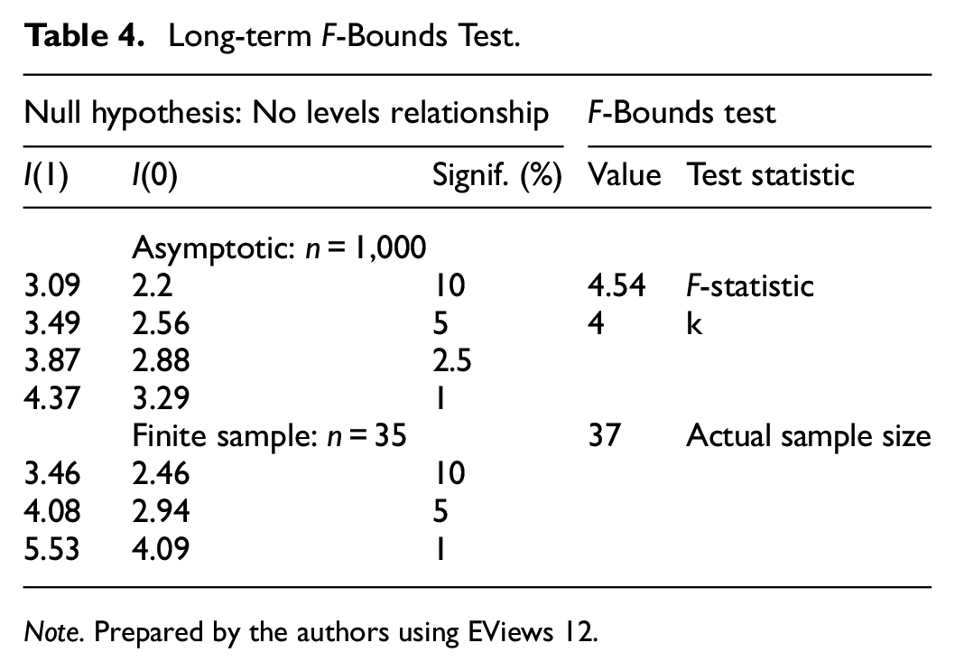
Note. Prepared by the authors using EViews 12.

Table 4 implies a long-term cointegration relationship between the independent and dependent variables, as indicated by the F-Bounds Test statistic, which is greater than the critical value at a significance level of 5%. This suggests that there is a cointegration relationship between the variables in the long term. Table 5 shows the long-term ARDL Bounds test model in constant and without trend (case 2).

Table 5.

Estimating the ARDL Model (2,1,2,1,2) in the Long Term.

Levels equation
Variable	Coefficient	Std. error	t-Statistic	Prob.
Government Revenue	0.262	0.154	1.70	0.102
INF	2.99	0.95	3.12	0.00***
External Debt	0.172	0.090	1.90	0.069*
Total Government Expenditure	0.563	0.123	4.56	0.00***
C	−16.22	1.86	−8.69	0.00***

Note.***, **, * imply significance at the 1%, 5%, and 10% level, respectively. Prepared by the authors using EViews 12.

From Table 5, it is found that government revenues do not have a significant impact on economic growth in the long term. Additionally, it is noted that total government expenditure has a positive and statistically significant effect at the 1% level, where a 1% increase in total government spending leads to a 0.56% increase in long-term economic growth, with all other factors held constant. Also, external debt has a positive and statistically significant effect at the 10% level,¹ where a 1% increase in external debt leads to a 0.17% increase in long-term economic growth, with all other factors held constant. This suggests that external debt is sustainable in Egypt and within safe limits. Additionally, the effect of the inflation rate is positive and statistically significant at the 1% level, where a 1% increase in the inflation rate leads to a 2.99% increase in long-term economic growth, with all other factors held constant. This is consistent, given that economic growth was measured at current prices.

Estimating the Relationship in the Short Term

After confirming the cointegration between the study variables, we move to the UECM model, shown in Table 6.

Table 6.

Estimating the ARDL Model (2,1,2,1,2) in the Short Term.

UECM regression
Variable	Coefficient	Std. error	t-Statistic	Prob.
Δ (GDP Per Capita (-1))	0.447	0.09	4.65	0.00^***
Δ (Total Government Expenditure)	−0.104	0.055	−1.90	0.06^*
Δ (Revenue)	0.046	0.025	1.80	0.08^*
Δ (Revenue (-1))	−0.08	0.032	−2.44	0.02^**
Δ (External Debt)	−0.039	0.02	−1.94	0.06^*
Δ (INF)	0.92	0.04	20.64	0.00^***
Δ (INF (−1))	−0.124	0.04	−2.90	0.00^***
Dummy	0.065	0.010	6.17	0.00^***
CointEq(−1)*	−0.216	0.03	−6.36	0.00^***

Note.***, **, * imply significance at the 1%, 5%, and 10% level, respectively. Prepared by the authors using EViews 12.

The findings presented in Table 6 indicate a significant negative error correction coefficient at the 1% significance level. This suggests the presence of a long-term cointegration relationship between the independent variables and the dependent variable. The coefficient value of −0.216 is less than one, indicating that the dependent variable returns to its equilibrium position at a speed of approximately four and a half years. In each period, the previous period’s imbalance ratio (t − 1) is estimated at −0.216. This means that 21.6% of this imbalance is corrected during the period t (in 1 year) until it reaches the long-term equilibrium after approximately 4.62 years.

Moreover, GDP per capita (−1) has a positive and statistically significant impact on economic growth in the current year, with a 1% increase in GDP per capita resulting in a 0.44% increase in economic growth in the short term, holding all other factors constant. On the other hand, an increase in government revenues in the previous year led to a decrease of −0.08% in economic growth in the current year in the short term, with all other factors held constant. This highlights the need for reform in government revenue policies to promote sustainable economic growth and resilience to shocks. Furthermore, the previous year’s inflation rate has a negative and statistically significant effect of 1% on economic growth in the current year, with a 1% increase in inflation rate resulting in a decrease of −0.12% in economic growth in the short term, holding all other factors constant. Lastly, the dummy variable representing structural changes has a positive and statistically significant impact in the short term on economic growth.

Diagnostic Tests

Table 7 shows several diagnostic tests to verify the quality of the model.

Table 7.

Diagnostic Tests for the ARDL Form (2,1,2,1,2).

Normality test (Jarque-Bera)	X²	0.62	Prob.	0.73
Breusch-Godfrey Serial Correlation (LM test)	F-statistic	0.37	Prob. F(2,21)	0.68
Breusch-Godfrey Serial Correlation (LM test)	Obs × R-squared	1.29	Prob.ChiSquare(2)	0.52
ARCH (heteroskedasticity test)	F-statistic	0.72	Prob. F(2,32)	0.49
ARCH (heteroskedasticity test)	Obs × R-squared	1.51	Prob.ChiSquare(2)	0.46
Ramsey RESET test	F-statistic	0.11	Probability	0.74
Ramsey RESET test	t-Statistic	0.33	Probability	0.74

Source. Prepared by the authors using EViews 12.

Note.***, **, * imply significance at the 1%, 5%, and 10% level, respectively.

The ARDL model diagnostic tests ensure it is free of serial autocorrelation and heteroscedasticity and that the CUSUM graph has significant stability (i.e., lies between the two-bonded lines at a 5% level of significance). From Table 7, The Jarque-Bera test, which assesses the normality of the residuals, had a p-value of .73. Since this value is >.05, we cannot reject the null hypothesis that the residuals follow a normal distribution (Jarque & Bera, 1980). The Breusch-Godfrey Serial Correlation test, which checks for autocorrelation in the residuals, had a p-value of .68. This value indicates that we cannot reject the null hypothesis of no serial correlation (Breusch, 1978). The ARCH test, which checks for heteroskedasticity in the residuals, had a p-value of .69. This value indicates we cannot reject the null hypothesis of no heteroscedasticity (Engle, 1982). The Ramsey RESET test, which checks for omitted variable bias, had a p-value of .74. This value indicates we cannot reject the null hypothesis of no omitted variable bias. Overall, these results suggest that the model does not suffer from problems of normality, autocorrelation, heteroskedasticity, or omitted variable bias. This suggests that the model is well-specified and can be used for further analysis (Ramsey, 1969).

Following the estimation of the error correction equation for the ARDL model, the next step is to evaluate the structural stability of short- and long-term parameters through two tests, the Cumulative Sum of Recursive Residual (CUSUM) test and the Cumulative Sum of Square Recursive Residual (CUSUMSQ) test (Brown et al., 1975). These tests are employed to ascertain if the coefficients estimated in the error correction equation of the ARDL model remain stable over time. The coefficients are structurally stable if the CUSUM and CUSUMSQ statistics plots stay within the critical lines at a significance level of 5%. Conversely, if the plots of the CUSUM and CUSUMSQ statistics are outside the critical lines, it implies that the coefficients are not stable. To confirm that the data used in the research is free of any structural changes and to determine the stability and consistency of long-term coefficients with estimates of short-term coefficients, both the CUSUM test and CUSUMSQ test graphs are located within the critical limits at the 5% significance level, which demonstrates the stability and consistency of the model’s estimates between the short-term and long-term results. Therefore, the model is free from econometric problems and can be accepted.

Discussion

This study found a dynamic and equilibrium relationship between fiscal sustainability indicators and economic growth in Egypt in the short and long term. This supports the view that Egypt’s fiscal policy is sustainable, consistent with previous studies. For instance, Al Sayed et al. (2021) used a cointegration analysis to show that the fiscal policy in Egypt was sustainable from 1990/1991 to 2017/2018. Similarly, Abdullah et al. (2012) found a cointegration between fiscal sustainability indicators and GDP in Malaysia, indicating fiscal sustainability. The results of our study offer valuable insights into the impact of different factors on economic growth in Egypt, which can inform policymaking and future research. The study found that government revenues do not significantly impact long-term economic growth in Egypt, in contrast to some other studies that have reported a negative impact (Benazić, 2006; Dang, 2013; Karras & Furceri, 2009; Marimuthu et al., 2021) or positive effects (Gray et al., 2007). This difference highlights the need to understand better the specific context in which fiscal policies are implemented. In Egypt’s case, the positive and statistically significant effect of total government expenditure on economic growth can be attributed to the country’s ongoing efforts to control public spending and stimulate growth. A 1% increase in government spending leads to a 0.56% increase in long-term economic growth. This is consistent with the findings of Barro (1990), which demonstrate a direct and statistically significant association between government spending and economic growth. The positive effect of government spending on economic growth may be due to the reforms implemented in Egypt to control public spending and stimulate economic growth. These findings are consistent with the findings of Al Khatib et al. (2022), Agu et al. (2015), Chang et al. (2011), Wu et al. (2010), and J. C. Lee et al. (2019).

Moreover, the analysis revealed that external debt is positively and statistically significant in impacting economic growth. A 1% increase in external debt leads to a 0.17% increase in long-term economic growth, indicating that external debt can drive economic growth by increasing capital flows and supporting productive projects. This finding is consistent with the Keynesian view and other studies, such as Eberhardt and Presbitero (2015). Nevertheless, the implications of external debt on economic growth may vary depending on economic conditions and policy environments, as evidenced by Asteriou et al. (2021) results.

The inflation rate was also found to positively and statistically significantly affect economic growth. This is consistent with theories that higher inflation decreases the real value of money, increasing investment and economic growth (Mallik & Chowdhury, 2001; Mundell, 1963; Tobin, 1965). However, inflation’s impact on economic growth is complex and depends on country-specific factors.

The UECM model shows that economic growth converges to equilibrium in about 4.5 years. This suggests that policy effects on economic growth may emerge over several years. The model also shows that effects on economic growth may differ in the short and long run, highlighting the need to monitor relationships over time to inform policy. The UECM conditional error correction model results provided further insights into the impact of the variables in the short term, showing that economic growth, government revenues, inflation, and structural changes in the previous year significantly impact current economic growth. These findings highlight the importance of considering long-term and short-term factors in policymaking and the need for targeted reforms to stimulate sustainable economic growth in Egypt.

The UECM conditional error correction model presented in Table 6 further supports the finding that GDP per capita in the previous year has a positive and statistically significant effect on economic growth in the current year; a 1% increase in economic growth in the previous year leads to a 0.44% increase in economic growth in the current year. On the other hand, government revenues in the previous year have a negative and statistically significant effect on economic growth in the current year, with a 1% increase in government revenues leading to a −0.08% decrease in economic growth in the current year. This finding is consistent with the results of a previous study (Benazić, 2006).

Similarly, the inflation rate in the previous year is found to have a negative and statistically significant effect on economic growth in the current year, with a 1% increase in the inflation rate leading to a −0.12% decrease in economic growth in the current year. This finding agrees with Datta and Mukhopadhyay (2011) and Faria and Carneiro (2001) findings which showed a short-run negative relationship between inflation and economic growth. However, the two variables were positively related in the long run (Datta & Mukhopadhyay, 2011). It is common for a negative relationship between inflation and economic growth in the short run but a positive relationship in the long run. This is because high inflation levels can negatively affect economic activity in the short run, such as reducing consumer and business confidence, increasing uncertainty, and disrupting financial markets. However, in the long run, the relationship between inflation and economic growth may become positive, as the negative effects of inflation tend to dissipate and the positive effects of investment and economic expansion take hold. The results of the UECM model also indicate that structural changes, as captured by the dummy variable, have a positive and statistically significant effect on economic growth in the current year. It is common for structural changes, such as economic policy, regulatory frameworks, or technological developments, to impact economic growth. These changes can affect the production and distribution of goods and services and the level of investment and productivity in an economy. If favorable structural changes increase efficiency, they may positively affect economic growth. Overall, the analysis suggests that total government expenditure and external debt positively impact economic growth in the long term. In addition, GDP per capita, government revenues, and the inflation rate positively or negatively affect economic growth in the short term. The findings highlight the importance of considering both long-term and short-term factors in policymaking and the need for reform in specific areas, such as government revenues, to sustainably stimulate economic growth in Egypt.

Conclusion

The findings of this study suggest that total government expenditure and external debt positively impact economic growth in the long term. However, GDP per capita, government revenues, and inflation rate can have varying effects on economic growth in the short term. These results emphasize the importance of ongoing monitoring and analysis of the relationship between different factors and economic growth to inform policy decisions and ensure sustainable economic development in Egypt. Moreover, this study contributes to the existing literature by providing empirical evidence on the long-term effects of government expenditure, government revenue, and external debt on economic growth in Egypt, which previous studies have largely neglected.

Policy Implications

Based on the findings of this study, Prudent fiscal management is crucial for sustained economic development. Policymakers should focus on controlling government spending, limiting external debt, and improving revenue generation to promote long-term economic growth in Egypt. Fiscal sustainability must balance critical investments in public services. Carefully managing fiscal deficits is vital to unleashing Egypt’s economic potential. Policymakers should consider both short and long-term effects when making fiscal policy decisions. In particular, they should reform government revenues to sustainably stimulate economic growth, as higher revenues can reduce the need for borrowing or taxation. They should also carefully weigh the benefits and costs of increasing government expenditure and external debt, as they may entail trade-offs such as higher taxes or less spending elsewhere. Furthermore, they should manage external debt prudently to avoid excessive debt service payments that can strain the country’s budget and limit its fiscal space. Additionally, policymakers should use fiscal policy to support other aspects of sustainable development, such as environmental protection and social welfare. For instance, they can use fiscal incentives to promote forest conservation and ecosystem health, vital for climate stability and reducing the risk of zoonotic diseases. They can also use fiscal transfers to improve the poor and vulnerable groups’ living standards and human capital. Therefore, fiscal policy is a core component of governmental interventions that can influence Egypt’s development path and growth rate.

Study Limitations

This study has some limitations that should be acknowledged. First, it may have omitted some relevant factors that affect economic growth in Egypt, such as trade policies, human capital, and technological progress. Second, it may have been subject to measurement errors or omitted variable bias due to data limitations or model specifications. Third, it may not be generalizable to other countries or regions due to Egypt’s unique economic conditions and policy environment.

Future Research Directions

Future research should address these limitations by examining the impact of additional factors on economic growth, extending the analysis to other countries or regions, and refining the methodology to minimize potential biases. For example, future research can use panel data analysis or instrumental variable estimation to account for unobserved heterogeneity or endogeneity issues. Future research can also explore the nonlinear or threshold effects of government expenditure and external debt on economic growth and their interactions with other variables. Furthermore, future research can compare and contrast the effects of government expenditure and external debt on economic growth, such as productive versus unproductive spending or concessional versus non-concessional debt.

Footnotes

Declaration of Conflicting Interests

The author(s) declared no potential conflicts of interest with respect to the research, authorship, and/or publication of this article.

Funding

The author(s) received no financial support for the research, authorship, and/or publication of this article.

Ethics Statement

Not applicable.

ORCID iD

Alina Cristina Nuta

Data Availability Statement

Data sharing not applicable to this article as no datasets were generated or analyzed during the current study.

Notes

References

Abdullah

Mohd

M. M.

Dahalan

(2012). An empirical study on fiscal sustainability in Malaysia. International Journal of Academic Research in Business and Social Sciences, 2(1), 72–90.

Afonso

Furceri

(2010). Government size, composition, volatility and economic growth. European Journal of Political Economy, 26, 517–532. https://doi.org/10.1016/j.ejpoleco.2010.02.002

Agu

S. U.

Okwo

I. M.

Ugwunta

O. D.

Idike

(2015). Fiscal policy and economic growth in Nigeria: Emphasis on various components of public expenditure. Sage Open, 5(4), 1–12. https://doi.org/10.1177/2158244015610171

Akyüz

(2007). Debt sustainability in emerging markets: A critical appraisal (p. 61). Economic & Social Affairs.

Algaeed

A. H.

(2022). Government spending volatility and real economic growth: Evidence from a major oil producing country, Saudi Arabia, 1970 to 2018. Sage Open, 12(2), 1–13. https://doi.org/10.1177/21582440221089948

Ali

Irfan

Ozturk

Rauf

(2023). Modeling public acceptance of renewable energy deployment: A pathway towards green revolution. Economic Research-Ekonomska Istraživanja, 36, 1–19. https://doi.org/10.1080/1331677x.2022.2159849

Ali

Yan

Dilanchiev

Irfan

Fahad

(2022). Modeling the economic viability and performance of solar home systems: A roadmap towards clean energy for environmental sustainability. Environmental Science and Pollution Research, 30, 30612–30631. https://doi.org/10.1007/s11356-022-24387-6

Al Khatib

A. M. G.

Alshaib

B. M.

Mishra

Narvariya

R. K.

Yadav

Ray

Kanaan

(2022). Modeling and analyzing the dynamic impact of financial development on economic growth in syria. Economic Affairs, 67(5), 855–897. https://doi.org/10.46852/0424-2513.5.2022.24

Al Khatib

A. M. G.

Pawariya

Lal

Ray

Mishra

Kumar

Ali Kanaan

(2023). The relationship between financial development and inflation rate in Egypt. Indian Journal of Economics and Development, 19(1), 17–31. https://doi.org/10.35716/ijed/22298

10.

Al Sayed

Samir

Anwar

H. H.

(2021). Assessing fiscal sustainability in Egypt: A comparative study. Review of Economics and Political Science, 6(4), 292–310. https://doi.org/10.1108/reps-02-2020-0020

11.

Al-Shawarby

Alba

Iqbal

(2004). Fiscal and public debt sustainability in Egypt (English). Middle East and North Africa (Working Paper Series; no. MNA 38). World Bank Group. http://documents.worldbank.org/curated/en/587421468770130638/Fiscal-and-public-debt-sustainability-in-Egypt

12.

Amsler

Lee

(1995). An LM test for a unit root in the presence of a structural change. Economic Theory, 11(2), 359–368.

13.

Asif

M. H.

Zhongfu

Ahmad

Irfan

Razzaq

Ameer

(2022). Influencing factors of consumers’ buying intention of solar energy: A structural equation modeling approach. Environmental Science and Pollution Research, 30, 30017–30032. https://doi.org/10.1007/s11356-022-24286-w

14.

Asif

M. H.

Zhongfu

Dilanchiev

Irfan

Eyvazov

Ahmad

(2023). Determining the influencing factors of consumers’ attitude toward renewable energy adoption in developing countries: A roadmap toward environmental sustainability and green energy technologies. Environmental Science and Pollution Research, 30, 47861–47872. https://doi.org/10.1007/s11356-023-25662-w

15.

Asteriou

Pilbeam

Pratiwi

C. E.

(2021). Public debt and economic growth: Panel data evidence for Asian countries. Journal of Economics and Finance, 45(2), 270–287. https://doi.org/10.1007/s12197-020-09515-7

16.

Awad

I. M.

Al-Jerashi

G. K.

Alabaddi

Z. A.

(2021). Determinants of private domestic investment in Palestine: Time series analysis. Journal of Business and Socio-economic Development, 1(1), 71–86. https://doi.org/10.1108/jbsed-04-2021-0038

17.

Ayad

Mishra

Kumari

Ray

Nuţă

F. M.

Gautam

Balsalobre-Lorente

Nuţă

A. C.

Zamfir

C. G.

(2023). The spillover effects of uncertainty and globalization on environmental quality in India: Evidence from combined cointegration test and augmented ARDL model. Frontiers in Environmental Science, 11, 1144201. https://doi.org/10.3389/fenvs.2023.1144201

18.

Ayadi

F. S.

Ayadi

F. O.

(2008). The impact of external debt on economic growth: A comparative study of Nigeria and South Africa. Journal of sustainable development in Africa, 10(3), 234–264.

19.

Ayumu

(2004). Fiscal Sustainability-the Case of Eritrea (IMF Working).

20.

Barro

R. J.

(1990). Government spending in a simple model of endogeneous growth. Journal of Political Economy, 98(5, Part 2), S103–S125. https://doi.org/10.1086/261726

21.

Benazić

(2006). Fiscal policy and economic activity in the Republic of Croatia: A Cointegration analysis. Ekonomski Pregled, 57(12), 882–917.

22.

Breusch

T. S.

(1978). Testing for autocorrelation in dynamic linear models. Australian Economic Papers, 17(31), 334–355. https://doi.org/10.1111/j.1467-8454.1978.tb00635.x

23.

Brown

R. L.

Durbin

Evans

J. M.

(1975). Techniques for testing the constancy of regression relationships over time. Journal of the Royal Statistical Society, 37(2), 149–163.

24.

Bruni

(2017). Egypt labour market report: Demographic trends, labour market evolution and scenarios for the period 2015–2030. International Organization for Migration. Retrieved November 01, 2022, from https://publications.iom.int/system/files/pdf/egypt_labour_market_report.pdf

25.

CB. (2015). Central Bank of Egypt, Annual Report 2014/2015. Author. https://cbe.org.eg/en/EconomicResearch/Publications/AnnualReportDL/Annual%20Report2014-2015.pdf; https://cbe.org.eg/-/media/project/cbe/listing/

26.

Chalk

N. A.

Hemming

(2000). Assessing fiscal sustainability in theory and practice (IMF Working).

27.

Chang

H.-C.

Huang

B.-N.

Yang

C. W.

(2011). Military expenditure and economic growth across different groups: A dynamic panel Granger-causality approach. Economic Modelling, 28, 2416–2423. https://doi.org/10.1016/j.econmod.2011.06.001

28.

Cigu

Petrişor

M. B.

Nuţă

A. C.

Nuţă

F. M.

Bostan

(2020). The nexus between financial regulation and Green Sustainable Economy. Sustainability, 12(21), 8778. https://doi.org/10.3390/su12218778

29.

Coman Nuţă

A. C.

Lupu

Nuţă

F. M.

(2023). The impact of public education spending on economic growth in Central and Eastern Europe. An ARDL approach with structural break. Economic Research-Ekonomska Istraživanja, 36(1), 1261–1278. https://doi.org/10.1080/1331677X.2022.2086147

30.

Dang

D. Y.

(2013). Revenue allocation and economic development in Nigeria: An empirical study. Sage Open, 3(3), 1–7. https://doi.org/10.1177/2158244013505602

31.

Datta

Mukhopadhyay

C. K.

(2011). Relationship between inflation and economic growth in Malaysia-An econometric review [Conference session]. International Conference on Economics and Finance Research.

32.

Dickey

D. A.

Fuller

W. A.

(1981). Likelihood ratio statistics for autoregressive time series with a unit root. Econometrica, 49, 1057–1072. https://doi.org/10.2307/1912517

33.

Domar

E. D.

(1944). The “burden of the debt” and the national income. American Economic Review, 34(4), 798–827.

34.

Dudzevičiūtė

Šimelytė

Liučvaitienė

(2018). Government expenditure and economic growth in the European Union countries. International Journal of Social Economics, 45, 372–386.

35.

Durevall

Henrekson

(2011). The futile quest for a grand explanation of long-run government expenditure. Journal of Public Economics, 95, 708–722. https://doi.org/10.1016/j.jpubeco.2011.02.004

36.

Eberhardt

Presbitero

A. F.

(2015). Public debt and growth: Heterogeneity and non-linearity. Journal of International Economics, 97(1), 45–58. https://doi.org/10.1016/j.jinteco.2015.04.005

37.

El Husseiny

I. A.

(2020). Enhancing the role of fiscal policy in achieving the sustainable development goals (SDGs): Insights from behavioral economics with a special reference to Egypt. Journal of Economics Finance and Administrative Science, (106), 22–43.

38.

Engle

R. F.

(1982). Autoregressive conditional heteroscedasticity with estimates of the variance of United Kingdom inflation. Econometrica, 50(4), 987. https://doi.org/10.2307/1912773

39.

Faria

J. R.

Carneiro

F. G.

(2001). Does high inflation affect growth in the long and short run? Journal of Applied Economics, 4(1), 89–105. https://doi.org/10.1080/15140326.2001.12040559

40.

Farouk

(2014). More than money: Post-mubarak Egypt, Saudi Arabia, and the Gulf (pp. 1–24). Gulf Research Center.

41.

Fathy Abdelgany

Badr Al-deen

(2023). Constraints to debt sustainability in Egypt: Structural response and fiscal fatigue. International Journal of Economics Finance and Management Sciences, 11(2), 44–61. https://doi.org/10.11648/j.ijefm.20231102.12

42.

Gao

Liu

Dong

(2021). Does air pollution impact fiscal sustainability? Evidence from Chinese cities. Energies, 14, 7247. https://doi.org/10.3390/en14217247

43.

Gómez-Puig

Sosvilla-Rivero

(2015). Short-run and long-run effects of public debt on economic performance: Evidence from EMU countries. Available at SSRN 2660117.

44.

Gray

C. W.

Lane

Varoudakis

(2007). Fiscal policy and economic growth: Lessons for Eastern Europe and Central Asia. World Bank Publications. https://openknowledge.worldbank.org/handle/10986/6883

45.

Gregory

A. W.

Hansen

B. E.

(1996a). Residual-based tests for cointegration in models with regime shifts. Journal of Econometrics, 70(1), 99–126. https://doi.org/10.1016/0304-4076(69)41685-7

46.

Gregory

A. W.

Hansen

B. E.

(1996b). Practitioners corner: Tests for cointegration in models with regime and trend shifts. Oxford Bulletin of Economics and Statistics, 58(3), 555–560. https://doi.org/10.1111/j.1468-0084.1996.mp58003008.x

47.

Hakkio

C. S.

Rush

(1991). Is the budget deficit too large? Economic Inquiry, 29(3), 429–445. https://doi.org/10.1111/j.1465-7295.1991.tb00837.x

48.

Hussain

Ali

Ahmad

(2021). A dynamic analysis of the impact of fiscal adjustment on economic growth: Evidence from Pakistan. Sage Open, 11(2), 1–19. https://doi.org/10.1177/21582440211027167

49.

Jarque

C. M.

Bera

A. K.

(1980). Efficient tests for normality, homoscedasticity and serial independence of regression residuals. Economics Letters, 6(3), 255–259. https://doi.org/10.1016/0165-1765(80)90024-51980.

50.

Johansen

(1991). Estimation and hypothesis testing of cointegration vectors in Gaussian vector autoregressive models. Econometrica, 59, 1551–1580. https://doi.org/10.2307/2938278

51.

Karras

Furceri

(2009). Taxes and growth in Europe. South-Eastern Europe Journal of Economics, 7(2), 181–204.

52.

Kathomi

Maina

K. E.

Kariuki

S. N.

(2017). Interest rate regulation and sustainability of microfinance institutions in Nairobi Country Kenya. International Academic Journal of Human Resource and Business Administration, 2(3), 150–165.

53.

Kluza

(2016). Sustainability of local government sector debt. Evidence from Monte-Carlo simulations. Lex localis - Journal of Local Self Government, 14, 115–132. https://doi.org/10.4335/115-132

54.

Lee

Strazicich

M. C.

(2003). Minimum Lagrange multiplier unit root test with two structural breaks. Review of Economics and Statistics, 85(4), 1082–1089.

55.

Lee

J. C.

Won

Y. J.

Jei

S. Y.

(2019). Study of the relationship between government expenditures and economic growth for China and Korea. Sustainability, 11, 6344. https://doi.org/10.3390/su11226344

56.

Lestari

(2014). Can Indonesia’s fiscal policy be sustained, with exploding debt (No. 201415). Department of Economics, Padjadjaran University.

57.

Lobont

O. R.

Moldovan

N. C.

Bociu

Chis

Brindescu Olariu

(2018). A factor analysis of the public sector performance. Significant differences between Old and new EU countries. Economic Computation and Economic Cybernetics Studies and Research/Academy of Economic Studies, 52(2), 139–156.

58.

López Subires

M. D.

Alcaide Muñoz

Navarro Galera

Rodríguez Bolívar

M. P.

(2019). The influence of socio-demographic factors on financial sustainability of public services: A comparative analysis in regional governments and local governments. Sustainability, 11, 6008. https://doi.org/10.3390/su11216008

59.

Lumsdaine

R. L.

Papell

D. H.

(1997). Multiple trend breaks and the unit-root hypothesis. Review of Economics and Statistics, 79(2), 212–218.

60.

Maki

(2012). Tests for cointegration allowing for an unknown number of breaks. Economic Modelling, 29(5), 2011–2015. https://doi.org/10.1016/j.econmod.2012.04.022

61.

Mallik

Chowdhury

(2001). Inflation and economic growth: Evidence from four south Asian countries. Asia-Pacific Development Journal, 8(1), 123–135.

62.

Marimuthu

Khan

Bangash

(2021). Is the fiscal deficit of ASEAN alarming? Evidence from fiscal deficit consequences and contribution towards sustainable economic growth. Sustainability, 13, 10045. https://doi.org/10.3390/su131810045

63.

Martin

G. M.

(2000). US deficit sustainability: A new approach based on multiple endogenous breaks. Journal of Applied Economics, 15(1), 83–105.

64.

Méndez-Marcano

Pineda

(2008). Fiscal sustainability and economic growth in bolivia. BBVA.

65.

Moldovan

N. C.

Hatmanu

Lobont

O. R.

(2014). Reflections on the Romanian fiscal policy-driven election manipulation phenomenon. Economic Computation and Economic Cybernetics Studies and Research/Academy of Economic Studies, 48(2), 91–112.

66.

Mundell

(1963). Inflation and real interest. Journal of Political Economy, 71(3), 280–283.

67.

Narayan

P. K.

(2005). The saving and investment nexus for China: Evidence from cointegration tests. Applied Economics, 37(17), 1979–1990. https://doi.org/10.1080/00036840500278103

68.

Narayan

P. K.

Popp

(2010). A new unit root test with two structural breaks in level and slope at unknown time. Journal of Applied Statistics, 37(9), 1425–1438. https://doi.org/10.1080/02664760903039883

69.

New Zealand Treasury. (2013). Affording our future; Statement on New Zealand’s long-term fiscal position. Author. http://www.treasury.govt.nz/government/longterm/fiscalposition/2013/affordingourfuture/ltfs-13-aof.pdf

70.

Nuţă

A.-C.

Nuţă

F.-M.

(2020). Modelling the influences of economic, demographic, and institutional factors on fiscal pressure using OLS, PCSE, and FD-GMM approaches. Sustainability, 12(4), 1681. https://doi.org/10.3390/su12041681

71.

Nuţă

A. C.

Nuţă

F. M.

Chirilă

Roman

Puşcă

A. C.

(2015). Testing the relationship between public expenditure and economic growth in Romania. ACTA Universitates Danubius, 11(4), 86–102.

72.

Nyasha

Odhiambo

N. M.

(2019). Government size and economic growth: A review of international literature. Sage Open, 9(3), 1–12. https://doi.org/10.1177/2158244019877200

73.

Perron

(1997). Further evidence on breaking trend functions in macroeconomic variables. Journal of Econometrics, 80(2), 355–385. https://doi.org/10.1016/s0304-4076(97)00049-3

74.

Perron

Vogelsang

T. J.

(1992). Nonstationarity and level shifts with an application to purchasing power parity. Journal of Business and Economic Statistics, 10(3), 301. https://doi.org/10.2307/1391544

75.

Pesaran

M. H.

Shin

Smith

R. J.

(2001). Bounds testing approaches to the analysis of level relationships. Journal of Applied Econometrics, 16(3), 289–326.

76.

Quintos

C. E.

(1995). Sustainability of the deficit process with structural shifts. Journal of Business and Economic Statistics, 13(4), 409–417. https://doi.org/10.1080/07350015.1995.10524615

77.

Ramsey

J. B.

(1969). Tests for specification errors in classical linear least-squares regression analysis. Journal of The Royal Statistical Society, 31(2), 350–371. https://doi.org/10.1111/j.2517-6161.1969.tb00796.x

78.

Rodríguez Bolívar

Navarro Galera

Alcaide Muñoz

López Subires

M. D.

(2016). Analyzing forces to the financial contribution of local governments to sustainable development. Sustainability, 8, 925. https://doi.org/10.3390/su8090925

79.

Rose

(2010). Institutions and fiscal sustainability. National Tax Journal, 63(4.1), 807–837.

80.

Samudram

Nair

Vaithilingam

(2009). Keynes and Wagner on government expenditures and economic development: The case of a developing economy. Empirical Economics, 36, 713–712. https://doi.org/10.1007/s00181-009-0264-z

81.

Ţibulcă

I.-L.

(2021). Debt sustainability: Can EU member states use environmental taxes to regain fiscal space? Sustainability, 13, 5952. https://doi.org/10.3390/su13115952

82.

Tobin

(1965). Money and economic growth. Econometrica, 33, 671–684. https://doi.org/10.2307/1910352

83.

Verbeek

(2004). A guide to modern econometrics. John Wiley & Sons Ltd.

84.

S.-Y.

Tang

J.-H.

Lin

E. S.

(2010). The impact of government expenditure on economic growth: How sensitive to the level of development? Journal of Policy Modeling, 32, 804–817. https://doi.org/10.1016/j.jpolmod.2010.05.011

85.

Zeeshan

Han

Rehman

Ullah

Hussain

Alam Afridi

F. E.

, (2022). Exploring symmetric and asymmetric nexus between corruption, political instability, natural resources and economic growth in the context of Pakistan. Resources Policy, 78, 102785. https://doi.org/10.1016/j.resourpol.2022.102785

86.

Zhang

Nuţă

F. M.

Dimen

Ullah

Xuanye

Junchen

Yihan

(2023). Relationship between FDI inflow, CO2 emissions, renewable energy consumption, and population health quality in China. Frontiers in Environmental Science, 11, 99. https://doi.org/10.3389/fenvs.2023.1120970

87.

Zivot

Andrews

D. W. K.

(2002). Further evidence on the great crash, the oil-price shock, and the unit-root hypothesis. Journal of Business and Economic Statistics, 20(1), 25–44. https://doi.org/10.1198/073500102753410372

Fiscal Sustainability and Its Implications for Economic Growth in Egypt: An Empirical Analysis

Abstract

Plain Language Summary

Keywords

Introduction

Literature Review

Theoretical Overview

Fiscal Sustainability Indicators

Factors Affecting Fiscal Sustainability

Empirical Overview

Fiscal Sustainability in Egypt

Research Methodology

Unit Root Tests

Cointegration Analysis Using Pesaran et al. (2001) Approach

Conditional Error Correction Model (UECM)

Stability and Diagnostic Test

Unit Root Tests

Cointegration Analysis Using Pesaran (2001) Approach

Bounds Test Approach

Stability and Diagnostic Test

Data

Research Variables

Dependent variable

Independent Variables

Total Government Expenditure

Government Revenue Excluding Grants

Total External Debt

Inflation Rate

Dummy Variable

Results

Estimation of the ARDL Bounds Test Model

Estimating the Relationship in the Short Term

Diagnostic Tests

Discussion

Conclusion

Policy Implications

Study Limitations

Future Research Directions

Footnotes

Declaration of Conflicting Interests

Funding

Ethics Statement

ORCID iD

Data Availability Statement

Notes

References