Economic Growth in Saudi Arabia through Sectoral Reallocation of Government Expenditures

Abstract

The article employs auto-regressive distributed lag (ARDL) cointegration and error-correction modelling to study the long-run impact of investment, exports, imports, and three components of government expenditures (expenditures on health, education, and other government spending) on GDP growth in Saudi Arabia from 1985 to 2018. We observe the long-run positive relationship between GDP, investment, exports and government education expenditure, but a negative relationship between GDP, imports, government health spending, and government other expenditures. The analysis reveals that investment, exports, and government educational expenditures all have long-run positive effects on the GDP growth, while imports, government health expenditures, and government other expenditures negatively affect GDP growth in Saudi Arabia. The Toda-Yamamoto causality test that applies the Modified Wald test establishes causality from exports, government education spending, and government health spending to GDP. We deduce that education expenditures stimulate economic growth in Saudi Arabia in contrast to health expenditures. Additionally, we infer that the various categories of government expenditures have varying effects on GDP. This necessitates a prudent sectoral allocation of public expenditures to maximize its positive effects on GDP growth and stimulate economic growth in Saudi Arabia. Moreover, the above findings have policy implications for the government in Saudi Arabia while allocating its expenditures. Allocating more government expenditures to education, cutting down inessential spending, and downsizing government healthcare expenditures will enhance long-run economic growth in Saudi Arabia.

JEL Classification: O470; I15; I25

Introduction

A country’s principal macroeconomic objective is to achieve a high economic growth rate. Economic growth is a critical indicator of a nation’s overall financial health (Abid, 2020). Demand-side economic theories advocate for government spending for boosting a country’s economic growth. However, there is no widespread agreement among researchers on this point. On the one hand, the Keynesian view emphasizes the size of government spending and views it as a cause of economic growth, not the reverse (Chu et al., 2020; Ebaidalla, 2013; Loizides & Vamvoukas, 2005). On the other hand, Wagner’s Law explains that while the size of government expenditures increases as an economy expands, it does not result in economic growth due to an economy’s inefficient use of its resources (Islam, 2001; Thabane & Lebina, 2016). Certain middle views assert a bidirectional causal linkage between economic growth and government outlays (Abu-Eideh, 2015; Wu et al., 2010). Thus, empirical corroboration on the connection between government expenditure and economic growth is contradictory, contentious, inconclusive, and varies from country to country.

A nation’s people and economic resources mostly determine its economic growth and progress. However, the people of a country play a vital part in making the optimum use of the country’s limited resources. The education, knowledge, and training called human capital largely influence people’s ability to effectively use scarce resources and achieve rapid growth, development, and technological breakthroughs. Education is critical to a country’s socio-economic development. Education contributes to a country’s eradication of crime, poverty, unemployment, and disease. Additionally, it contributes significantly to technological breakthroughs and teaches various skills important for a nation’s economic development.

Realizing the critical role education plays in developing a country, Saudi Arabia began developing various types of educational infrastructures on a large scale in the late 1990s. Since then, education expenditures have accounted for a sizable portion of its total public expenditures. In real terms, Saudi Arabia’s total government expenditure was 31.9% of GDP in 1985, which slightly decreased to 24.6% in 2018. Despite this decline in total government spending, education spending increased from 5.3% of GDP in 1985 to 7.5% in 2018. Additionally, the share of education spending in total government spending increased significantly from 16.7% in 1985 to 30.7% in 2018. This demonstrates that Saudi Arabia invests heavily in education to increase human capital and develop its human resources to meet its demand for an educated workforce for various purposes. As far as government health expenditure is concerned, it was only 1.83% of GDP in 1985, which rose to 3.19% of GDP in 2018. Government expenditure on health as a percentage of government total expenditures was 5.72% in 1985, which jumped to 12.94% in 2018 (www.sama.gov.sa). These data on government expenditure and its each expenditure category is published by the Saudi Arabian Monetary Agency (SAMA) at current prices. We converted them at constant prices using GDP deflator and then we calculated expenditures in percentage. In this pandemic era, the efficiency and effectiveness of a country’s health sector will considerably determine the economic growth performance of that country during the pandemic years and in the years after it.

We believe that, among other things, higher economic growth can also be realized through proper channelling the government revenue in various sectors. Government expenditures are diverse and can be broken down into numerous components, each of which can affect a nation’s economic growth. Given Saudi Arabia’s large educational expenditures, it is vital to analyze if they are contributing to the nation’s economic growth.

Therefore, the principal goal of this study is to investigate the influence of three major components of total government spending in Saudi Arabia: education, health, and all other expenditures, which we term as government other expenditures. Moreover, we aim to find out whether proper sectoral re-allocation and diversification of government expenditures can boost Saudi Arabia’s economic growth.

The whole study consists of a total of five sections. We describe the background and motivation for the study in the introduction section. In section two, we review the available literature relevant to this study. Section three deals with the appropriate methodology and analytical tools adopted for the study. The results have been described and discussed in section four, and finally, we conclude the main points of the study in the fifth section.

Literature Review

Through expansionary fiscal policy, the government try to encourage private economic activities. Increasing government expenditures is assumed to help expand the aggregate demand. The main rationale for this is that government expenditures are likely to stimulate private economic activities through multiplier effects.

The empirical research available on the influence of government spending on economic growth indicates that the association between the two is still debated and far from settled.

Yasin (2011) revealed that government spending had a favourable effect on the economic growth of Sub-Saharan African countries using panel data analysis methodologies. Maitra and Mukhopadhyay (2012) analyzed data from 12 Asia-Pacific nations from 1981 to 2011. They used Johansen cointegration and VECM approaches to demonstrate that government education expenditures increased GDP in nine nations.

Bojanic (2013) used GMM estimates to probe the influence of the composition of government spending on economic growth. He discovered that defence and decentralization spending increased Bolivia’s economic growth. Egbetunde and Ismail (2013) examined the effects of government spending on economic growth in Nigeria using the ARDL technique. They revealed that public spending has a detrimental influence on Nigeria’s economic growth.

Hajamini and Falahi (2014) assessed the non-linear link between public consumption spending and economic development in low- and low-middle income (LLMI) nations. Using the threshold panel model, the authors determined that the threshold share of public consumption spending in LLMI nations is 16.20% and 16.90%, respectively. Additionally, their findings suggested that once the threshold is crossed, the contribution of government consumption expenditures to economic development shifts from minor and positive to significant but negative.

Alshahrani and Alsadiq (2014) investigated the economic growth consequences of several forms of public spending in Saudi Arabia. Their study revealed that while private domestic and governmental investment and healthcare expenditures all contribute to long-run economic growth, trade openness and housing sector spending can also boost short-run production and output. Mercan and Sezer (2014) analyzed data from 1970 to 2012 in Turkey using the ARDL model to analyze time-series data. They determined that education investment had a favourable influence on Turkey’s economic growth from 1970 to 2012. On the other hand, Aleksandrovich and Upadhyaya (2015) analyzed the influence of government size on economic progress in 3 OECD member nations: the USA, UK, and Canada. They discovered that in these countries, the size of the government had no discernible positive influence on economic progress. Eggoh et al. (2015) analyzed data from 49 African countries between 1996 and 2010 using both OLS and GMM panel estimate approaches and discovered that public education and health spending had a detrimental influence on these countries’ economic growth.

Mallick et al. (2016) used balanced panel data to evaluate the connection between public education spending and economic growth. They examined data from 14 major Asian countries (including Saudi Arabia) from 1973 to 2012 using panel cointegration, fully modified ordinary least square (FMOLS), and panel vector error correction model (VECM) methodologies. Their study discovered that education spending had a favourable and statistically significant influence on those countries’ GDP growth.

Piabuo and Tieguhong (2017) assessed the influence of health expenditure on nations in the central African economic and monetary community (CEMAC) sub-region and five other Abuja declarations ratifying African countries. They conducted the analysis using panel ordinary least square (OLS), FMOLS, and dynamic ordinary least square (DOLS) methodologies. Their findings indicated that health spending had a favourable and considerable influence on economic progress in both samples.

Nyasha and Odhiambo (2019) analyzed the connection between government size and economic growth. Their findings revealed a unidirectional Granger causal relationship between economic growth and government size, followed by a bidirectional Granger causal relationship. Additionally, they determined that the causal relationship between the size of government and economic growth is not straightforward.

Marquez-Ramos and Mourelle (2019) used Smooth Transition Regression (STR) to demonstrate that between 1971 and 2013, education investment in Spain had a positive and non-linear relationship with economic development. Onifade et al. (2020) showed that recurrent public expenditures significantly and negatively affected economic growth in Nigeria, while public capital expenditures insignificantly but positively affected it. Rahman (2020) examined the factors that spurred the privatization of the healthcare sector in Saudi Arabia. Based on his extensive review of the empirical literature, he found that while privatization of the healthcare sector had been on the rise, the public healthcare sector remained crucial to improving the health conditions of the people. He concluded that the government should strengthen the public healthcare sector to ensure affordable, accessible, and high-quality healthcare for all in Saudi Arabia. Christopher and De Utpal (2020) explored the association between public spending on education and health and GDP growth in Namibia using vector auto-regression. They discovered that both had a favourable and substantial influence on GDP growth in Namibia.

Chu et al. (2020) studied the links between the composition of government spending and economic growth using panel data from 37 high income and 22 LLMI nations. They discovered that increasing productive government spending and decreasing non-productive spending stimulates growth in high and low-income nations.

Table 1 below summarises the main findings of prior empirical research.

Table 1.

Summary of the Previous Empirical Studies.

Author	Period	Country/Region	Method	Main Findings
Chu et al. (2020)	1993–2012	37 high and 22 LLMI nations	GMM Technique	Government spending shifts from non-productive to productive and boosts economic growth in high income and LLMI nations.
Thabane and Lebina (2016)	1980–2012	Lesotho	ARDL and Granger-causality Test	The study does not support the Keynesian theory.
Maitra and Mukhopadhyay (2012)	1981–2011	12 Asia-Pacific nations	Cointegration & Granger-causality	Education spending contributes to GDP growth in Sri Lanka, Fiji, Kiribati, Nepal, Bangladesh, Maldives, Singapore, Tonga and Vanuatu, while healthcare spending contributes to GDP growth in Sri Lanka, Nepal, Singapore, Bangladesh, and Philippines.
Mercan and Sezer (2014)	1970–2012	Turkey	ARDL Technique	Education expenditure causes economic growth.
Eggoh et al. (2015)	1996–2010	49 African Countries	Cross-section and dynamic panel method	Public education and healthcare expenditures lead to a negative consequence on economic growth.
Lingaraj et al. (2016)	1973–2012	14 Asian countries	Cointegration Technique and FMOLS	Education outlays positively affect economic growth in all 14 Asian countries as a group.
Marquez-Ramos and Mourelle (2019)	1971–2013	Spain	Smooth Transition Regression	Education spending and economic growth are nonlinearly related.
Onifade et al. (2020)	1981–2017	Nigeria	ARDL approach	Government spending causes a fall in economic growth.
Christopher and De Utpal (2020)	1980–2015	Namibia	VAR and Cointegration Technique	Government spending have a favorable influence on economic growth.
Ebaidalla (2013)	1970–2008	Sudan	ECM and Granger Causality Test	The study supports the Keynesian theory.
Wu et al. (2010)	1950–2004	182 Countries	Panel Granger-causality	It supports Wagner’s Law and Keynesian theory.
Kutasi and Marton (2020)	1996 to 2017	25 EU countries	GMM, Fixed Effects & OLS	Government outlays on education and healthcare cause GDP growth.
Alhowaish (2014)	1981–2013	Saudi Arabia	Granger-causality approach	A unidirectional causal relationship exists between economic growth and healthcare expenditure.
Hasanov et al. (2022)	1989–2018	Saudi Arabia	Cointegration technique	Government current and capital spending have a positive influence on non-oil GDP.
Islam (2020a)	1998–2017	Bangladesh	Cointegration technique and	Public spending on education has a favourable influence on Bangladesh’s economic growth.
Islam (2020b)	2000–2017	5 South-Asian countries	ARDL approach	Both public health as well as education expenditures cause GDP growth.
Islam and Alam (2022)	1990–2019	Bangladesh	ARDL Technique	Government health and education spending causes economic growth

Thus, the empirical findings on the association of government expenditures or their components with economic growth are varied across countries. The empirical research on the association between government expenditure or its components and economic growth in Saudi Arabia is scarce and suffers from methodological shortcomings. Hence, we have attempted to sort out these methodological weaknesses and add to the existing literature in our study.

Data and Model Specification

We gathered the time series data from 1985 to 2018 from the World Bank’s and Saudi Arabia’s Monetary Agency’s (SAMA) World Development Indicators (WDI). The World Bank’s WDI database was accessed for compiling data on Gross Fixed Capital Formation (GFCF), which is equivalent to investment. These figures are originally expressed as a percentage of GDP. The data on GFCF in absolute terms were obtained by multiplying it with the corresponding years’ real GDP. Data on all other variables were compiled from the website of SAMA. The data on various components of government expenditures were originally in current dollars, which were changed to real dollars using the GDP price deflator.

The methods and model specifications used to analyze time-series data are mainly dependent on the time-series properties at hand. As is customary when analyzing time-series data, we followed the following standard procedure:

We consider both long-run and short-run dynamic relationships of gross domestic product (gdp), with investment (inv) measured by GFCF, exports (expo), imports (impo), government expenditure on education (gee), government expenditure on health (geh), and government other expenditures (goe). Government other expenditures (goe) are mainly non-productive expenditures, the sum of government expenditures on general public service, defence, social security and well-being, community and housing facilities, economic services, and other purposes.

At the outset, we performed four distinct unit root tests on each variable and their first difference to ascertain their integration order. Knowing the integration order is critical in determining the appropriate model for the time-series data. The tests include the augmented Dickey-Fuller test (Dickey & Fuller, 1979), the Phillips and Perron (1988), Ng and Perron (2001) unit root tests ignoring the break and Zivot and Andrews (1992) unit root test with a break. Moreover, because the variables had a mixed order of integration, we used the ARDL model, as it is deemed fit, to estimate the long and short-run parameters consistently. Additionally, we used the bound test of cointegration within the ARDL model to validate the estimated long-run relationships and short-run adjustment dynamics. Thereafter, we estimated the ARDL error correction model (ECM) to verify the equilibrium relationships between the variables and subsequently performed various model adequacy tests. Finally, we performed the modified Wald test to establish the Granger-causality among the variables.

Assuming that the bound test indicates that the variables in logarithm, gdp, inv, expo, impo, gee, geh, and goe are cointegrated, we estimate their long-run equilibrium relationship as follows:

$$\begin{array}{l}{\mathrm{gdp}}_{\mathrm{t}}={\alpha }_0+{\alpha }_1{\mathrm{inv}}_{\mathrm{t}}+{\alpha }_2{\mathrm{expo}}_{\mathrm{t}}+{\alpha }_3{\mathrm{impo}}_{\mathrm{t}}\\ +{\alpha }_4{\mathrm{gee}}_{\mathrm{t}}+{\alpha }_5{\mathrm{geh}}_{\mathrm{t}}+{\alpha }_6{\mathrm{goe}}_{\mathrm{t}}+{\mathrm{u}}_{\mathrm{t}}\end{array}$$

(1)

${\alpha }_{\mathrm{i}}$ are parameters, ${\mathrm{u}}_{\mathrm{t}}$ the error term, and ${\alpha }_1>0,{\alpha }_2>0,{\alpha }_3<0,{\alpha }_4>0,{\alpha }_5>0,{\alpha }_6>0.$

To conduct the bounds test of cointegration, the following conditional ARDL long-run form involving all seven variables gdp, inv, expo, impo, gee, geh, and goe with intercept and trend is specified as below:

$$\begin{array}{l}\Delta {\mathrm{gdp}}_{\mathrm{t}}={\mathrm{a}}_0+{\mathrm{a}}_1\mathrm{t}+{\displaystyle \sum }_{\mathrm{i}=1}^{\mathrm{p}}{\mathrm{b}}_{1\mathrm{i}}\Delta {\mathrm{gdp}}_{\mathrm{t}-\mathrm{i}}+{\displaystyle \sum }_{\mathrm{i}=1}^{\mathrm{p}}{\mathrm{b}}_{2\mathrm{i}}\Delta {\mathrm{inv}}_{\mathrm{t}-\mathrm{i}}\\ +{\displaystyle \sum }_{\mathrm{i}=1}^{\mathrm{p}}{\mathrm{b}}_{3\mathrm{i}}\Delta {\mathrm{expo}}_{\mathrm{t}-\mathrm{i}}+{\displaystyle \sum }_{\mathrm{i}=1}^{\mathrm{p}}{\mathrm{b}}_{4\mathrm{i}}\Delta {\mathrm{impo}}_{\mathrm{t}-\mathrm{i}}\\ +{\displaystyle \sum }_{\mathrm{i}=1}^{\mathrm{p}}{\mathrm{b}}_{5\mathrm{i}}\Delta {\mathrm{gee}}_{\mathrm{t}-\mathrm{i}}+{\displaystyle \sum }_{\mathrm{i}=1}^{\mathrm{p}}{\mathrm{b}}_{6\mathrm{i}}\Delta {\mathrm{geh}}_{\mathrm{t}-\mathrm{i}}\\ +{\displaystyle \sum }_{\mathrm{i}=1}^{\mathrm{p}}{\mathrm{b}}_{7\mathrm{i}}\Delta {\mathrm{goe}}_{\mathrm{t}-\mathrm{i}}+{\mathrm{c}}_1{\mathrm{gdp}}_{\mathrm{t}-1}+{\mathrm{c}}_2{\mathrm{inv}}_{\mathrm{t}-1}\\ +{\mathrm{c}}_3{\mathrm{expo}}_{\mathrm{t}-1}+{\mathrm{c}}_4{\mathrm{impo}}_{\mathrm{t}-1}+{\mathrm{c}}_5{\mathrm{gee}}_{\mathrm{t}-1}\\ +{\mathrm{c}}_6{\mathrm{geh}}_{\mathrm{t}-1}+{\mathrm{c}}_7{\mathrm{goe}}_{\mathrm{t}-1}+{\mathrm{v}}_{\mathrm{t}}\end{array}$$

(2)

Hypotheses:

H₀: $c_1$ = $c_2$ = $c_3=$ $c_4$ = $c_5$ = $c_6$ = $c_7$ =0

H₁: c₁ ≠ c₂ ≠ c₃ ≠ c₄ ≠ c₅ ≠ c₆ ≠ c₇ ≠ 0

${\mathrm{v}}_{\mathrm{t}}$  = Error term

Δ is the first difference operator.

The F-test is used to determine if the variables have a long-run relationship by analyzing the statistical significance of the variables’ lagged levels. The refutation of the null hypothesis implies the presence of a long-run equilibrium connection. The F-test determines which variable should be normalized if the variables indicate a long-run relationship.

The ARDL model is applied with gdp as the dependent variable and the remaining variables as explanatory variables assuming that all variables have a single cointegrating long-run relationship. Additionally, following Pesaran et al. (2001), we estimated the ARDL ECM, which is specified below, to validate the underlying long-run relationships between variables as well as the short-run adjustment dynamics:

$$\begin{array}{l}\Delta {\mathrm{gdp}}_{\mathrm{t}}={\mathrm{a}}_{11}+{\mathrm{b}}_{11}\mathrm{t}+{\displaystyle \sum }_{\mathrm{i}=1}^{\mathrm{p}}{\alpha }_{\mathrm{i}1}\Delta {\mathrm{gdp}}_{\mathrm{t}-\mathrm{i}}+{\displaystyle \sum }_{\mathrm{i}=1}^{\mathrm{p}}{\beta }_{i1}\Delta {\mathrm{inv}}_{\mathrm{t}-\mathrm{i}}\\ +{\displaystyle \sum }_{\mathrm{i}=1}^{\mathrm{p}}{\gamma }_{\mathrm{i}1}\Delta {\mathrm{expo}}_{\mathrm{t}-\mathrm{i}}+{\displaystyle \sum }_{\mathrm{i}=1}^{\mathrm{p}}{\alpha }_{\mathrm{i}1}\Delta {\mathrm{impo}}_{\mathrm{t}-\mathrm{i}}\\ +{\displaystyle \sum }_{\mathrm{i}=1}^{\mathrm{p}}{\beta }_{i1}\Delta {\mathrm{gee}}_{\mathrm{t}-\mathrm{i}}+{\displaystyle \sum }_{\mathrm{i}=1}^{\mathrm{p}}{\gamma }_{\mathrm{i}1}\Delta {\mathrm{geh}}_{\mathrm{t}-\mathrm{i}}\\ +{\displaystyle \sum }_{\mathrm{i}=1}^{\mathrm{p}}{\gamma }_{\mathrm{i}1}\Delta {\mathrm{goe}}_{\mathrm{t}-\mathrm{i}}+\varnothing {\mathrm{ECT}}_{t-1}+{\mathrm{w}}_{\mathrm{t}}\end{array}$$

(3)

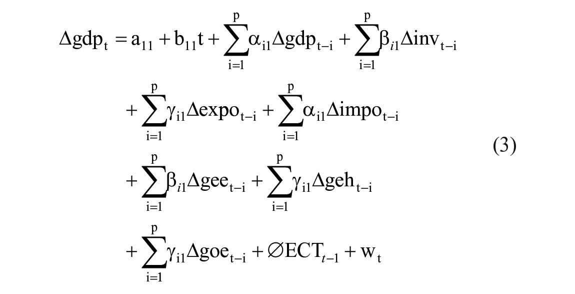
Where ECT is the Error correction term, $\varnothing$ adjustment coefficient, and ${\mathrm{w}}_{\mathrm{t}}$ error.

The Augmented Dickey-Fuller (ADF) Test: The general ADF model that is used for unit root test with both intercept and linear trend is specified as follows:

$$\Delta {\mathrm{y}}_{\mathrm{t}}={\alpha }_0+{\alpha }_1\mathrm{t}+\gamma \mathrm{y}+{\displaystyle \sum }_{\mathrm{i}=1}^{\mathrm{p}}{\beta }_i\Delta {\mathrm{y}}_{\mathrm{t}-\mathrm{i}}$$

$$H_0:\gamma =0$$

$$H_1:\gamma <0$$

and evaluated using the conventional t-ratio for γ:

$$t_{\gamma }=\frac{\widehat{\gamma }}{se\left(\widehat{\gamma }\right)}$$

Where $\widehat{\gamma }$ is the estimate of γ and se ( $\widehat{\gamma })$ is the standard error of the coefficient estimate.

The Phillips-Perron (PP) Test: Phillips and Perron (1988) advocated the use of a nonparametric unit root test to eliminate serial correlation. The PP approach calculates the non-augmented DF test equation after changing the coefficient’s t-ratio in order to avoid the effects of serial correlation on the asymptotic distribution of the test statistic. The PP method employs the following test statistic:

$${\tilde{t}}_{\gamma }=t_{\gamma }{\left(\frac{{\varnothing }_0}{f_0}\right)}^{1/2}-\frac{T(f_0-{\varnothing }_0)(se\left(\widehat{\gamma }\right))}{2{f_0}^{1/2}s}$$

where, $\widehat{\gamma }$ is the estimate of γ, $t_{\gamma }$ the t-ratio of $\gamma$ , $se\left(\widehat{\gamma }\right)$ the coefficient standard error, s the standard error of the test regression. ${\varnothing }_0$ is the consistent estimate of the error variance in the standard DF equation calculated as $\frac{\left(T-k\right)S^2}{T}$ , wherein k is the number of explanatory variable. Finally, $f_0$ is an estimator of the residual spectrum at zero frequency.

The Ng and Perron (NP) Test: Ng and Perron (2001) developed four test statistics, MZ_a, MZ_t, MSB, and MPT, using detrended GLS data, y_t^d. The test statistics are altered versions of Phillips and Perron’s, Z_a and Z_t statistics, Bhargava’s (1986) R₁ statistic, and the ERS Point Optimal Statistic.

Results and Discussion

Unit Root and Stationarity Test

To cross-check and thoroughly verify the correct sequence of integration for each series, we use the ADF, Phillips Perron, and Ng-Perron unit root tests, all of which assume that a series has a unit root under the null hypothesis. As per the ADF unit root test, the series gdp, inv, expo, impo, and goe all are I(1), while the remaining two series gee and geh both are I(0) (Table 2). The Phillips-Perron and Ng-Perron unit root tests yield identical and completely compatible answers with the ADF unit root test (Tables 3 and 4).

Table 2.

ADF Unit Root Test Results.

Variables	Level		First Difference		Inference
	Intercept	Intercept and trend	Intercept	Intercept and trend
gdp	−1.4412[0]	−2.8004[0]	−7.0170*[0]	−6.8969*[0]	I(1)
inv	−0.9146[0]	−2.0131[0]	−4.9720*[0]	−4.8889*[0]	I(1)
expo	−0.8779[0]	−2.1637[0]	−5.2298*[0]	−5.2056*[0]	I(1)
impo	−0.1802[0]	−1.6917[1]	−4.7207*[0]	−4.6008*[0]	I(1)
gee	−1.5071[0]	−4.5772*[0]	−10.2399*[0]	−10.0771*[0]	I(0) or I(I)
geh	−2.3460[0]	−5.7719*[0]	−9.3110*[0]	−9.1575*[0]	I(0) or I(1)
goe	−1.7118[0]	−2.0219[0]	−5.6579*[0]	−5.6231*[0]	I(1)

*

and ** denotes significance at the 1% and 5%levels. No. of lags selected by BIC is given in the square brackets.

Source. The authors.

Table 3.

PP Unit Root Test Results.

Variables	Level		First Difference		Inference
	Constant	Constant and trend	Constant	Constant and trend
gdp	−1.4751{2}	−2.8004{0}	−7.0170*{0}	−6.8969*{0}	I(1)
inv	−0.8943{4}	−2.1768{3}	−4.9244*{4}	−4.8324*{4}	I(1)
expo	−0.7687{6}	−2.1637{0}	−5.2949*{6}	−5.3573*{8}	I(1)
impo	−0.2730{2}	−2.0401{2}	−4.7207*{0}	−4.6008*{0}	I(1)
gee	−1.2105{2}	−4.7086*{3}	−11.8772*{4}	−12.4986*{5}	I(0) or I(1)
geh	−2.1193{3}	−5.9142*{5}	−28.9619*{31}	−28.9914*{31}	I(0) or I(1)
goe	−1.8197{1}	−2.0176{2}	−5.4076*{11}	−7.5929*{15}	I(1)

*

and ** denotes significance at the 1% and 5%levels. No. of bandwidth is given in the middle brackets.

Source. The authors.

Table 4.

Ng-Perron Unit Root Test Results.

Constant and trend
Variable	MZa	MZt	MSB	MPT
gdp	−7.32609(0)	−1.89697(0)	0.25893(0)	12.46720(0)	Non-Stationary
inv	−7.31915(0)	−1.86774(0)	0.25519(0)	12.52610(0)	Non-Stationary
expo	−7.78791(0)	−1.93432(0)	0.24837(0)	11.79370(0)	Non-Stationary
impo	−3.66704(0)	−1.33319(0)	0.36356(0)	24.51980(0)	Non-Stationary
gee	−15.67900***(0)	−2.79683***(0)	0.17838***(0)	5.83008***(0)	Stationary
geh	−16.44610***(0)	−2.86493***(0)	0.17420***(0)	5.55665***(0)	Stationary
goe	−6.54508(0)	−1.76175(0)	0.26917(0)	13.9305(0)	Non-Stationary
Constant only
Δgdp	−14.12700*(0)	−2.62983*(0)	0.18616**(0)	1.83979**(0)	Stationary
Δinv	−15.0244*(0)	−2.58318*(0)	0.17193*(0)	2.20690**(0)	Stationary
Δexpo	−14.7871*(0)	−2.65740*(0)	0.17971**(0)	1.88710**(0)	Stationary
Δimpo	−12.4346**(0)	−2.48934**(0)	0.20020**(0)	1.98618**(0)	Stationary
Δgee	−10.6242**(1)	−2.29609**(1)	0.21612**(1)	2.33987**(1)	Stationary
Δgeh	−12.6366**(0)	−2.5122**(0)	0.19880**(0)	1.94430**(0)	Stationary
Δgoe	−14.285*(0)	−2.66493*(0)	0.18655*(0)	1.74396*(0)	Stationary
Asymptotic critical values (Constant and trend)
1%	−23.80000	−3.42000	0.14300	4.03000
5%	−17.30000	−2.91000	0.16800	5.48000
10%	−14.20000	−2.62000	0.18500	6.67000
Asymptotic critical values (Constant only)
1%	−13.80000	−2.58000	0.17400	1.78000
5%	−8.10000	−1.98000	0.23300	3.17000
10%	−5.70000	−1.62000	0.27500	4.45000

*

, **, and *** denotes significance at the 1%, 5%, and 10% levels. No. of the lags selected by BIC is given in the small brackets.

Source. The authors.

We also applied the Zivot and Andrews (1992) unit root test allowing for one break. The test indicates a break in the dependent variable gdp in 1999. The Zivot-Andrews test allowing for one break indicates a break in year 1999, and it further establishes that the variables are still of mixed order of integration Table 5.

Table 5.

Zivot-Andrews Unit Root Test Results.

Variables in level	Type of break		Variables in the first diff.	Type of Break
	Intercept	Intercept and trend		Intercept	Intercept and trend
gdp	−3.544 [0]	−3.224 [0]	Δgdp	−8.212* [0]	−9.072* [0]
inv	−3.014 [0]	−3.000 [0]	Δinv	−5.489* [0]	−5.690* [0]
expo	−3.014 [0]	−3.495 [0]	Δexpo	−5.633* [0]	−5.463**[0]
impo	−3.503 [0]	−2.354 [0]	Δimpo	−5.554* [0]	−6.028* [0]
gee	−5.939* [0]	−6.369* [0]	Δgee	−10.485* [0]	−10.578* [0]
geh	−6.260* [0]	−6.916* [0]	Δgeh	−6.820* [1]	−6.973* [1]
goe	−4.501 [0]	−3.910 [0]	Δgoe	−6.102* [0]	−6.167* [0]

*

and ** denotes that the t-statistics are significant at the 1% and 5% levels, respectively. The value in the brackets is the optimum lag selected by the BCI criterion.

Source. The authors.

ARDL Bound Test of Cointegration

To apply ARDL modelling, each variable in the model must have an integration of the order of less than two. This precondition is met as the variables are either I(0) or I(1), and none are I(2). As a result, we proceed to apply the ARDL model to the variables gdp, inv, expo, impo, gee, geh, and goe with gdp as a dependent variable and the remaining as explanatory variables.

As a part of the second step of the ARDL approach, we conduct the bounds test on the dependent variable gdp, to determine whether the variables are cointegrated. The F-statistic value of 7.310093 rejects the null hypothesis of no level relationship at a 1% significance level since it exceeds the 1% I(1) critical bound value (Table 6). The bounds test results using the F-statistic reveals that cointegration exists between the variables with gdp as a dependent variable.

Table 6.

ARDL F-Bounds Test of Cointegration (Model: ARDL (2, 1, 1, 2, 1, 1, 1, 0).

Model type: Restricted constant and no trend
Null hypothesis: No level relationship
Test statistic	Value	Significance (%)	I(0)	I(1)
F-statistic	7.310093*	10.0	2.277	3.498
k	7	5.0	2.730	4.163
		1.0	3.864	5.694

*

Shows that the value is statistically significant at 1%.

Source. The authors.

Along with performing additional model adequacy checks, we estimate the ARDL (2, 1, 1, 2, 1, 1, 1, 0) ECM to verify the ARDL model’s validity when all co-integrated variables are included. The table below summarizes the results of the ECM. The error correct coefficient, ϕ in equation two, must be negative and highly significant to confirm a long-run equilibrium association among the variables while also allowing for the short-run adjustment dynamics to restore the long-run association in the event of a deviation from it.

The error-correction term coefficient (ETC) (−1) is −0.70317, which is expectedly negative and significant at 1% and has an absolute value very close to one. Thus, the ECM results validate the existence of a long-run relationship between variables while also demonstrating the short-run fast adjustment dynamics to equilibrium (Table 7).

Table 7.

Results of the ARDL Error Correction Regression.

Dependent Variable: Δ(gdp) (Model Type: Restricted Constant and No Trend)
Regressors	Coefficient	t-Statistic	Prob.
Δ(gdp(−1))	−0.35371	−5.48398*	0.0001
Δ(inv)	0.11755	1.79889	0.0922
Δ(expo)	0.03225	1.27658	0.2212
Δ(impo)	0.14134	2.83119**	0.0126
Δ(impo(−1))	0.15114	5.29772*	0.0001
Δ(gee)	0.24693	5.41437*	0.0001
Δ(geh)	−0.08791	−4.92028*	0.0002
Δ(goe)	0.03195	0.95199	0.3562
ECT(-1)	−0.70317	10.04387*	0.0000
R2 = 0.9030
Adjusted R2 = 0.8693
Durbin-Watson stat = 1.7895
Included observation = 32

*

and ** indicate level of significance at 1% and 5% respectively.

Source. The authors.

It makes sense to investigate the ARDL model’s adjustment equation’s speed. The large and negative ETC (−0.70317) implies that approximately 70.31% of total disequilibrium movements are corrected within a year. We hence, conclude that the coefficient is statistically significant at 1% based on the large value of the t-statistic (10.04387).

Table 8 summarizes the results of the long-run equilibrium relationships among the variables. The coefficients of variables inv, expo, and gee are positive and statistically significant at 1% and 5%. At the 5% level, the geh coefficient is negative and statistically significant, whereas the impo and goe coefficients are negative but not statistically significant. Thus, variables inv, expo, and gee have a long-run positive relationship with gdp, whereas impo, geh and goe have a long-run negative relationship with gdp (Table 8).

Table 8.

The Results of Levels Equation.

Dependent variable: gdp (Model Type: Restricted Constant and No Trend)
Regressors	Coefficient	t-statistic	Prob.
inv	0.48815	2.72788**	0.0156
expo	0.16203	2.16181**	0.0472
impo	−0.15141	−1.39108	0.1845
gee	0.77513	4.23948*	0.0007
geh	−0.26561	−2.79194**	0.0137
goe	−0.19642	−1.33919	0.2004
dum1999	−0.11371	−2.84059**	0.0124
c	2.02300	1.17797	0.2572
Included observation = 32

*

and ** denote the level of statistical significance at 1% and 5%, respectively.

Source. The authors.

The Diagnostic Checks of the ARDL Model

For the ARDL results to be valid and reliable, their errors must be normally distributed, homoscedastic uncorrelated. We verified this by performing the Jarque-Bera normality test on the residuals from the ARDL estimates. At a 5% level of significance, the Jarque-Bera test statistic is 1.1106, which does not reject the null hypothesis that errors are normally distributed (Table 9).

Table 9.

Results of the Diagnostic Test.

Type of test	Null hypothesis	Test Statistic	Value	df	Probability
Ramsey RESET (1) Test	The model is correctly specified	F-statistic	2.1022	(1, 14)	0.1691
Normality test	The residuals are normally distributed	Jarque-Bera	1.1106		0.5738
Breusch-Godfrey Serial Correlation LM Test	For up to ten lags, there is no serial correlation.	F-statistic	2.0019	F (10, 5)	0.2296
Breusch-Pagan-Godfrey Test of Heteroskedasticity	The residuals are homoscedastic	F-statistic	0.5849	Prob. F (15, 16)	0.8509
		Obs × R2	12.2954	Prob. Chi-Square. (16)	0.7234

Source. The authors.

The Breusch-Godfrey serial correlation test determines whether the residuals from the estimated model are serially uncorrelated. The p-value of the F-statistic (0.2296) does not rule out the null hypothesis of no serial correlation for up to ten lags. As a result, we accept that the residuals are serially uncorrelated (Table 9).

Similarly, we use the Breusch-Pagan-Godfrey test of heteroskedasticity to determine whether the residuals are heteroskedastic. The null hypothesis assumes homoscedastic residuals for this test. With an F-statistic of 0.5849 and a p-value of 0.8509, this test indicates that the null hypothesis is not rejected at 5%. As a result, the residuals are found to be homoscedastic. The F-statistic and likelihood ratio values for the specification test are insignificant statistically. As a result, the model’s specification is not incorrect (Table 9).

Additionally, we conducted the model stability test applying the CUSUM and CUSUM of square stability test. The cumulative sum of the recursive errors is used as the basis for the CUSUM test. This option generates a graph of the cumulative sum and the critical 5% lines. In case the cumulative sum crosses the area between the two critical lines, the test indicates parameter instability. The blue line graph never crosses the 5% significance line (Figure 1). As a result, the estimated model is determined to be stable. Similarly, the CUSUM of the square stability test indicates that the estimated model is stable because the blue line graph remains within the 5% significance line (Figure 2).

Figure 1.

CUSUM.

Figure 2.

CUSUM of Squares.

We then estimate the cointegrating relationship between the variables using FMOLS, DOLS, and canonical cointegrating regression (CCR) to assess the robustness of the ARDL model’s estimated long-run relationship. The FMOLS, DOLS and CCR estimators show the robustness of the long-run relationships. DOLS performs best among the three estimators, as revealed by its maximum value of R² (.9971), adj. R² (.9912) and minimum value of the standard error of regression 0.0295. The results of DOLS are also consistent with the long-run level relationships estimated by the ARDL approach (Table 10).

Table 10.

Results of Cointegrating Regression.

Variable	FMOLS		DOLS		CCR
	Coefficient	t-Statistic	Coefficient	t-Statistic	Coefficient	t-Statistic
inv	0.5181	6.6197* (0.0000)	0.4330	2.6136** (0.0259)	0.5163	4.6298* (0.0001)
expo	0.3098	10.6252* (0.0000)	0.2962	5.1832* (0.0004)	0.2875	7.5195* (0.0000)
impo	−0.3229	−5.8379* (0.0000)	−0.2781	−2.5513** (0.0288)	−0.3014	−4.2036* (0.0003)
gee	0.3669	5.4954* (0.0000)	0.4726	2.4783** (0.0326)	0.4398	3.3733* (0.0024)
geh	−0.0683	−2.4047** (0.0239)	−0.0417	−0.5188 (0.6151)	−0.0846	−1.5878 (0.1249)
goe	−0.0932	1.5805 (0.1266)	−0.7939	1.2493 (0.2336)	0.0126	0.1084 (0.9145)
dum1999	−0860	−3.4674* (0.0019)	−0.1497	−3.7748* (0.0036)	−0.1036	−3.0129* (0.0059)
c	−0.6586	0.7990 (0.4318)	−2.2531	−1.2792 (0.2297)	1.0640	0.9204 (0.3662)
	R2 = .9862		R2 = .9971		R2 = .9849
	Adjusted R2 = .9824		Adjusted R2 = .9912		Adjusted R2 = .9807
	S.E of Regression = 0.0429		S.E of Regression = .0295		S.E of Regression = .04495
	Jarque-Bera = 1.5243 (0.4666)		Jarque-Bera = 3.7355 (0.7410)		Jarque-Bera = 5.0357 (0.0806)

*

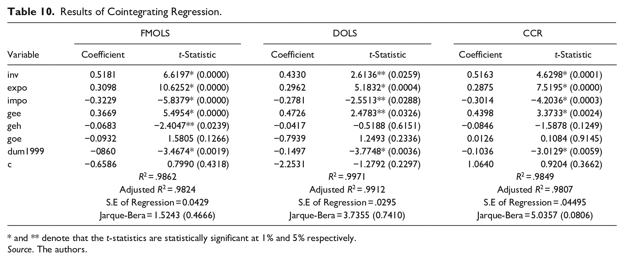
and ** denote that the t-statistics are statistically significant at 1% and 5% respectively.

Source. The authors.

The Toda Yamamoto Test of Causality

The Granger-causality test requires each variable to be stationary and also non-cointegrated. In the present case, the variables are cointegrated and exhibit a mixed integration order. In such a case, the Toda and Yamamoto (1995) causality test is preferred over the traditional Granger (1969) causality test as the former can be applied if the variables are cointegrated or included series are of mixed order of integration.

Following Toda and Yamamoto’s (1995) procedure, we selected the optimal lag p using optimal lag criteria and estimated an augmented VAR by adding lags to each variable equal to the maximum order of integration d_max in the set of variables. In the case of a VAR system involving two variables, Y and X, the Augmented VAR without any deterministic term is constructed as follows:

$$\begin{array}{l}{\mathrm{Y}}_{\mathrm{t}}={\alpha }_{11}+{\displaystyle \sum }_{\mathrm{i}=1}^{\mathrm{p}}{\alpha }_{\mathrm{i}1}{Y}_{t-i}+{\displaystyle \sum }_{\mathrm{i}=\mathrm{p}+1}^{\mathrm{p}+d_{max}}{\alpha }_{\mathrm{i}1}{\mathrm{Y}}_{\mathrm{t}-\mathrm{i}}\\ +{\displaystyle \sum }_{\mathrm{i}=1}^{\mathrm{p}}{\beta }_{\mathrm{i}1}{\mathrm{X}}_{\mathrm{t}-\mathrm{i}}+{\displaystyle \sum }_{\mathrm{i}=\mathrm{p}+1}^{\mathrm{p}+d_{max}}{\beta }_{\mathrm{i}1}{\mathrm{X}}_{\mathrm{t}-\mathrm{i}}+{\mathrm{u}}_{1\mathrm{t}}\end{array}$$

(4)

$$\begin{array}{l}{\mathrm{X}}_{\mathrm{t}}={\mathrm{a}}_{21}+{\displaystyle \sum }_{\mathrm{i}=1}^{\mathrm{p}}{\alpha }_{\mathrm{i}2}{\mathrm{X}}_{\mathrm{t}-\mathrm{i}}+{\displaystyle \sum }_{\mathrm{i}=\mathrm{p}+1}^{\mathrm{p}+d_{max}}{\alpha }_{\mathrm{i}2}{\mathrm{X}}_{\mathrm{t}-\mathrm{i}}\\ +{\displaystyle \sum }_{\mathrm{i}=1}^{\mathrm{p}}{\beta }_{\mathrm{i}2}{\mathrm{Y}}_{\mathrm{t}-\mathrm{i}}+{\displaystyle \sum }_{\mathrm{i}=\mathrm{p}+1}^{\mathrm{p}+d_{max}}{\beta }_{\mathrm{i}2}{\mathrm{Y}}_{\mathrm{t}-\mathrm{i}}+{\mathrm{u}}_{2\mathrm{t}}\end{array}$$

(5)

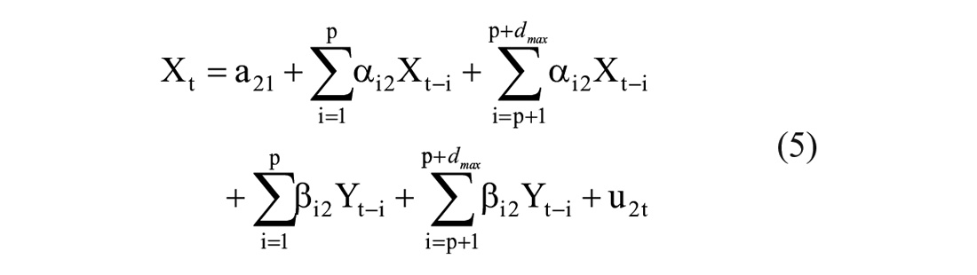
The modified Wald (MWald) test is applied on the above augmented VAR(p + d_max).

To test the causality running from variable Y to X, the null hypothesis is:

$${\mathrm{H}}_{\mathrm{0}}:{\beta }_{i1}=0,\mathrm{i}=1,2,\dots .\mathrm{p}.$$

To test the causality running from variable X to Y, the null hypothesis is:

$${\mathrm{H}}_0:{\beta }_{i2}=0,\mathrm{i}=1,2,\dots .\mathrm{p}.$$

Table 11 reports the results of the Toda and Yamamoto’s (1995) modified wald test of causality. We discovered no causal relationship between inv and gdp, feedback causality between expo and gdp, only one way causality from gdp to impo, feedback causality between gee and gdp, and also between geh and gdp, and no causal relationship between goe and gdp (Table 11).

Table 11.

Results of MWald Tests for Granger-causality [VAR(p + d_max) p = 3, dmax = 1)].

Null Hypothesis	Chi-sq	df	Prob.	Inference
inv does not Granger cause gdp	4.66367	3	0.1981	No Granger causality from inv to gdp
gdp does not Granger cause inv	5.390064	3	0.1454	No Granger causality from gdp to inv
expo does not Granger cause gdp	8.18876**	3	0.0423	Granger causality from expo to gdp
gdp does not Granger cause expo	15.13710*	3	0.0017	Granger causality from gdp to expo
impo does not Granger cause gdp	3.43413	3	0.3294	No Granger causality from impo to gdp
gdp does not Granger cause impo	44.06303*	3	0.0000	Granger causality from gdp to impo
gee does not Granger cause gdp	8.98686**	3	0.0295	Granger causality from gee to gdp
gdp does not Granger cause gee	9.120321**	3	0.0277	Granger causality from gdp to gee
geh does not Granger cause gdp	6.53873***	3	0.0881	Granger causality from geh to gdp
gdp does not Granger cause geh	122.9562*	3	0.0000	Granger causality from gdp to geh
goe does not Granger cause gdp	5.55994	3	0.1351	No Granger causality from goe to gdp
gdp does not Granger cause goe	1.463509	3	0.6907	No Granger causality from gdp to goe

*

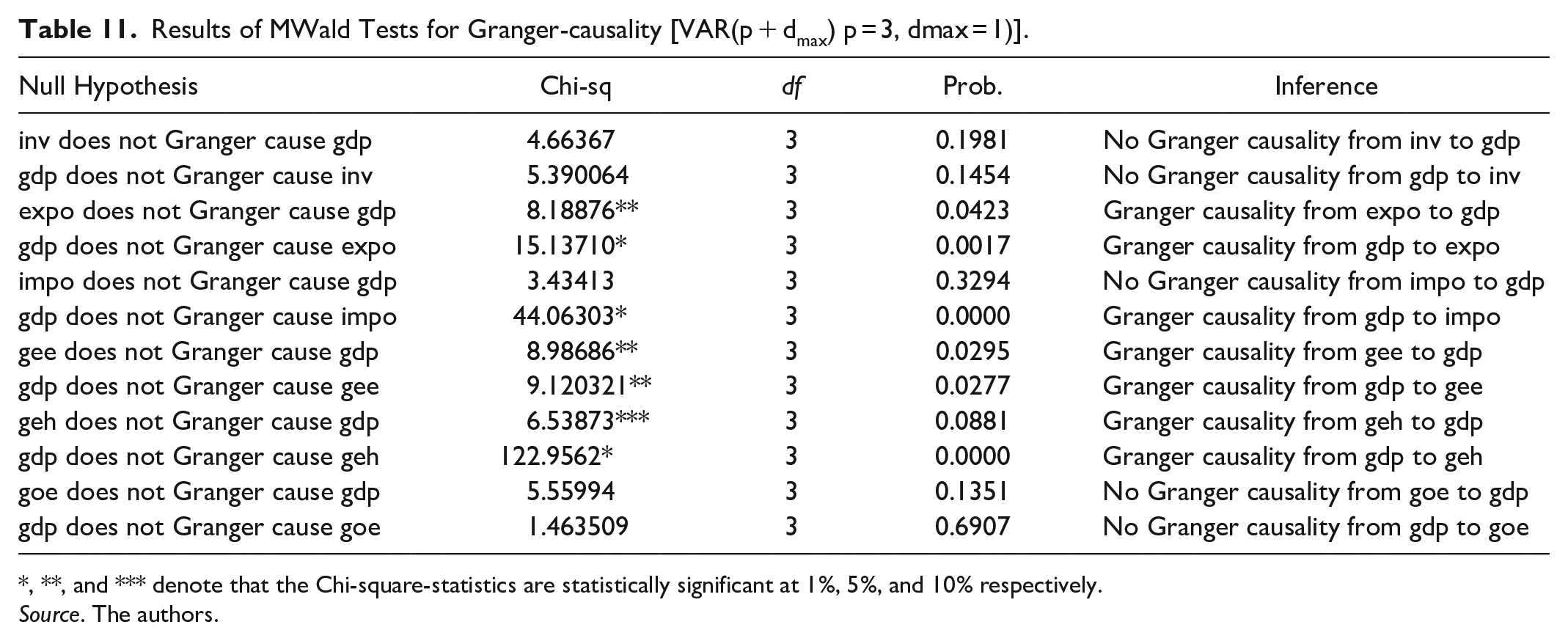
, **, and *** denote that the Chi-square-statistics are statistically significant at 1%, 5%, and 10% respectively.

Source. The authors.

The results of the cointegration test, the ARDL model, and three cointegrating regressions, FMOLS, DOLS, and CCR, demonstrate that investment, exports, and government education spending have a statistically significant and positive long-run effect on Saudi Arabia’s GDP growth. In comparison, imports have a statistically significant and negative impact on GDP growth in Saudi Arabia, while government spending on healthcare has a statistically insignificant and negative long-run effect on GDP growth.

The government of a country allocate its expenditures to various sectors considering the socio-economic requirements of that country. Economic growth is perhaps not a key determinant of government expenditure allocation to a sector. The government has different motives for allocating different types of government expenditures. Hence, labelling all government expenditures as either productive or equally productive is not reasonable. Some government expenditures might be productive, while others might be non-productive. Similarly, among the productive government expenditures, some expenditures might be more productive than others.

Several empirical studies have found evidence to support the positive contribution of government spending to economic growth (Christopher & De Utpal, 2020; Chu et al., 2020; Ebaidalla, 2013; Wu et al., 2010), while others (Onifade et al., 2020; Thabane & Lebina, 2016) have found evidence to the contrary. Most empirical evidence supports the view that government education spending contributes positively to a country’s economic growth (Islam, 2020a; Kutasi & Marton, 2020; Lingaraj et al., 2016; Mercan & Sezer, 2014). In contrast to most of the findings, Eggoh et al. (2015) demonstrated that public expenditures on education and health have a negative effect on economic growth.

Kutasi and Marton (2020) discovered that public spending on healthcare has a favorable effect on economic growth, whereas Eggoh et al. (2015) discovered that public expenditure on healthcare has a negative effect on economic growth. However, most of the research does not support the notion that government healthcare expenditure has a similar favorable influence on economic growth.

Our findings on the association of government education expenditures with GDP lend support to the findings of Mallick et al. (2016) and Alshahrani and Alsadiq (2014). However, our findings on the impact of government health expenditures on GDP growth differ from those of Alshahrani and Alsadiq (2014), who concluded that, in addition to public investment, public healthcare expenditures also spur economic growth in Saudi Arabia.

It is worth noting here that government other expenditures, the majority of which are non-productive type of expenditures, expectedly affect GDP growth negatively. The health sector in Saudi Arabia is overwhelmingly dependent on the foreign workforce and foreign health-related supplies, which could be the main reason why public health expenditures are not contributing to economic growth in Saudi Arabia.

Conclusion

We examined the long-run or equilibrium relationship and the short-run adjustment dynamics between variables GDP, investment, exports, imports, and three categories of government expenditures: education expenditure, health expenditure, and other government expenditures. Rather than treating different types of government expenditures equally and clubbing various government expenditures together, we include government expenditures on education, health, and the remainder of the government’s expenditures, referred to as other expenditures, as separate variables hypothesizing that they impact GDP growth differently. We analyzed the relationship among these variables using time series annual data on each variable from 1985 to 2018. Three distinct unit root tests were used to ascertain the order of integration for each variable. Additionally, we performed a unit root test with a structural break. We discovered that the included series were of integration with a mixed order. Consequently, the ARDL model, which is deemed fit, was used after an appropriate number of lags was selected using the automatic optimum lag selection method. The ARDL error correction model and bound test of cointegration established a long-run relationship between GDP, investment, exports, imports, and government expenditures on education, health, and other government spending. The analysis demonstrates that investment, exports and government education spending all have a long-run positive effect on GDP growth in Saudi Arabia. Against it, imports, government expenditures on healthcare and government other expenditures have a long-run negative effect on Saudi Arabia’s GDP growth. Toda and Yamamoto (1995) modified Wald tests of causality further corroborate causality from exports, government outlays on education, and government spending on health, to GDP growth. Hence, we infer from these findings that education expenditures stimulate economic growth while government health expenditures and government other expenditures retard economic growth in Saudi Arabia. Additionally, we infer that different categories of government expenditures have varying effects on GDP growth in Saudi Arabia. Therefore, prudent sectoral allocation of public expenditures is required to maximize the positive effects of the government budget on GDP and stimulate economic growth in Saudi Arabia.

Moreover, these findings have policy implications for the government while allocating its total expenditures. Allocating more expenditures to education and cutting down inessential spending on healthcare and government other non-productive expenditures will enhance economic growth in Saudi Arabia. Alternatively, reduced ownership and management by the government and increased participation of the private sector in the ownership and management of healthcare can improve the efficiency of resources used in the healthcare sector and eventually boost economic growth as envisaged in the Saudi Vision 2030 (Vision, 2030), which also underlines the role of the private sector as the main engine for socio-economic reforms for transforming the Saudi economy toward income diversification and growth with improved competitiveness.

Lastly, we are aware that the empirical research based on time series data require a few more observations than we had which is a limitation of this study. The future research can further broaden this study by including all category of the public expenditures as explanatory variables.