
Abstract
We examine the hedging/safe-haven ability of gold, the US dollar, bonds, crude oil, and Bitcoin against stocks using the unconditional quantile regression (UQR). We reveal that hedging (safe-haven) effect generally decreases (increases) with the quantiles of asset returns and find an asymmetric flight from stocks to the US dollar as well as asymmetric stock-gold, stock-bond, and stock-oil contagion. Finally, we find a connection between the asymmetric safe haven and asymmetric cross-asset flights/contagion. Therefore, investors seeking hedging and safe-haven assets and investigating flights or contagion should consider the feature of extremes of assets returns.
Keywords
Highlights
A quantile-based unconditional quantile regression is applied to gold, the USD, bonds, oil and Bitcoin.
Hedging (safe-haven) effects decrease (increase) with the quantile of asset returns.
Asymmetric flight-to-USD and stock-gold, stock-bond and stock-oil contagion is found.
The UQR estimations show that the USD can be the most effective safe-haven asset during the crisis period.
OLS misevaluates the hedging, safe-haven at the extremes of the return distribution.
Introduction
Recently, analyses of hedging/safe-haven assets have focused mainly on the global financial crisis (GFC) of 2008, which caused traders and investors to seek safe-haven assets against other financial instruments. Investigation of hedging/safe-haven assets has attracted much attention over the last decade (e.g., see Baur & Lucey, 2010; Baur & McDermott, 2010, and references therein). In these studies, the term “weak hedges” refers to assets whose returns under normal conditions are not related to other assets being hedged, while strong hedges are those whose returns are negatively correlated with those other assets during normal (non-stressed) conditions. In contrast, weak (strong) safe-haven assets refer to assets whose returns are uncorrelated (negatively correlated) with other assets during periods of financial stress.
In addition to looking for hedges and/or safe havens assets, investors want to understand the impact of a flight-to-quality and contagion effects during periods of market stress. For example, Forbes and Rigobon (2002) study the cross-country stock market contagion, and Dungey et al. (2006) analyze contagion among bond markets. Gulko (2002) and Baur and Lucey (2009) analyze the contagion effect between stocks and bonds, while, Gulko (2002), de Goeij and Marquering (2004), Connolly et al. (2005), Bansal et al. (2009) analyze the flight from stocks to bonds. Goyenko and Sarkissian (2010) define a flight to liquidity in terms of illiquidity in short-term U.S. Treasuries, and Chang et al. (2021) linked gold’s safe-haven status to a flight-to-quality property based on gold’s volatility regime.
Methodologies used to empirically assess hedging and safe-haven relationships as well as flight-to-quality and contagion effects have evolved in different strands of the literature, including the parametric model strand (Baur & Lucey, 2009, 2010; Baur & McDermott, 2010; Bekaert et al., 2014; Dungey et al., 2020), the nonparametric model strand (Bouri et al., 2017; Candelon & Tokpavi, 2016; Mensi et al., 2016) and the tail dependence strand (Apergis et al., 2020; Fry-McKibbin et al., 2019; C. S. Liu et al., 2016; Reboredo, 2013). Among these approaches, the parameter-regression estimation approach is the most popular as it is simple to implement and the resulting estimates (e.g., beta coefficients) can be readily interpreted. In contrast, parametric approaches such as ordinary least squared (OLS) techniques that use conditional mean estimators only characterize the mean of the relationship between the alternative asset and the reference asset. Given investor heterogeneity, a conditional mean estimation may under- or over-estimate cross-asset linkage (e.g., hedging, safe-haven, flights and contagion effects), leading to misdirected trading and investing.
A few studies note that conditional mean estimators do not describe the hedging, safe-haven, flights and contagion roles of conventional safe assets particularly well. For example, Hussain Shahzad et al. (2017) use a quantile-on-quantile approach to estimate the relationship between quantiles of gold (bonds) and those of stock markets. They find that gold serves as a strong hedge for stock portfolios, except when both markets are under stress, and that investors move capitals from equities to benchmark bonds when both are in lower quantiles. Baur and Kuck (2020) explore gold’s safe-haven ability against U.S. stock markets, finding that the strongest safe-haven effects occur in the upper quantiles when gold has large positive returns, and that investors flee from stocks to gold when stocks show extreme negative returns. In contrast, Hussain Shahzad et al. (2017) examine gold’s safe-haven property for stock and bond markets of G-7 countries and find that gold does not act as a safe haven for those markets. Hasan et al. (2022) use a quantile regression, and a quantile-on-quantile regression with data from December 30, 2013, to February 21, 2021 and show that Bitcoin, the US dollar, and crude oil (WTI) have no safe-haven properties with respect to cryptocurrency policy uncertainty (UCRY Policy) index. Assifuah-Nunoo et al. (2022) re-examine crude oil-stock market co-movement in the context of oil-exporting countries in Africa using the quantile regression approach and find that crude oil does not act as safe-haven instrument against stock markets volatility. Gupta and Sharma (2023) examine the hedging and safe-haven properties of global listed infrastructure sector indices versus stocks and bonds and find that infrastructure investing is neither a hedge nor a safe-haven. Mensi et al. (2022) use the quantile coherency method to examine the quantile dependence between precious metals and foreign exchange markets and show that gold is a good safe-haven asset against currencies. Kumar and Padakandla (2022) test the safe-haven properties of Bitcoin and gold using Wavelet quantile correlation and show that gold is a better safe-haven instrument than Bitcoin. However, these studies mostly address a given asset’s hedging (safe-haven) properties across all parts of its return distribution. Few study investigate flights or contagion in the same manner.
We investigate the hedging/safe-haven properties of gold, the USD, 10-year government bonds, crude oil and Bitcoin for stock markets in the U.S., Canada, Germany, and Japan using an unconditional quantile regression model. As our sample period, which spans from January 2002 to December 2021, covers episodes of sustained uncertainty (e.g., the GFC and the subperiod of COVID-19), we also analyze flights/contagion by comparing the dependence between stocks and considered assets during that crisis period to the benchmark period. In contrast to most previous empirical studies, our study (1) provides a detailed analysis of the short-term hedging/safe-haven analysis of the considered assets against stocks across the entire return distribution, (2) assesses whether OLS under- or overestimates the hedging (safe-haven) abilities of the considered assets given investor heterogeneity, and (3) investigates whether flight-to-quality and contagion behave differently under extreme market conditions, and explains the asymmetric relationship between each considered asset and the stock market using investor behavior.
Our study is similar to other studies that also examine the hedge and safe-haven properties of gold, bonds and crude oil. However, our study extends this literature by providing a more complete picture of hedging/safe-haven properties of gold, the USD, bonds, crude oil, and Bitcoin across the return distribution. Moreover, previous studies do not investigate flights and contagion properties at all parts of the return distribution. By addressing these issues, our study fills gaps in, and makes unique contributions to the existing literature.
Specifically, our study contributes to the literature by investigating the asymmetric relationships between various asset and the stock market, and their asymmetric flight-to-quality and contagion effects. In contrast to previous studies, we use an unconditional quantile regression (UQR) approach to obtain a more complete picture of hedging/safe-haven properties of each considered asset across the return distribution, and to help identify whether asymmetric flights and contagion occur under market stress. We then use investor behavior to explain asymmetric hedging and safe-haven effects.
In summary, our study reveals the following: first, consistent with several extant studies in the literature (e.g., Baur & Lucey, 2010; Baur & McDermott, 2010; Ciner et al., 2013), the results of our UQR estimation indicate that gold and crude oil provided strong hedging effects against stocks in the U.S. and Germany during the pre-GFC period. Nevertheless, this hedging ability weakened after the GFC, perhaps due to post-crisis homogeneity in stock-gold and stock-oil correlations (Baruník et al., 2016; Junttila et al., 2018). Hedging effectiveness for the USD increased after the GFC for all countries, indicating that the relationship between the USD and stocks strengthened after that crisis period (Tachibana, 2018). Bitcoin offered strong hedging effects against stocks in the U.S. and Canada after the GFC (Bouri et al., 2017; Kang et al., 2019).
The OLS method confirms that in the post-GFC period, gold was a strong hedging asset for the U.S., and the UQR estimation shows the same results when gold’s return distribution is below a fairly low quantile of 0.3. Although its strong hedging ability was confirmed by both the OLS and UQR estimations, gold did not offer investors risk-reducing portfolio diversification in the U.S. market after the financial crisis because its hedging ability occurs when the gold occurs at a gold market is bearish (Hussain Shahzad et al., 2017). This finding illustrates that employing a traditional OLS method and then confirming gold as a hedging asset for the U.S. stock markets post-GFC can produce a misguided suggestion to risk management.
Second, our UQR estimation shows that gold, the USD, bonds and Bitcoin returns act as weak safe havens against stocks returns for all countries over all periods when the returns of these assets exceed specific thresholds (W. Liu, 2020). For example, gold serves as a weak safe-haven beyond the low quantile (0.1) for both the U.S and Germany, and in the upper quantile (0.8) for Canada and Japan before the GFC. We also find that the safe-haven ability offered by gold, bonds and crude oil weakened during the GFC, which may have been caused by bidirectional interdependence with stocks (Choudhry et al., 2015). In addition, the UQR estimations suggest that the USD’s safe-haven ability strengthened during the GFC, and that the USD is the most valid safe haven. These two findings may be explained by the USD’s appreciation in the second half of 2008 (Fratzscher, 2009; McCauley & McGuire, 2009).
The safe-haven effect of crude oil against stocks is confirmed for the U.S, Canada and Germany at the upper quantile of oil returns prior to the GFC; however, this effect is greatly diminished after the GFC. This result can be explained by observing that stock-oil linkage became significantly stronger during the GFC (see Creti et al., 2013; Filis et al., 2011; Kolodziej et al., 2014). Consistent with Baur et al. (2018) and Kang et al. (2019), Bitcoin provided a weak safe-haven ability against stocks for all countries during the post-crisis period when its returns were higher than the median quantile.
Third, hedging/safe-haven effects for the assets studied respond differently and in highly asymmetric patterns. The UQR approach shows the hedging effect of each asset is more pronounced at the lower end of the asset’s returns and is underestimated by OLS. In contrast, UQR shows the safe-haven effect is more pronounced at the upper end of the asset’s return distribution and is overestimated by OLS. The hedging effect of each asset decreases with the quantiles of its return distribution, while the safe-haven effect increases. This finding implies that the hedging effect of each asset is maximized at the lowermost quantiles and minimized at the uppermost quantiles, and vice-versa for the safe-haven effect. Baur and Kuck (2020) also find the safe-haven ability of gold increases with gold returns. Owing to these asymmetric patterns, our UQR framework reveals a change in the dispersion of the unconditional asset returns distribution, a phenomenon underlying the conditional mean estimation.
Fourth, our study finds stock-gold, stock-bond and stock-oil contagion when the returns of these assets are below the median quantile, which may be due to investor behavior (Kumar & Persaud, 2002). In contrast, a flight is identified from stocks to the USD for all countries with different country-specific thresholds of USD returns. A possible reason for this finding may be flight-to-safety (Baele et al., 2020). Furthermore, an asymmetric contagion between a haven asset and stocks exists if the safe-haven ability of the asset was weaker during the GFC period than in other times. In contrast, if the safe-haven ability of an asset was stronger during the crisis period than in non-crisis periods, an asymmetric flight from stocks to this asset is observed.
Finally, our results suggest that investor behaviors could explain the asymmetry hedging/safe-haven behaviors of these assets. On the one hand, the hedging ability of these assets is generally maximized at the lowest quantile of the return distribution, which can be explained by the representativeness heuristic (Grether, 1980). As the returns of hedging assets increase, investors may become more focused on pursuing the returns and overlook the original function (i.e., hedging) of these assets. This change in investor behavior may affect the price and volatility of hedging assets, further reducing their hedging ability. Conversely, as the returns of safe-haven assets increase more investors may be attracted to them. This increased demand could strengthen the asset’s role as a safe haven as more investors seek out the asset, which can help minimize the losses during times of market stress. Investors’ loss aversion may be associated with the safe-haven role of these assets in the highest quantile (Baur & McDermott, 2016; Kahneman & Tversky, 1979; Tversky & Kahneman, 1991).
The remainder of the paper is structured as follows. Section 2 presents the methodology. Sections 3 and 4 discuss the data and present the empirical results. Conclusions are provided in Section 5.
Econometric Model
Unconditional Quantile Regression
OLS has been a standard instrument for conducting hedging (safe-haven) analyses in empirical finance studies (Baur & Lucey, 2010; Baur & McDermott, 2010). It shows how the conditional expected returns of a safe haven respond to changes in stock returns, ceteris paribus. However, conventional OLS regression is not well-suited to explain the distribution of a variable, especially when a variable contains asymmetric and (or) heavy tailed data, such as asset returns. As Shefrin (2008) and others have suggested, investor heterogeneity often results in a skewed and fat-tailed distribution of stock returns. Heterogeneity of investors is crucial to the analysis of dependence between the returns of an asset and those of stocks. A regression method that is robust to heterogeneity should therefore be used. OLS only considers changes in the means. Therefore, may under- or over-estimate dependent response variables with heterogeneous distributions, see Koenker and Hallock (2001) and Koenker (2005). Koenker and Bassett (1978) proposed a conditional quantile regression method (CQR) to model the relation between independent variables and specific quantiles of the dependent variable. Koenker and Hallock (2001) pointed out that CQR could minimize estimation bias of skewed samples.
Although CQR is a heterogeneity-consistent method, its implications are not always fully recognized, giving rise to misleading interpretations of CQR results. To address this problem, researchers have resorted to using the UQR method (Firpo et al., 2009). The UQR approach has some important advantages over the CQR model. For example, UQR can gage the whole impact of participation in direct marketing on gold purchase at specific quantiles in the gold-return distribution. Moreover, UQR estimates provide a means to isolate specific parameter effects that are covered by the conditional effects. A gentle introduction and clarifying application can be found in Borah and Basu (2013). This new approach studies the direct effects of covariates on unconditional (marginal) distributions of the dependent variable by using a recentered influence function (RIF)-OLS regression. Let Y denote the explained variable with distribution function

Firpo et al. (2009) call the conditional expectation of the
The Empirical UQR Model
This paper augments the OLS model by modeling the relation between the considered assets (gold, the USD, bonds, crude oil, and Bitcoin) and stocks using the UQR to investigate how normal and extreme negative stock returns vary across different quantiles of asset returns. Before defining the UQR model for the safe haven analysis, we first specify the standard OLS model as our benchmark model, following Baur and McDermott (2010) and Baur and Lucey (2010).
The standard OLS model, assessing the hedging (safe haven) ability of considered asset against the stock market, takes the form of

where
Our study extends the unconditional quantile regression model to account for the hedging (safe-haven) effects by adding regressors containing

The structure of the model assumes that the stock returns can affect the return of considered assets; this assumption is consistent with the safe haven hypothesis. If stocks exhibit extreme negative returns, investors would buy safe havens and bid up their prices. In practice, the estimation procedure can be divided into two steps. The first step is to estimate the RIF of the
The previous discussion leads us to the following testable hypotheses.
Hypothesis 1A: Gold is at least a weak hedge for the stock market.
Hypothesis 1B: The USD is at least a weak hedge for the stock market.
Hypothesis 1C: Bonds are at least a weak hedge for the stock market.
Hypothesis 1D: Crude oil is at least a weak hedge for the stock market. Hypothesis 1E: Bitcoin is at least a weak hedge for the stock market.
If Hypothesis 1A, 1B, 1C, 1D, or 1E holds, investors holding gold, the USD, bonds, crude oil or Bitcoin reduce the risk of adverse price movements in the stock market during normal times. Following the definition suggested by the existing literature, we assume that the asset offers a weak or strong hedging effect for both stocks in the OLS estimation if
Hypothesis 2: The hedging ability of considered assets against stocks is pronounced in the extreme market conditions.
If Hypothesis 2 holds, the considered asset’s hedging effect would be of larger economic and statistical significance at the uppermost (0.95) and/or lowest (0.05) quantiles of its return distribution than at median quantiles.
Hypothesis 3A: Gold provides at least a weak safe-haven ability against the stock market.
Hypothesis 3B: The USD provides at least a weak safe-haven ability against the stock market.
Hypothesis 3C: Bonds provide at least a weak safe-haven ability against the stock market.
Hypothesis 3D: Crude oil provides at least a weak safe-haven ability against the stock market.
Hypothesis 3E: Bitcoin provides at least a weak safe-haven ability against the stock market.
If Hypothesis 3A, 3B, 3C, 3D, or 3E holds, investors holding gold, the USD, bonds, crude oil or Bitcoin retain or even gain values during periods of economic downturn. For the OLS model, an asset serves as a weak safe haven when
Hypothesis 4: The safe-haven capacity of considered assets against stocks is pronounced in the extreme market conditions.
If Hypothesis 4 holds, the asset’s safe-haven effect would be of larger economic and statistical significance at uppermost (0.95) and/or lowest (0.05) quantiles of its return distribution than at the median quantiles.
Hypothesis 5: Hedging and safe-haven effects of these assets are asymmetric, and heterogeneity causes investors to respond differently to normal and extreme stock market conditions across the return distributions.
If Hypothesis 5 holds, the pessimistic investors respond asymmetrically to normal and extreme market conditions in comparison to the optimistic investors. Hence, the asymmetric hedging effect should be distinctly different from the asymmetric safe-haven effect in the lower (upper) quantiles of the asset return distribution than in the median parts.
Moreover, the asymmetric safe-haven pattern indicates that the asset may or may not perform safe-haven role at some extreme quantile of returns, implying that the flights or contagion could be asymmetric. For example, suppose an asset provides a safe-haven protection against stocks across all quantiles before the GFC but the safe-haven ability existed only at high quantile of asset returns after the GFC, then a contagion between this asset and stocks will occur at low quantiles of asset returns. This inference leads to Hypothesis 6.
Hypothesis 6: Flights or contagion effects of these assets are asymmetric across quantiles.
Baur and Lucey (2009) argued that a flight from stocks to an asset is identified if
Data
Daily data on stock market indices, nominal exchange rates, and the spot prices of gold and crude oil are collected between January 5, 2002 and December 31, 2021 from Datastream. We collected Bitcoin price denominated in USD for the period from January 5, 2014 to December 31, 2021 from www.coindesk.com, which aggregates prices from selected exchanges into a reference price series. Note that we collected Bitcoin prices after 2014 given the December 2013 crash in that market. The stock indices used are the U.S. S&P500 composite index, Canada S&P/TSX composite index, Germany DAX composite index and Japan Nikkei 220 index. Nominal exchange rates are defined as the number of units of a domestic currency per unit of USD. We consider the Broad Trade-Weighted Exchange Index (TWEXB) for the U.S., Canadian dollar (CAD) for Canada, Euro for Germany and Japanese Yen for Japan. The crude oil price used in the study is the West Texas Intermediate (WTI) spot crude oil price. The price of gold is measured in USD per ounce.
The return series
Table 1 presents descriptive statistics for daily stock, bond, exchange rate, gold, crude oil and Bitcoin returns. The average of returns (in absolute values) are smaller than their standard deviations, indicating relatively high volatilities. Most of the returns series are highly leptokurtic, suggesting that the normality assumptions for return distribution are violated. It can be observed that during the crisis period the data distributions exhibit higher kurtosis than during the pre-crisis period, suggesting a larger probability of extreme market conditions (good or bad) during the crisis period. Similarly, different levels of kurtosis are seen during the COVID-19 period compared to other periods. This indicates that the whole samples should be divided into four subsamples (pre-crisis, crisis, post-crisis and COVID-19) to investigate the hedging/safe-haven effects.
Descriptive statistics of gold, stock and exchange rate return series.
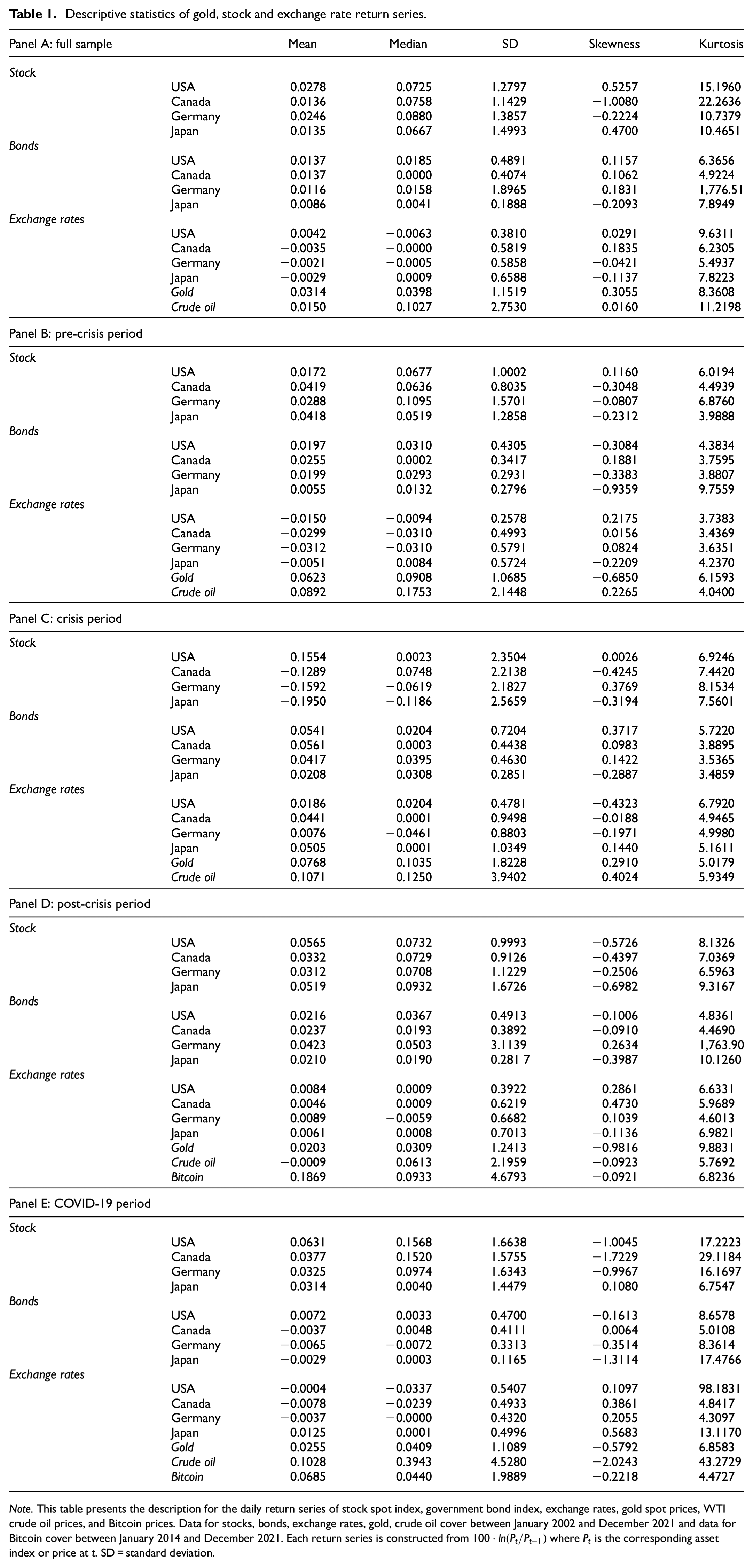
Note. This table presents the description for the daily return series of stock spot index, government bond index, exchange rates, gold spot prices, WTI crude oil prices, and Bitcoin prices. Data for stocks, bonds, exchange rates, gold, crude oil cover between January 2002 and December 2021 and data for Bitcoin cover between January 2014 and December 2021. Each return series is constructed from
Empirical Analysis
Results of UQR Estimation
The analysis begins with estimates from the OLS model as the benchmark and the UQR as the alternative approach. In the UQR model, 19 estimates for
Estimation results of UQR model for gold.

Note. This table presents the estimation results from mean regression (OLS) and unconditional quantile regression (UQR) for the daily return series of gold prices and stock index for the U.S., Canada, Germany and Japan. The estimation results over the pre-crisis, crisis, post-crisis and COVID-19 periods are reported in each panel. The estimates of
Estimation results of UQR model for USD.

Note. This table presents the estimation results from mean regression (OLS) and unconditional quantile regression (UQR) for the daily return series of exchange rate and stock index for the U.S., Canada, Germany and Japan. The estimation results over the pre-crisis, crisis, post-crisis and COVID-19 periods are reported in each panel. The estimates of
Estimation results of UQR model for bonds.

Note. This table presents the estimation results from mean regression (OLS) and unconditional quantile regression (UQR) for the daily return series of government bond index and stock index for the U.S., Canada, Germany, and Japan. The estimation results over the pre-crisis, crisis, post-crisis and COVID-19 periods are reported in each panel. The estimates of
Estimation results of UQR model for crude oil.

Note. This table presents the estimation results from mean regression (OLS) and unconditional quantile regression (UQR) for the daily return series of crude oil prices and stock index for the U.S., Canada, Germany, and Japan. The estimation results over the pre-crisis, crisis, post-crisis, and COVID-19 periods are reported in each panel. The estimates of
Estimation results of UQR model for Bitcoin.
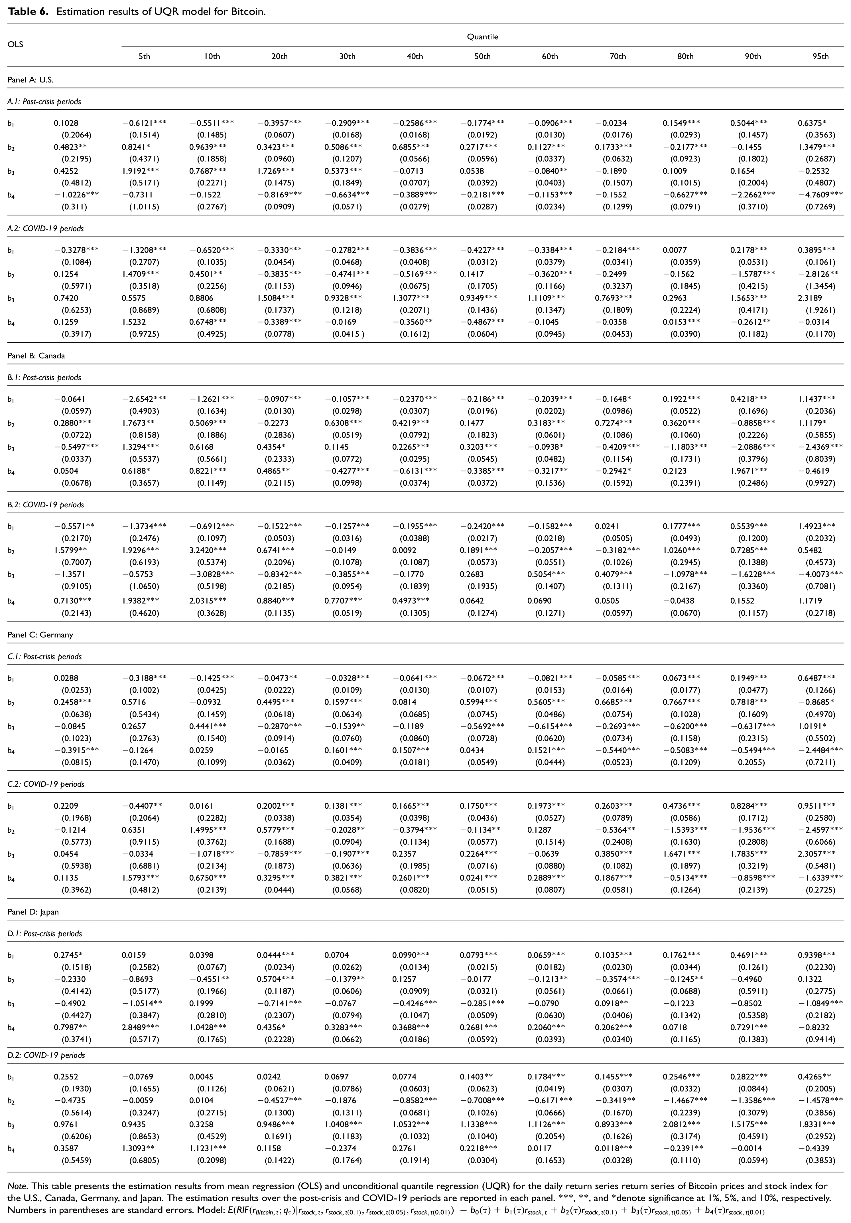
Note. This table presents the estimation results from mean regression (OLS) and unconditional quantile regression (UQR) for the daily return series return series of Bitcoin prices and stock index for the U.S., Canada, Germany, and Japan. The estimation results over the post-crisis and COVID-19 periods are reported in each panel. ***, **, and *denote significance at 1%, 5%, and 10%, respectively. Numbers in parentheses are standard errors. Model:
Generally, most of the UQR estimates of
We also note that the estimates of
The results of UQR estimation indicate that the estimates of
Moreover, estimates of
Results of Hedging Analysis
Figures 1 to 5 present the OLS and UQR estimates of hedging effects for gold, the USD, bonds, crude oil and Bitcoin. The hedging assets’ responses to stock returns are plotted in the upper-left, upper-right, lower-left and lower-right subplots for the pre-crisis, crisis, post-crisis and COVID-19 periods, respectively (we report hedging effects based on the full sample in Figure A.1 in the Appendix). In each plot, the x-axis indicates quantile scale, and the y-axis indicates the hedges, using the estimates of
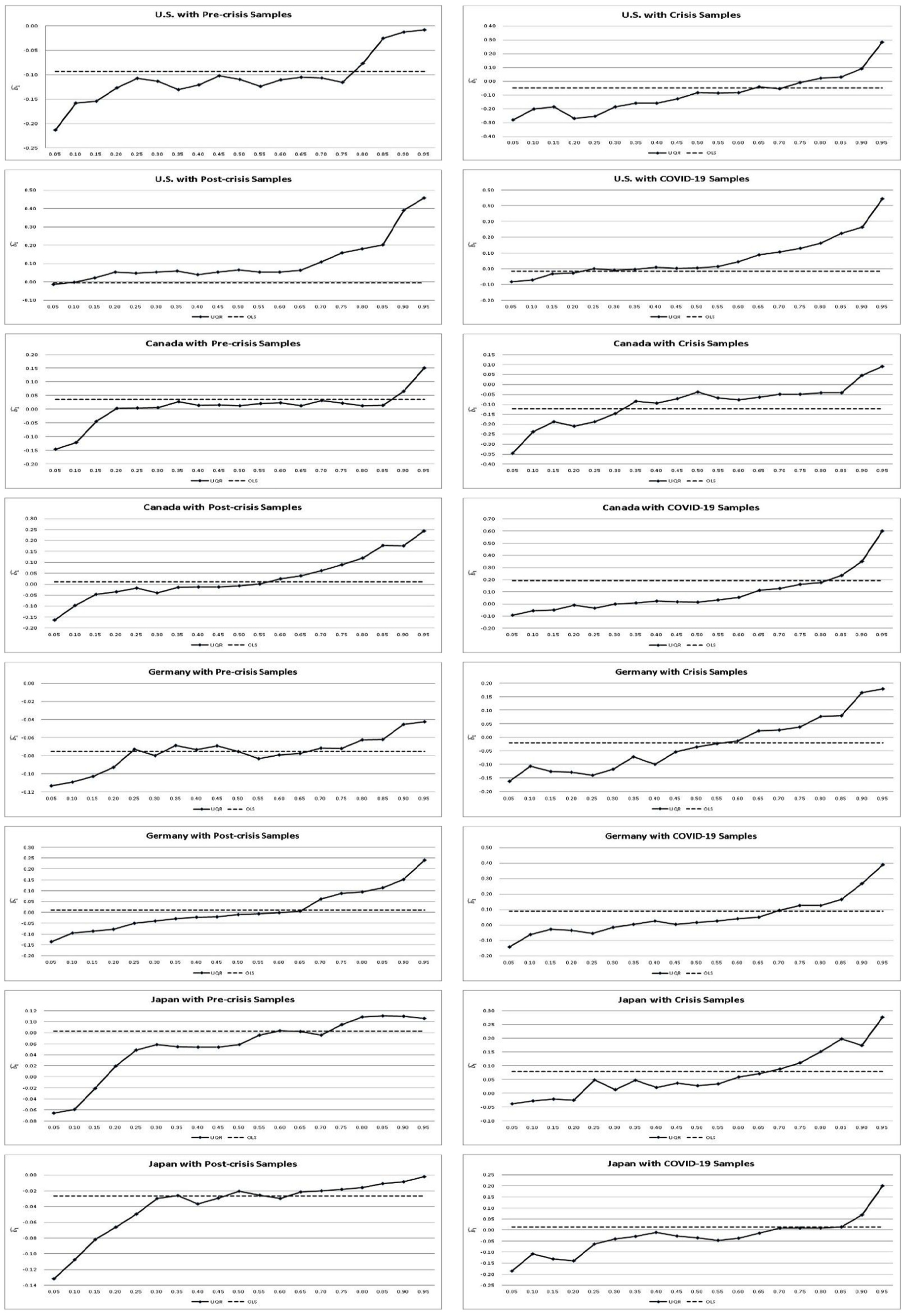
Hedging effect of gold of UQR estimates (solid lines) versus OLS estimates (dotted lines) across quantiles. Over all subperiods, the estimates of b1 generally increase with the quantiles of return distribution of gold, supporting that the hedging effect is asymmetric and is maximized at around the lowermost quantiles (0.05–0.1).

Hedging effect of USD of UQR estimates (solid lines) versus OLS estimates (dotted lines) across quantiles. Over all subperiods, the estimates of b1 generally increase with the quantiles of return distribution of USD, supporting that the hedging effect is asymmetric and is maximized at around the lowermost quantiles (0.05–0.1).

Hedging effect of bonds of UQR estimates (solid lines) versus OLS estimates (dotted lines) across quantiles. Over all subperiods, the estimates of b1 generally increase with the quantiles of return distribution of bonds, supporting that the hedging effect is asymmetric and is maximized at around the lowermost quantiles (0.05–0.1).

Hedging effect of crude oil of UQR estimates (solid lines) versus OLS estimates (dotted lines) across quantiles. Over all subperiods, the estimates of b1 generally increase with the quantiles of return distribution of crude oil, supporting that the hedging effect is asymmetric and is maximized at around the lowermost quantiles (0.05–0.1).
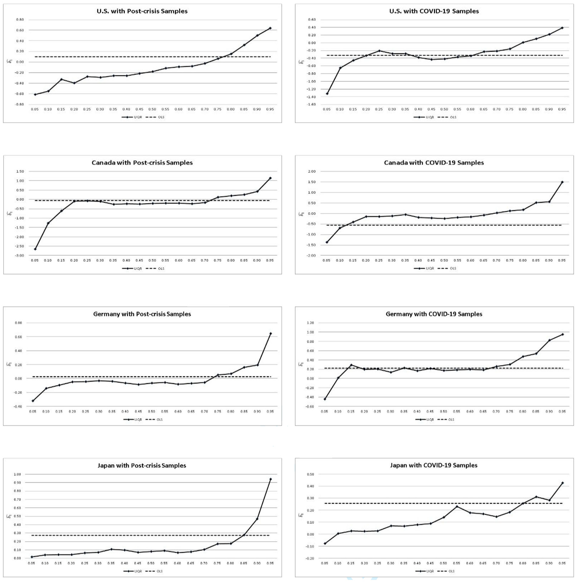
Hedging effect of Bitcoin of UQR estimates (solid lines) versus OLS estimates (dotted lines) across quantiles. Over all subperiods, the estimates of b1 generally increase with the quantiles of return distribution of Bitcoin, supporting that the hedging effect is asymmetric and is maximized at around the lowermost quantiles (0.05–0.1).
Results from the UQR approach show strong hedging effects for gold and bonds for all of the countries analyzed over all subperiods, confirming Hypotheses 1A, 1C, and 2. However, hedge effects were more robust prior to the GFC compared to the post-crisis period in the U.S. and Germany, which may be explained by the pronounced homogeneity in stock-gold and stock-bond correlations post-GFC (Baruník et al., 2016).
Consistent with the OLS estimation, the UQR estimations show that the hedging effect of the USD is stronger in the post-crisis period than the pre-crisis period. This finding supports Hypothesis 1B and 2.
Crude oil is shown to have a hedge effect for stock markets in the U.S., Germany and Japan before the GFC. This finding, supporting Hypothesis 1D and 2, indicates that, the correlation between crude oil returns and stock returns after the GFC has been higher than it was before the crisis. A possible explanation is that the stock-oil linkages increase during crisis periods because investors react to crises by increasing their positions in crude oil and then enhance the connection between the crude oil and stocks (Junttila et al., 2018).
Finally, Bitcoin shows a strong hedging effect against stocks in the U.S., Canada and Germany after the GFC (Bouri et al., 2017), supporting Hypothesis 1E and 2. Due to its highly volatile prices, Bitcoin attracts more speculative and short-term trading activity. Therefore, the hedging effect could occur when traders use Bitcoin to hedge stocks.
Results of Safe-Haven Analysis
Figures 6 to 10 reveal estimates of the safe-haven effect of gold, the USD, bonds, crude oil and Bitcoin against stocks. The safe-haven responses to stock returns are plotted in the upper-left, upper-right, lower-left and lower-right subplots for the pre-crisis, crisis, post-crisis and COVID-19 periods, respectively. The safe-haven effects based on the full samples are presented in Figure A.2 in the Appendix. Consistent with Choudhry et al. (2015), the OLS estimation shows that gold, the USD and bonds are weak safe havens for stock investors in all countries over the post-crisis periods.
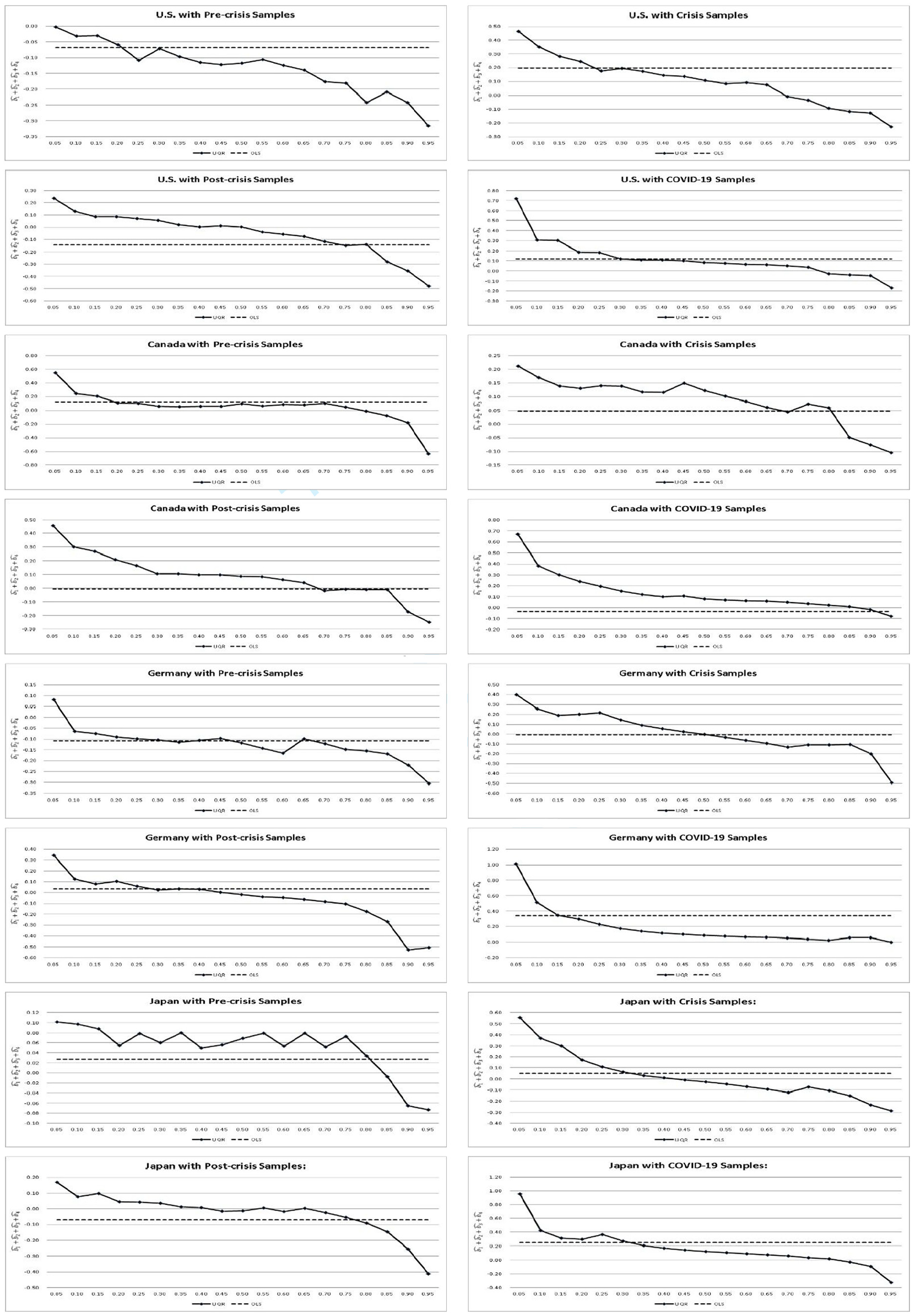
Safe-haven effect of gold of UQR estimates (solid lines) versus OLS estimates (dotted lines) across quantiles. Over all subperiods, the estimates of b1 + b2 + b3 + b4 generally decrease with the quantiles of return distribution of gold, implying that the safe-haven effect is asymmetric and is maximized at around the uppermost quantiles (0.9–0.95).

Safe-haven effect of USD of UQR estimates (solid lines) versus OLS estimates (dotted lines) across quantiles. Over all subperiods, the estimates of b1 + b2 + b3 + b4 generally decrease with the quantiles of return distribution of USD, implying that the safe-haven effect is asymmetric and is maximized at around the uppermost quantiles (0.9–0.95).

Safe-haven effect of bonds of UQR estimates (solid lines) versus OLS estimates (dotted lines) across quantiles. Over all subperiods, the estimates of b1 + b2 + b3 + b4 generally decrease with the quantiles of return distribution of bonds, implying that the safe-haven effect is asymmetric and is maximized at around the uppermost quantiles (0.9–0.95).

Safe-haven effect of crude oil of UQR estimates (solid lines) versus OLS estimates (dotted lines) across quantiles. Over all subperiods, the estimates of b1 + b2 + b3 + b4 generally decrease with the quantiles of return distribution of crude oil, implying that the safe-haven effect is asymmetric and is maximized at around the uppermost quantiles (0.9–0.95).

Safe-haven effect of Bitcoin of UQR estimates (solid lines) versus OLS estimates (dotted lines) across quantiles. Over all subperiods, the estimates of b1 + b2 + b3 + b4 generally decrease with the quantiles of return distribution of Bitcoin, implying that the safe-haven effect is asymmetric and is maximized at around the uppermost quantiles (0.9–0.95).
From the UQR estimation results, we observe that gold, the USD, and bonds serve as weak safe havens against stocks for all countries over all periods when they exceed specific thresholds, supporting Hypothesis 3A, 3B, 3C, and 4. For example, prior to the GFC, gold was a weak safe haven for the U.S., Canada, Germany, and Japan when its returns were larger than 5%, 80%, 10%, and 80% quantiles, respectively. In addition, we find that the safe-haven ability of gold and bonds weakened during the GFC, perhaps due to their bidirectional interdependence with stocks (Choudhry et al., 2015). The increased safe-haven ability of the USD during the GFC may be the result of the USD appreciation in the second half of 2008 (Fratzscher, 2009; McCauley & McGuire, 2009).
The weak safe-haven effect of crude oil against stocks is confirmed for all countries at the upper quantiles of oil returns before the GFC, but is greatly diminished over the crisis and post-crisis periods. This finding, which partially supports Hypothesis 3D and 4, may suggest that the stock-oil linkage increased because of the global financial turmoil (Creti et al., 2013; Filis et al., 2011; Kolodziej et al., 2014).
Bitcoin serves as a weak safe-haven for stocks investors in the U.S., Canada, and Germany when its returns are in the upper quantile, supporting Hypothesis 3E and 4. For example, Bitcoin is a safe haven for the U.S., Canada, and Germany post-GFC when its returns are higher than 90%, 85%, and 85% quantile levels, respectively, which is consistent with findings in Baur et al. (2018).
Results of Flight/Contagion Analysis
This study investigates contagion/flight using the definition provided by Baur and Lucey (2009). Table 7 provides the estimation results of contagion/flight for gold, the USD, bonds and crude oil. In the OLS estimation, a flight to the USD is found in Germany. In contrast, we observe stock-gold contagion in Japan and stock-oil contagion in Germany and Japan.
Summary results of contagion/flight.

Note. This table summarizes contagion/flights for three countries. Contagion/flight status is evaluated by justifying the signs of
Using the UQR estimation, the results can be categorized into two situations. First, stock-gold, stock-bonds, and stock-oil contagion is found at lower quantiles of returns of gold, bonds and crude oil, respectively. However, a decoupling can be observed in stock-gold and stock-oil pairs at upper quantiles. Second, a flight from stocks to the USD is supported at upper quantiles for all countries.
The stock-gold, stock-bonds, and stock-oil contagion observed at lower quantiles of returns for gold, bonds, and crude oil may be explained by a change in investors’ appetite for risk (Kumar & Persaud, 2002). When the returns of these assets hit bottom in a crisis period, investors’ risk appetite for those assets likely declines, so investors may, on average, reduce their exposure to these assets, leading to contagion. In contrast, a flight from stocks to the USD seen identified for all countries with different country-specific thresholds of the USD returns. Flight-to-safety (Baele et al., 2020) may provide insights of this finding because the USD was considered a high quality, liquid asset during and after the GFC. Hence, flight from stocks to the USD is consistent with a flight to safety.
Asymmetric Hedging, Safe-Haven, Contagion, and Flight-to-Quality Effect
Asymmetric hedging and safe-haven properties are observed from Figures 1 to 10. Figures 1 to 5 clearly show that over all subperiods, the estimates of
Figures 6 to 10 clearly show the asymmetry in the safe-haven effects of the considered assets. The estimates of
The findings of asymmetry in hedges and safe havens reveal that OLS (or conditional mean estimator) is unable to include heterogeneity in the return distribution of considered assets (Badshah, 2013). For example, OLS underestimate the hedging effect of each asset for the U.S., Canada, and Germany at the low quantiles; however, it overestimates the hedging effect for all countries at high quantiles. Conversely, OLS overestimates the safe-haven effect at lower quantiles and underestimates this effect at the upper quantiles. Consequently, our findings reject the use of OLS for short-term safe-haven analysis, despite the fact that it is widely used in the literature, because it may have mis-estimated hedging and safe-haven relationships at the upper/lower quantiles of a return distribution.
Finally, we observe the existence of asymmetric contagion/flight based on the findings in Table 7. For example, we see stock-gold, stock-bond and stock-oil contagion at low quantile that diminishes at high quantile. This finding implies that conventional “safe” assets such as gold and bonds act as safe havens only when their returns are sufficiently high, and may experience contagion with stocks if these asset markets are also in the turmoil. By contrast, a flight from stocks to the USD is identified for all countries when the USD returns are sufficiently high.
Summary
The results of the OLS and UQR estimations jointly indicate that gold could serve at least as a weak hedging asset against stocks for all considered countries over all subperiods, consistent with results in Baur and Lucey (2010) and others. Nevertheless, conflicting results of the hedging analysis between OLS and UQR are found for pre-crisis Canada; the results of the OLS estimation show that gold could not act as a hedge against stocks during this period, although the UQR estimation shows that gold acted as a strong hedge at the lower quantiles of the gold-return distribution. A possible explanation for this finding is that the OLS determines relationships at the mean, whereas the UQR estimates the quantile function, accounting for heterogeneity in the gold-return distribution.
Another interesting finding is gold’s hedging ability for the U.S. after the GFC. Although gold’s strong hedging ability is confirmed by the UQR estimation, adding gold to a portfolio would not improve the diversification because gold only hedges stocks in a bearish gold market. Therefore, gold’s hedging ability is not valid for the U.S. after the GFC.
Moreover, after the GFC gold could not offer a hedging ability for stocks in the U.S., Canada and Germany at the upper quantile of the gold-return distribution. That is, gold co-moves with stocks in the U.S., Canada, and Germany on average at the upper quantile of the gold-return distribution. This finding indicates that, for the U.S., Canada, and Germany, gold and stocks tend to exhibit positive interdependence on average in a bullish gold market, in accordance with Hussain Shahzad et al. (2017)
The UQR estimation reveals weak safe-haven properties of gold, the USD, bonds, and Bitcoin for all considered countries post-GFC, particularly at the high quantiles of the return distribution. It is well documented that an increasing price may be interpreted as a signal of safe-haven purchases (Baur, 2012a), implying that high asset returns may be an indicator of high demand of safe-haven purchases. Hence, the significance of the safe-haven abilities seen in the upper quantile of return distribution for the assets considered demonstrates the importance of the UQR estimation approach for a safe-haven analysis.
The UQR estimations show that the USD was the most efficient safe haven during the crisis period. For U.S. equity market, the UQR characterizes the safe-haven role of the USD when USD returns are above the 30% quantile; while the UQR characterizes the USD’s safe-haven role for equity markets in Canada, Germany and Japan over all quantile of the USD return distribution. A possible explanation is that capital tends to move into large-developed countries such as the U.S. when global markets are down, leading to appreciation of the USD. This generates a negative correlation between the USD and equity markets (Cho et al., 2016).
The USD is a safe-haven asset against stocks in both pre- and post-crisis periods. The fundamental factors driving the USD’s safe-haven role before the GFC differ from those after the GFC. Before the GFC, despite the emergence of the euro, the USD continued to be the world’s most dominant currency, playing a central role in international trade as a store of value, medium of exchange, and shelter for investors when other markets decline. However, the uncertainty in equity and bond markets, stemming from the financial crisis, highlights the importance of holding cash, and therefore enhances flight to the USD.
The asymmetric contagion/flight pattern is connected to the asymmetric safe-haven property discussed above. Specifically, if an asset’s safe-haven ability during the GFC was weaker than the aggregate safe-haven ability during the pre- and post-crisis periods, an asymmetric contagion between this asset and stocks exists. Whereas, if the safe-haven ability of an asset is stronger during the GFC than in non-crisis periods, an asymmetric flight from stocks to this asset occurs.
Finally, the quantile estimates’ changing properties present an interesting picture of how the asset-return distribution depend on changing conditions in the various stock markets. The impact of stock returns during normal verse extremely adverse market conditions on each asset’s returns varies and is highly asymmetric over all subperiods. This finding may be better explained by investor behavior.
Interpretation for Asymmetric Hedging and Safe-Haven Relations
The aforementioned results show that gold, the USD, bonds, and Bitcoin typically serve as hedges against stocks at the lower quantile of their respective return distributions. In other words, since the financial crisis the return series for each of these assets versus the stock markets for the countries included in this analysis have exhibited a negative relationship, on average, when performance for the asset is poor. Traditionally, a safe asset with an inverse asymmetric volatility-return relationship is viewed as a good hedging instrument if its volatility is low. Investors often use such assets tactically with the goal of preserving wealth during market corrections, and times of geopolitical stress or persistent dollar weakness. Investors who suffered substantial losses in the equity market during the GFC are eager to find safe alternatives to hedge their equity exposures. Hence, investors tend to put more capital in safe assets when those asset markets appear to have hit the bottom. Our empirical findings may be explained by the representativeness heuristics, which involves an overreliance on stereotypes or “rules of thumb” to make quick, often irrational judgments (Shefrin, 2008; Tversky & Kahneman, 1974).
Investor behaviors could be a possible reason to explain the asymmetric hedging property. As returns for hedging assets increase, investors may become more focused on pursuing those returns and thus overlook the original purpose (i.e., the hedging function) of holding these assets. This change in investor behavior may affect the price and volatilities of hedging assets, further reducing their hedging ability.
We also find that stock-gold, and stock-Bitcoin pairs co-move at the high quantiles of the gold and Bitcoin return distributions, especially during the post-crisis period, indicating the possible inflation-hedging ability of these assets, (Hoang et al., 2016; Ji & Chun, 2016). After the GFC, quantitative easing (QE) was widely adopted by many central banks, producing various financial and monetary effects through QE’s impact on financial market prices. For example, QE is credited with boosting stock market returns as well as inflation. Therefore, when a central bank embarks on QE, stock prices as well as gold (and Bitcoin) prices may rise simultaneously because of increasing incentives for investors to buy gold (Bitcoin).
Apart from the asymmetric hedging relationship, investors’ loss aversion may be a reasonable explanation for the asymmetric safe-haven property (Kahneman & Tversky, 1979; Tversky & Kahneman, 1991). When the returns of safe-haven assets increase, they may attract more investors. The increased demand could strengthen the asset’s role as a safe haven because more investors seek to hold the asset to help minimize losses in times of market stress.
Robustness Check
To test the robustness of the UQR estimations, we further analyze the hedging/safe-haven effects by adding lagged stock returns as explanatory variables in the UQR model. This allows us to see whether the interactivity of contemporaneous and lagged stock returns impact the UQR estimation. For example, the augmented UQR model for gold is given by

Figures 11 to 15 report the estimation results of contemporaneous hedging/safe-haven effects in this augmented version of the UQR model. The contemporaneous hedging/safe-haven effects are systematically consistent with those in the UQR, as reported in Figures 1 to 10. These results indicate that the UQR model generally holds when lagged stock returns are included as explanatory variables.
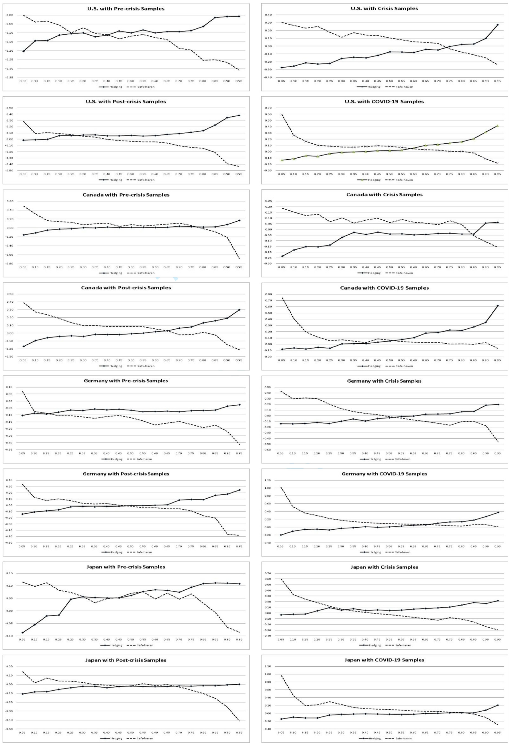
Robust check of hedging and safe-haven effects of gold across quantiles. The solid lines stand for the hedging effect, and the dotted lines stand for the safe-haven effect.

Robust check of hedging and safe-haven effects of USD across quantiles. The solid lines stand for the hedging effect, and the dotted lines stand for the safe-haven effect.

Robust check of hedging and safe-haven effects of bonds across quantiles. The solid lines stand for the hedging effect, and the dotted lines stand for the safe-haven effect.
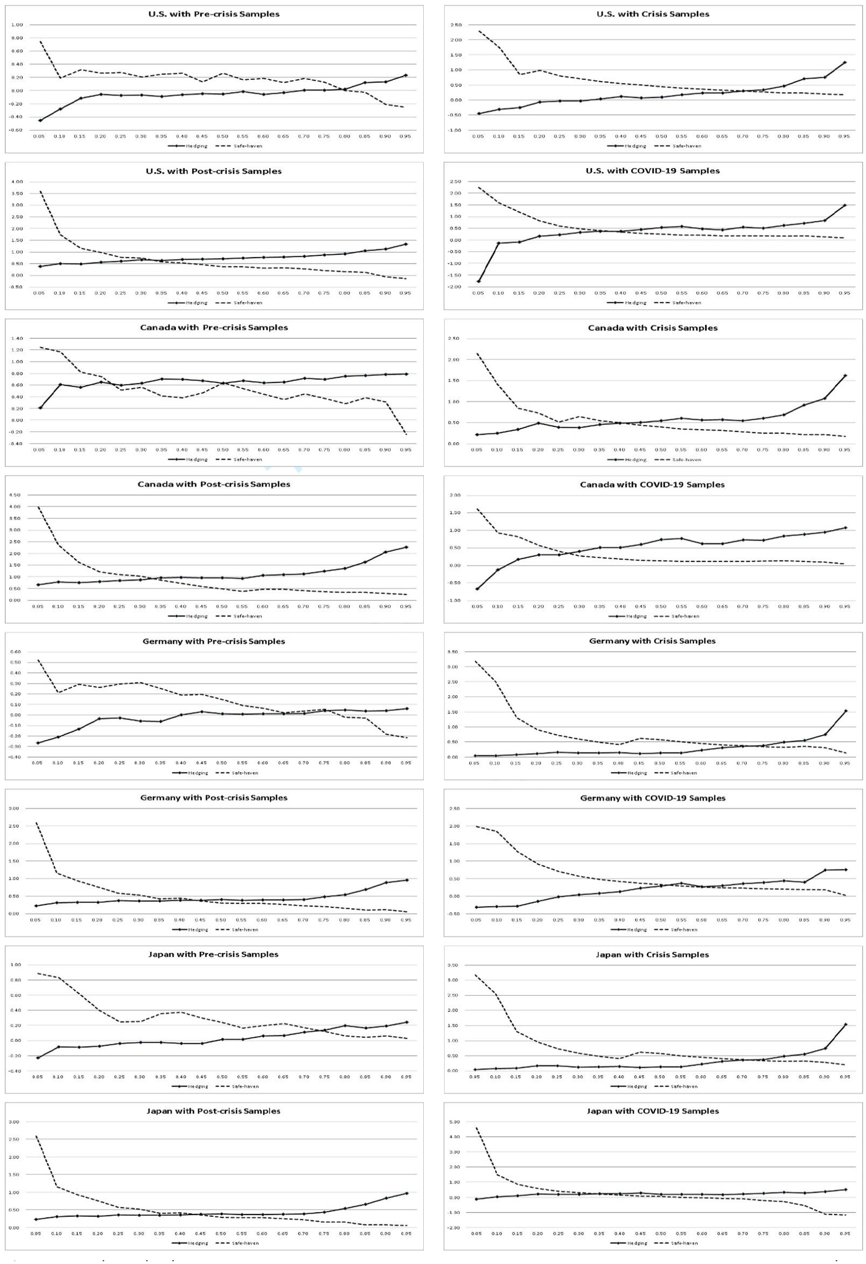
Robust check of hedging and safe-haven effects of crude oil across quantiles. The solid lines stand for the hedging effect, and the dotted lines stand for the safe-haven effect.
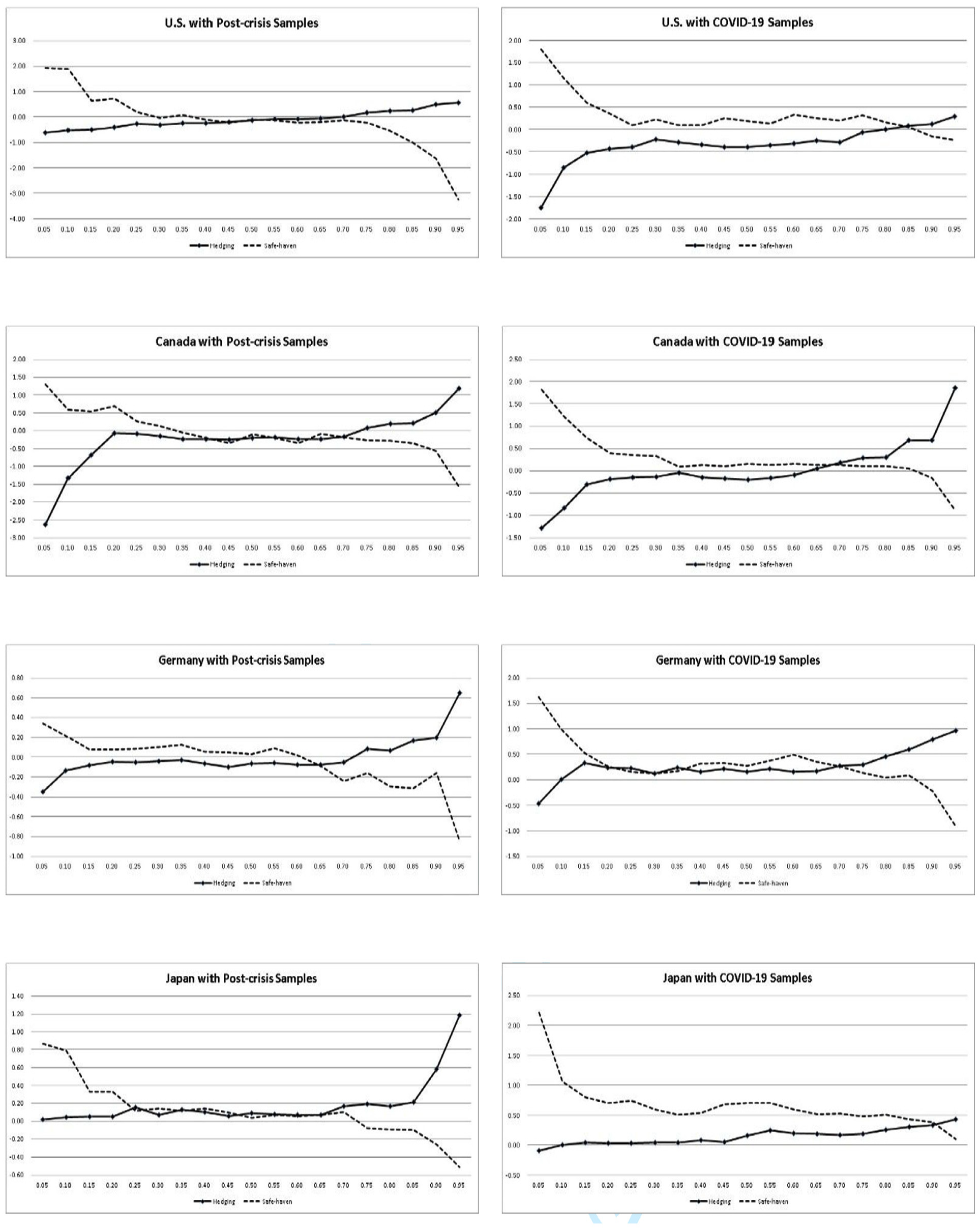
Robust check of hedging and safe-haven effects of Bitcoin across quantiles. The solid lines stand for the hedging effect, and the dotted lines stand for the safe-haven effect.
Conclusion
This study contributes to the literature on risk management in financial markets by examining the asymmetric relationships between gold, the USD, bonds, and Bitcoin returns versus stock market returns in four developed countries, and their asymmetric flight-to-quality and contagion effects. Our findings show that, compared with the standard approach of modeling hedging/safe-haven relationships using OLS, UQR provides additional insights regarding the potential heterogeneous correlations between stock returns and the return distribution of tested assets. Our results reveal asymmetric hedging/safe-haven effects of these assets against stocks, implying that OLS regression may over- or under-estimate an asset’s hedging/safe-haven ability at the extremes of the return distribution. In addition, cross-asset flight-to-quality and contagion is not symmetric across all quantiles of these asset returns. In other words, using a conditional mean estimator to analyze flights or contagion may miss important information at the extreme quantiles of asset returns.
Our findings offer important guidelines and implications for investing using safe-haven assets. Safe havens and hedges are two common strategies used to limit losses. Although it is widely accepted that the conventional safe-haven assets, such as gold, the USD, the government bonds, etc., retain or increase their value in times of market turbulence, the assets that are actually considered safe havens can vary depending on their specific nature. In other words, whether investors can successfully protect their returns and minimize the impact of adverse market conditions relies not only on the types of hedges and safe-havens assets used, but also the market conditions (bear, normal, or bull) for those assets. Based on our findings, investors would be wise to regularly monitor changes in the returns of hedges or safe havens, and could use such observations to ensure better, more profitable speculation strategies.
Although our study revisits the hedging/safe-haven properties of wildly recognized safe-haven assets using a more robust approach, some limitations imposed by the models are unavoidable. For example, the linear parametric functional form is proposed for a RIF regression. A nonparametric RIF regression could be a solution to release this limitation. This can be an interesting topic for future theoretical research.
Footnotes
Appendix
Estimation results of UQR model (full samples)

| OLS | Quantile | |||||||||||
|---|---|---|---|---|---|---|---|---|---|---|---|---|
| 5th | 10th | 20th | 30th | 40th | 50th | 60th | 70th | 80th | 90th | 95th | ||
| Panel A: gold | ||||||||||||
| Panel A.1: U.S. | ||||||||||||
| b 1 | 0.0560*** (0.0131) | −0.1623*** (0.0212) | −0.1007*** (0.0133) | −0.0726*** (0.0065) | −0.0422*** (0.0034) | 0.0018 (0.0019) | 0.0182*** (0.0017) | 0.0275*** (0.0026) | 0.0519*** (0.0027) | 0.0952*** (0.0042) | 0.2422*** (0.0081) | 0.3298*** (0.0174) |
| b 2 | −0.1452** (0.0681) | 0.3825*** (0.0625) | 0.1025*** (0.0292) | 0.1243*** (0.0164) | −0.0217*** (0.0060) | −0.0221*** (0.0055) | −0.0663*** (0.0068) | −0.1086*** (0.0133) | −0.1615*** (0.0104) | −0.3798*** (0.0239) | −0.5147*** (0.0275) | −0.5419*** (0.0514) |
| b 3 | 0.1292** ( 0.0614) | 0.0522 (0.0441) | 0.3221*** (0.0155) | 0.1217*** (0.0138) | 0.2106*** (0.0075) | 0.0842*** (0.0079) | 0.0792*** (0.0074) | 0.0762*** (0.0152) | 0.0443*** (0.0135) | 0.1861*** (0.0156) | 0.1109*** (0.0232) | −0.0092 (0.0290) |
| b 4 | 0.0036 (0.0443) | 0.4216*** (0.0339) | 0.0841 (0.0662) | −0.0521*** (0.0074) | −0.0961*** (0.0050) | −0.0170 (0.0154) | 0.0014*** (0.0033) | 0.0120 (0.0079) | 0.0198*** (0.0030) | −0.0015 (0.0049) | −0.0100 (0.0113) | −0.0701** (0.0312) |
| Panel A.2: Canada | ||||||||||||
| b 1 | −0.0097 (0.199) | −0.3020*** (0.0369) | −0.1690*** (0.0146) | −0.0614*** (0.0050) | −0.0337*** (0.0049) | −0.0117*** (0.0027) | −0.0084*** (0.0022) | 0.0225*** (0.0017) | 0.0556*** (0.0039) | 0.0992*** (0.0029) | 0.1760*** (0.0092) | 0.2448*** (0.0098) |
| b 2 | 0.0091 (0.0387) | 0.3273*** (0.0414) | 0.2948*** (0.0292) | 0.1415*** (0.0085) | 0.0675*** (0.0139) | 0.0701*** (0.0077) | 0.0758*** (0.0088) | 0.0130*** (0.0061) | −0.1024*** (0.0193) | −0.2868*** (0.0195) | −0.2367*** (0.0246) | −0.1800 (0.3048) |
| b 3 | −0.0040 (0.0104) | 0.2855*** (0.0460) | 0.1004** (0.0438) | 0.1308*** (0.0130) | 0.0658*** (0.0077) | 0.0173*** (0.0032) | −0.0305 (0.0131) | −0.0403*** (0.0093) | −0.0012 (0.0073) | 0.0775*** (0.0201) | −0.1676*** (0.0316) | −0.3072*** (0.0577) |
| b 4 | 0.0970*** (0.0322) | 0.6087*** (0.0675) | 0.1405*** (0.0571) | −0.0728 (0.0623) | −0.0185*** (0.0031) | −0.0388*** (0.0063) | 0.0045 (0.0055) | 0.0213*** (0.0035) | 0.0357*** (0.0079) | 0.0480*** (0.0056) | 0.0220 (0.0231) | −0.0354 (0.0248) |
| Panel A.3: Germany | ||||||||||||
| b 1 | −0.0235 (0.0187) | −0.1842*** (0.0123) | −0.1333*** (0.0113) | −0.0704*** (0.0039) | −0.0133*** (0.0028) | −0.0130*** (0.0022) | −0.0033*** (0.0010) | 0.0132*** (0.0027) | 0.0551*** (0.0023) | 0.0772*** (0.0037) | 0.1657*** (0.0053) | 0.1918*** (0.0086) |
| b 2 | 0.1112*** (0.0219) | 0.8731*** (0.0899) | 0.6943*** (0.0383) | 0.4114*** (0.0198) | 0.1886*** (0.0093) | 0.0954*** (0.0084) | 0.0610*** (0.0045) | 0.0059 (0.0089) | −0.0936*** (0.0060) | −0.1359*** (0.0118) | −0.2111*** (0.0103) | −0.2895*** (0.0185) |
| b 3 | −0.1822*** (0.0331) | −0.1857** (0.0827) | −0.2568*** (0.0220) | −0.2276*** (0.0121) | −0.1332*** (0.0067) | −0.0704*** (0.0077) | −0.0658*** (0.0050) | −0.0609*** (0.0046) | −0.0241*** (0.0035) | −0.0782*** (0.0100) | −0.2701*** (0.0141) | −0.2863*** (0.0271) |
| b 4 | 0.0614 (0.0053) | 0.1769*** (0.0243) | 0.0512 (0.0429) | 0.0324*** (0.0033) | 0.0304*** (0.0041) | 0.0327*** (0.0034) | 0.0256*** (0.0015) | 0.0294*** (0.0037) | 0.0163*** (0.0037) | 0.0173*** (0.0054) | 0.0568*** (0.0104) | 0.0002 (0.0171) |
| Panel A.4: Japan | ||||||||||||
| b 1 | 0.0264 (0.0170) | −0.1166*** (0.0169) | −0.0705*** (0.0107) | −0.0487*** (0.0029) | −0.0094*** (0.0026) | −0.0111*** (0.0019) | −0.0017 (0.0015) | −0.0002 (0.0022) | 0.0140*** (0.0023) | 0.0549*** (0.0038) | 0.0833*** (0.0079) | 0.1876*** (0.0129) |
| b 2 | −0.1082** (0.0467) | 0.2856*** (0.0491) | 0.0289*** (0.0104) | 0.0206*** (0.0065) | −0.0313*** (0.0075) | −0.0513*** (0.0065) | −0.0704*** (0.0038) | −0.1299*** (0.0038) | −0.1705*** (0.0045) | −0.3390*** (0.0115) | −0.3972*** (0.0179) | −0.5509*** (0.0490) |
| b 3 | 0.0750 (0.0514) | 0.2047** (0.0444) | 0.2956*** (0.0120) | 0.1466*** (0.0041) | 0.0847*** (0.0027) | 0.0692*** (0.0048) | 0.0488*** (0.0033) | 0.0765*** (0.0032) | 0.0515*** (0.0044) | 0.1095*** (0.0085) | 0.0789*** (0.0178) | 0.1622*** (0.0216) |
| b 4 | 0.0413 (0.0418) | 0.1340*** (0.0471) | 0.0012 (0.0113) | −0.0035 (0.0033) | 0.0204*** (0.0022) | 0.0198*** (0.0026) | 0.0250*** (0.0037) | 0.0371*** (0.0027) | 0.0432*** (0.0070) | 0.0210*** (0.0051) | −0.0011 (0.0222) | −0.0741*** (0.0226) |
| Panel B: USD | ||||||||||||
| Panel B.1: U.S. | ||||||||||||
| b 1 | −0.0761*** (0.0052) | −0.1683*** (0.0071) | −0.1468*** (0.0039) | −0.0944*** (0.0023) | −0.0721*** (0.0014) | −0.0606*** (0.0014) | −0.0517*** (0.0011) | −0.0497*** (0.0011) | −0.0519*** (0.0012) | −0.0475*** (0.0016) | −0.0320*** (0.0025) | −0.0329*** (0.0038) |
| b 2 | 0.0050 (0.0119) | 0.1326*** (0.0098) | 0.0887*** (0.0046) | 0.0761*** (0.0045) | 0.0488*** (0.0021) | 0.0208*** (0.0016) | −0.0027*** (0.0009) | −0.0219 (0.0010) | −0.0444*** (0.0025) | −0.0950*** (0.0040) | −0.1200*** (0.0055) | −0.1996*** (0.0178) |
| b 3 | −0.0238** (0.0117) | 0.0068 (0.0064) | 0.0337*** (0.0038) | −0.0080*** (0.0014) | −0.0085*** (0.0021) | −0.0016 (0.0019) | −0.0001 (0.0016) | 0.0175*** (0.0013) | 0.0090 (0.0024) | 0.0050*** (0.0010) | −0.0633*** (0.0027) | −0.1902*** (0.0093) |
| b 4 | −0.0347*** (0.0089) | 0.0245*** (0.0035) | 0.0172*** (0.0025) | 0.0070*** (0.0021) | 0.0070*** (0.0022) | 0.0104*** (0.0008) | 0.0165*** (0.0014) | 0.0062*** (0.0013) | 0.0233*** (0.0020) | 0.0293*** (0.0014) | 0.0278*** (0.0045) | 0.0634*** (0.0106) |
| Panel B.2: Canada | ||||||||||||
| b 1 | −0.2190*** (0.0166) | −0.5429*** (0.0408) | −0.3474*** (0.0195) | −0.2816*** (0.0097) | −0.2284*** (0.0061) | −0.1802*** (0.0067) | −0.1672*** (0.0040) | −0.1589*** (0.0042) | −0.1427*** (0.0048) | −0.1246*** (0.0055) | −0.0893*** (0.0056) | −0.0669*** (0.0058) |
| b 2 | −0.0796*** (0.0238) | 0.3930*** (0.0286) | 0.2184*** (0.0198) | 0.1218*** (0.0056) | 0.0381*** (0.0036) | −0.0116*** (0.0041) | −0.0603*** (0.0012) | −0.1073*** (0.0039) | −0.1957*** (0.0068) | −0.3366*** (0.0113) | −0.4153*** (0.0197) | −0.6312*** (0.0464) |
| b 3 | 0.0491*** (0.0102) | 0.1594*** (0.0141) | 0.0973*** (0.0073) | 0.0901*** (0.0058) | 0.1022*** (0.0042) | 0.0826*** (0.0094) | 0.1025*** (0.0018) | 0.0898*** (0.0072) | 0.0904*** (0.0036) | 0.0905*** (0.0122) | −0.1079*** (0.0227) | −0.1754*** (0.0332) |
| b 4 | 0.0179 (0.0454) | −0.0473*** (0.0093) | −0.0080*** (0.0023) | 0.0158*** (0.0018) | 0.0329*** (0.0024) | 0.0448*** (0.0021) | 0.0514*** (0.0007) | 0.0834*** (0.0024) | 0.1128*** (0.0031) | 0.1774*** (0.0046) | 0.2128*** (0.0118) | 0.0503*** (0.0190) |
| Panel B.3: Germany | ||||||||||||
| b 1 | −0.0558 (0.0377) | −0.2046*** (0.0060) | −0.1452*** (0.0073) | −0.0851*** (0.0018) | −0.0593*** (0.0015) | −0.0358*** (0.0012) | −0.0280*** (0.0016) | −0.0169*** (0.0012) | −0.0134*** (0.0023) | −0.0002 (0.0025) | 0.0142*** (0.0045) | 0.0196*** (0.0028) |
| b 2 | −0.0165 (0.0289) | 0.1964*** (0.0135) | 0.1341*** (0.0131) | 0.1185*** (0.0066) | 0.0759*** (0.0033) | 0.0172*** (0.0037) | −0.0165*** (0.0031) | −0.0455*** (0.0036) | −0.1032*** (0.0068) | −0.1399*** (0.0080) | −0.2253*** (0.0179) | −0.3944*** (0.0421) |
| b 3 | 0.0223 (0.0301) | 0.2144*** (0.0147) | 0.1193*** (0.0071) | 0.0190 (0.0256) | −0.0056*** (0.0016) | 0.0104*** (0.0022) | 0.0167*** (0.0012) | 0.0076** (0.0019) | 0.0271*** (0.0040) | 0.0010 (0.0018) | 0.0039 (0.0185) | 0.0163 (0.0289) |
| b 4 | −0.0691*** (0.0093) | −0.1625*** (0.0093) | −0.1010*** (0.0072) | −0.0787*** (0.0033) | −0.0466*** (0.0023) | −0.0415*** (0.0019) | −0.0218*** (0.0018) | −0.0165*** (0.0014) | −0.0292*** (0.0050) | −0.0323*** (0.0028) | −0.0805*** (0.0113) | −0.1558*** (0.0260) |
| Panel B.4: Japan | ||||||||||||
| b 1 | 0.1020*** (0.0094) | 0.0541*** (0.0073) | 0.0667*** (0.0038) | 0.0700*** (0.0029) | 0.0695*** (0.0021) | 0.0706*** (0.0022) | 0.0710*** (0.0018) | 0.0768*** (0.0021) | 0.0911*** (0.0026) | 0.1052*** (0.0037) | 0.1694*** (0.0070) | 0.2355*** (0.0169) |
| b 2 | −0.0220 (0.0259) | 0.0899*** (0.0196) | 0.1860*** (0.0106) | 0.0827*** (0.0064) | 0.0271*** (0.0045) | 0.0069*** (0.0012) | −0.0026 (0.0035) | −0.0456*** (0.0032) | −0.0672*** (0.0031) | −0.0800*** (0.0059) | −0.1282*** (0.0093) | −0.1922*** (0.0233) |
| b 3 | 0.0481 (0.0385) | 0.3724*** (0.0295) | 0.0780*** (0.0104) | 0.0100 (0.0253) | 0.0083*** (0.0021) | −0.0034*** (0.0011) | −0.0224*** (0.0027) | 0.0020 (0.0040) | 0.0085*** (0.0024) | 0.0133 (0.0167) | −0.0224*** (0.0039) | −0.0506** (0.0248) |
| b 4 | −0.0429 (0.0432) | −0.0956 (0.0920) | −0.0989*** (0.0057) | −0.0492*** (0.0028) | −0.0361*** (0.0025) | −0.0343*** (0.0016) | −0.0173*** (0.0008) | −0.0136*** (0.0027) | −0.0304*** (0.0019) | −0.0483*** (0.0019) | −0.0738*** (0.0031) | −0.1133*** (0.0227) |
| Panel C: bonds | ||||||||||||
| Panel C.1: U.S. | ||||||||||||
| b 1 | −0.1047*** (0.0081) | −0.2604*** (0.0218) | −0.1774*** (0.0121) | −0.1263*** (0.0057) | −0.1162*** (0.0043) | −0.1073*** (0.0036) | −0.0992*** (0.0033) | −0.0920*** (0.0027) | −0.0813*** (0.0034) | −0.0722*** (0.0038) | −0.0458*** (0.0035) | −0.0129*** (0.0039) |
| b 2 | −0.0578 (0.0432) | 0.4197*** (0.0367) | 0.2116*** (0.0147) | 0.0864*** (0.0064) | 0.0397*** (0.0052) | −0.0112*** (0.0022) | −0.0361*** (0.0042) | −0.0983*** (0.0032) | −0.1406*** (0.0041) | −0.2083*** (0.0066) | −0.3673*** (0.0119) | −0.5339*** (0.0261) |
| b 3 | 0.0110 (0.0149) | −0.1381*** (0.0157) | −0.0540*** (0.0057) | −0.0013*** (0.0025) | 0.0080*** (0.0015) | 0.0309*** (0.0031) | 0.0367*** (0.0028) | 0.0544*** (0.0030) | 0.0454 (0.0052) | 0.0389*** (0.0064) | 0.0815*** (0.0061) | −0.0565*** (0.0118) |
| b 4 | 0.0326 (0.291) | 0.0438*** (0.0075) | 0.0486*** (0.0045) | 0.0401*** (0.0028) | 0.0476*** (0.0027) | 0.0508*** (0.0032) | 0.0581*** (0.0030) | 0.0810*** (0.0036) | 0.0950*** (0.0038) | 0.1088*** (0.0067) | 0.0838*** (0.0089) | 0.1550 (0.0979) |
| Panel C.2: Canada | ||||||||||||
| b 1 | −0.0713*** (0.0076) | −0.1209*** (0.0106) | −0.1097*** (0.0077) | −0.1060*** (0.0058) | −0.0796*** (0.0053) | −0.0749*** (0.0056) | −0.0636*** (0.0053) | −0.0860*** (0.0039) | −0.0628*** (0.0026) | −0.0520*** (0.0032) | −0.0394*** (0.0024) | −0.0183*** (0.0031) |
| b 2 | −0.0305 (0.0495) | 0.1513*** (0.0142) | 0.1078*** (0.0078) | 0.0644*** (0.0050) | 0.0047*** (0.0014) | −0.0237*** (0.0028) | −0.0267*** (0.0094) | −0.0411*** (0.0057) | −0.0614*** (0.0048) | −0.1372*** (0.0048) | −0.2476*** (0.0089) | −0.2787*** (0.0150) |
| b 3 | −0.0167 (0.0198) | −0.0438*** (0.0086) | −0.0321*** (0.0033) | −0.0104*** (0.0021) | −0.0005 (0.0017) | 0.0012 (0.0020) | 0.0001 (0.0022) | −0.0023 (0.0017) | 0.0046 (0.0029) | −0.0010 (0.0037) | −0.0100 (0.0094) | 0.0091 (0.0155) |
| b 4 | 0.0499*** (0.0071) | 0.0238*** (0.0046) | 0.0370*** (0.0030) | 0.0377*** (0.0015) | 0.0516*** (0.0039) | 0.0675*** (0.0041) | 0.0604*** (0.0055) | 0.0792*** (0.0026) | 0.0711*** (0.0028) | 0.0967*** (0.0056) | 0.1396*** (0.0062) | 0.0153 (0.0265) |
| Panel C.3: Germany | ||||||||||||
| b 1 | −0.0263*** (0.0054) | −0.0568*** (0.0017) | −0.0517*** (0.0011) | −0.0440*** (0.0005) | −0.0408*** (0.0006) | −0.0363*** (0.0005) | −0.0356*** (0.0005) | −0.0353*** (0.0006) | −0.0322*** (0.0006) | −0.0235*** (0.0006) | −0.0145*** (0.0010) | −0.0093*** (0.0004) |
| b 2 | −0.0192*** (0.0013) | 0.0721*** (0.0018) | 0.0539*** (0.0018) | 0.0329*** (0.0005) | 0.0151*** (0.0012) | 0.0038*** (0.0011) | −0.0077*** (0.0012) | −0.0209*** (0.0022) | −0.0377*** (0.0015) | −0.0464*** (0.0013) | −0.0509*** (0.0020) | −0.0758*** (0.0049) |
| b 3 | 0.0124 (0.0231) | −0.0020 (0.0026) | 0.0016 (0.0019) | 0.0032*** (0.0007) | 0.0064*** (0.0006) | 0.0056*** (0.0006) | 0.0068*** (0.0009) | 0.0077*** (0.0009) | 0.0091*** (0.0007) | −0.0044*** (0.0013) | −0.0339*** (0.0031) | −0.0414*** (0.0030) |
| b 4 | 0.0239 (0.0383) | −0.0022*** (0.0008) | −0.0047*** (0.0004) | 0.0011*** (0.0003) | 0.0083*** (0.0003) | 0.0141*** (0.0006) | 0.0179*** (0.0004) | 0.0246*** (0.0003) | 0.0277*** (0.0004) | 0.0275*** (0.0004) | 0.0268*** (0.0015) | 0.0223*** (0.0026) |
| Panel C.4: Japan | ||||||||||||
| b 1 | −0.0151*** (0.0032) | −0.0432*** (0.0055) | −0.0292*** (0.0026) | −0.0243*** (0.0014) | −0.0199*** (0.0008) | −0.0144*** (0.0006) | −0.0127*** (0.0004) | −0.0123*** (0.0003) | −0.0109*** (0.0006) | −0.0094*** (0.0011) | −0.0038*** (0.0012) | 0.0048*** (0.0013) |
| b 2 | −0.0131 (0.0289) | 0.0401*** (0.0044) | 0.0182*** (0.0033) | 0.0147*** (0.0019) | 0.0075*** (0.0012) | −0.0021** (0.0010) | −0.0057*** (0.0016) | −0.0191*** (0.0008) | −0.0235*** (0.0016) | −0.0465*** (0.0030) | −0.0637*** (0.0025) | −0.0805** (0.0036) |
| b 3 | 0.0204 (0.0338) | 0.0085*** (0.0013) | 0.0180*** (0.0023) | 0.0202*** (0.0024) | 0.0116*** (0.0007) | 0.0097*** (0.0003) | 0.0076*** (0.0009) | 0.0137*** (0.0009) | 0.0115*** (0.0016) | 0.0268*** (0.0036) | 0.0409*** (0.0035) | 0.0276*** (0.0047) |
| b 4 | 0.0031 (0.0079) | 0.0108*** (0.0024) | −0.0002 (0.0014) | −0.0041*** (0.0011) | 0.0038*** (0.0009) | 0.0049*** (0.0004) | 0.0072*** (0.0005) | 0.0094*** (0.0004) | 0.0127*** (0.0011) | 0.0102*** (0.0015) | −0.0157*** (0.0033) | −0.0251*** (0.0049) |
| Panel D: crude oil | ||||||||||||
| Panel D.1: U.S. | ||||||||||||
| b 1 | 0.4999*** (0.0415) | −0.0175 (0.0280) | 0.1925*** (0.0131) | 0.2872*** (0.0138) | 0.3590*** (0.0094) | 0.4061*** (0.0094) | 0.4587*** (0.0089) | 0.4921*** (0.0110) | 0.5271*** (0.0150) | 0.6730*** (0.0171) | 1.0126*** (0.0341) | 1.3586*** (0.0758) |
| b 2 | 0.0561 (0.1088) | 1.6392*** (0.0648) | 0.9865*** (0.0474) | 0.6797*** (0.0143) | 0.3330*** (0.0275) | 0.1294*** (0.0230) | −0.1022*** (0.0126) | −0.2692*** (0.0099) | −0.4320*** (0.0332) | −0.6065*** (0.0314) | −1.2253*** (0.0629) | −1.8501*** (0.0954) |
| b 3 | 0.1190 (0.0938) | −0.1746 (0.1704) | 0.2050*** (0.0381) | 0.0005 (0.0354) | 0.1320*** (0.0212) | 0.0974*** (0.0156) | 0.1504*** (0.0111) | 0.2115*** (0.0167) | 0.2820*** (0.0200) | 0.2273*** (0.0131) | 0.3400*** (0.0559) | 0.4741*** (0.0874) |
| b 4 | 0.1682** (0.0863) | 1.9302*** (0.2591) | 0.3059*** (0.0578) | −0.1030*** (0.0092) | −0.2688*** (0.0108) | −0.2455*** (0.0093) | −0.2214*** (0.0112) | −0.2254*** (0.0081) | −0.2210*** (0.0071) | −0.1933*** (0.0099) | −0.1096*** (0.0194) | −0.1543*** (0.0365) |
| Panel D.2: Canada | ||||||||||||
| b 1 | 0.8963*** (0.0451) | 0.3405*** (0.0690) | 0.5176*** (0.0318) | 0.5804*** (0.0216) | 0.6218*** (0.0205) | 0.6872*** (0.0212) | 0.7241*** (0.0211) | 0.7538*** (0.0194) | 0.8286*** (0.0270) | 1.0608*** (0.0369) | 1.5287*** (0.0614) | 2.0214*** (0.1368) |
| b 2 | 0.1147*** (0.0186) | 1.1639*** (0.0783) | 1.4305*** (0.1008) | 1.1008*** (0.0305) | 0.7393*** (0.0426) | 0.4165*** (0.0287) | 0.2504*** (0.0177) | 0.0401*** (0.0084) | −0.2509*** (0.0197) | −0.5103*** (0.0203) | −1.0663*** (0.0440) | −1.5967*** (0.1108) |
| b 3 | 0.1073*** (0.0291) | 1.7824*** (0.1619) | 0.3426*** (0.0858) | −0.1123*** (0.0235) | −0.2340*** (0.0144) | −0.2706*** (0.0184) | −0.3524*** (0.0192) | −0.2551*** (0.0126) | −0.0844*** (0.0135) | −0.1335*** (0.0219) | −0.2163*** (0.0386) | −0.4038*** (0.0606) |
| b 4 | −0.1269*** (0.0156) | 0.0869 (0.1917) | −0.5824*** (0.0629) | −0.7833*** (0.0247) | −0.5411*** (0.0185) | −0.4337*** (0.0132) | −0.3357*** (0.0103) | −0.3273*** (0.0083) | −0.3362*** (0.0102) | −0.3139*** (0.0130) | −0.2377*** (0.0199) | −0.0979 (0.0280) |
| Panel D.3: Germany | ||||||||||||
| b 1 | 0.3435*** (0.0312) | −0.1093*** (0.0121) | 0.1184*** (0.0061) | 0.2332*** (0.0071) | 0.2354*** (0.0057) | 0.2764*** (0.0057) | 0.3094*** (0.0070) | 0.3156*** (0.0078) | 0.3608*** (0.0101) | 0.4935*** (0.0144) | 0.7091*** (0.0296) | 0.9867*** (0.0494) |
| b 2 | 0.1235*** (0.0233) | 1.3606*** (0.0981) | 0.6806*** (0.0419) | 0.5302*** (0.0286) | 0.3569*** (0.0155) | 0.2675*** (0.0121) | 0.0605*** (0.0085) | −0.0533*** (0.0107) | −0.0404*** (0.0084) | −0.2478*** (0.0357) | −0.4944*** (0.0348) | −0.9912*** (0.0480) |
| b 3 | 0.1580*** (0.0124) | 0.3163*** (0.0516) | 0.5360*** (0.0396) | 0.2706*** (0.0288) | 0.1720*** (0.0109) | 0.0096 (0.0158) | 0.0313*** (0.0060) | 0.0563*** (0.0114) | −0.0595*** (0.0068) | −0.0670*** (0.0155) | −0.1039*** (0.0194) | 0.0491 (0.0442) |
| b 4 | 0.2179*** (0.0225) | 1.6242*** (0.1496) | 0.4614*** (0.0631) | −0.2238*** (0.0165) | −0.1714*** (0.0095) | −0.1009*** (0.0050) | −0.0744*** (0.0100) | −0.0583*** (0.0120) | −0.0492*** (0.0101) | −0.0117*** (0.0049) | 0.0015 (0.0442) | −0.0423 (0.0395) |
| Panel D.4: Japan | ||||||||||||
| b 1 | 0.1504*** (0.0344) | −0.0046 (0.0182) | 0.0390*** (0.0105) | 0.1012*** (0.0067) | 0.0729*** (0.0059) | 0.0926*** (0.0037) | 0.1028*** (0.0031) | 0.1114*** (0.0055) | 0.1369*** (0.0051) | 0.2132*** (0.0085) | 0.3044*** (0.0162) | 0.4987*** (0.0269) |
| b 2 | −0.0346 (0.0947) | 0.6794*** (0.0949) | 0.3935*** (0.0387) | 0.3309*** (0.0159) | 0.2046*** (0.0169) | 0.1139*** (0.0083) | 0.0168 (0.0126) | −0.0283*** (0.0061) | −0.1685*** (0.0203) | −0.2979*** (0.0152) | −0.6125*** (0.0216) | −0.9864*** (0.0732) |
| b 3 | 0.1849 (0.2041) | 0.3379*** (0.0567) | 0.3840*** (0.0298) | −0.0549*** (0.0191) | −0.0120*** (0.0149) | −0.1062*** (0.0071) | −0.0071 (0.0169) | 0.0019 (0.0065) | 0.1038*** (0.0064) | 0.0567*** (0.0134) | 0.1894*** (0.0206) | 0.3575*** (0.0611) |
| b 4 | 0.1369 (0.0946) | 0.8457*** (0.1281) | 0.1542*** (0.0378) | 0.1417*** (0.0137) | 0.0296*** (0.0068) | 0.0969*** (0.0060) | 0.0313*** (0.0010) | 0.0254*** (0.0038) | 0.0202** (0.0101) | 0.1107*** (0.0096) | 0.1016*** (0.0171) | −0.0353 (0.0304) |
Note. This table presents the estimation results from mean regression (OLS) and unconditional quantile regression (UQR) from the full sample period for the U.S., Canada, Germany, and Japan. ***, **, and *denote significance at 1%, 5%, and 10%, respectively. Numbers in parentheses are standard errors.
Author Statement
Declaration of Conflicting Interests
The author(s) declared no potential conflicts of interest with respect to the research, authorship, and/or publication of this article.
Funding
The author(s) received no financial support for the research, authorship, and/or publication of this article.