Sage Journals: Discover world-class research

Abstract

This article explores whether pay decisions based on pre-contract efficiency are necessarily correct. Overcoming methodology problems of previous studies, we use each player’s contract of National Basketball Association (NBA) as an observation. The empirical results show that managers indeed pay their employees according to an evaluation of their pre-contract efficiency. However, the pay decisions are not correct. Relative to the final year of the last contract, employees’ efficiency in the first year of the current contract decreases with increased salary. The reason is that managers put more weight on players’ efficiency in the final year of the last contract than on the average efficiency. Our findings deepen our understanding of the mechanism of compensation contract.

Keywords

compensation contract work efficiency NBA player managers’ myopia

Introduction

Salary is the most important tool for organizations to incentivize employees. How to design a compensation contract is one of the key responsibilities for managers. The primary task for managers is to decide the amount of salary paid to employees. There are a lot of factors determining salaries such as capability, power, experience, age, gender, and etc. (Compton et al., 2017; Grund & Walter, 2015; Harkin et al., 2019; van Essen et al., 2015). Managers should master these determinants, or they cannot offer a suitable amount of salary in employees’ compensation contracts. From an academic point of view, studies on determinants of salary are fundamental for researches of performance appraisal and the cost of human resources. Theoretically, an employee’s salary is mostly determined by pre-contract efficiency; however, so far, very few empirical evidences are available to support this because of the limited data. Furthermore, no studies informed us whether pay decisions based on pre-contract efficiency are necessarily correct. Our study provides empirical evidences of the impact of an employee’s pre-contract efficiency on his/her salary. We empirically test whether these pay decisions are necessarily correct and provide some reasons.

Prior literature about compensation contracts mainly discusses salary contracts of chief executive officer (CEO) or chief financial officer (CFO) (Balsam et al., 2017; Bryan et al., 2015; Caglio et al., 2018; Callan & Thomas, 2014; Cordeiro et al., 2013; GarcíaMeca, 2016; Grund & Walter, 2015; Liang et al., 2015; Luo, 2015; van Essen et al., 2015). The conclusions of these studies cannot be generalized to common employees because of differences of ranks and salary compositions between CEO and employees. Moreover, due to the lack of pre-contract efficiency data, these studies cannot test the impact of pre-contract efficiency on the decisions of salary contracts. Some studies focus on sport contracts. Berri and Krautmann (2006) find evidence consistent with allegations of shirking behavior when the NBA’s measure is used. But when productivity is measured in a fashion more consistent with economists’ definition of marginal product, the evidence of shirking evaporates. Stiroh (2007) finds that evidence from professional basketball players in the 1980s and 1990s shows that individual performance improves significantly in the year before signing a multi-year contract but declines after the contract is signed. Solow and Krautmann (2020) compare the economic cost and estimated benefits of a contract and finds that teams overpay on average and more so for longer contracts. Paulsen (2021) finds a significant negative relationship between years remaining on player contracts and player performance with the baseball players data. Some studies use data on sport players to explore the effect of efficiency on salary (Bodvarsson & Brastow, 1998; Harder, 1992; Inoue et al., 2013; Scott et al., 1985; Scully, 1974; Soebbing et al., 2016; Wallace, 1988), but these studies employ improper models. Because the duration of most compensation contracts is more than 1 year, commonly 3 or 4 years, an employee’s salary in t year has probably been determined in 4 or 3 years prior to an employee’s salary in t year (t−4 or t−3 years). Therefore, the models which used an employee’s salary in t year as a dependent variable and his/her performance in 2 or 1 year prior to an employee’s salary in t year (t−2 or t−1 year) as an independent variable is logically wrong, since former events cannot be determined by later events. In addition, these studies have not explored whether the pay decisions are correct and their reasons. Our study uses each player’s contract as an observation. The dependent variable is salary in current contract, and the independent variable is pre-contract efficiency. This methodology can overcome the previously mentioned methodology problem. We further explore the rationality of managers’ pay decisions and their reasons. Summarily, our study enriches literature on salary contracts.

This paper has two contributions to the literature on salary contracts. First, the methodology in our article guarantees the reliability of the conclusions. Previous literature on salary determinants does not fully consider contract duration in research design. Different from prior studies, we use each player’s contract as an observation sample. In our base model, the dependent variable is salary in a contract, and the independent variable is pre-contract efficiency. Our research design can reflect a causal relationship between salary and pre-contract efficiency.

Second, this study enhances our understanding of the mechanism of determining salary. From prior literature, we cannot acknowledge whether pay decisions based on pre-contract efficiency are necessarily correct, and we do not know why. Our study explores the relationship between changes in efficiency after signing a new contract and changes in salary. We find a negative relationship between them indicating that managers’ pay decisions are not correct. We further explore the reason and find that managers only consider the players’ efficiency in t−1 year. Therefore, our study enriches the literature on salary determinants.

Data

We use NBA player data to analyze the three issues mentioned above. The benefit of NBA player data lies in access of efficiency and salary contract data on the player level. With the development of technology, players’ efficiency could be comprehensively reflected through Player Efficiency Rating (PER) developed by columnist John Hollinger from ESPN.com, which enables all managers of NBA teams to observe each player’s efficiency (see Appendix A). Hence, managers of NBA teams can provide players with compensation contracts based on their historical efficiency. Players’ salary contracts could be found in various sports press. The contracts include salary amounts, duration, constraint terms, and etc.

Our study uses each player’s contract as an observation to overcome the methodology problems of previous studies. NBA players’ efficiency data used in this research is from the ESPN website (http://www.espn.com/nba/salaries). NBA player characteristics and technical statistical data are from the Basketball Reference website (http://www.basketball-reference.com). Salary contract data of NBA players are manually collected by searching websites such as ESPN, Basketball Reference, Google, and Baidu.

We use data of active NBA player in the 2014 to 2015 season as our sample. Only using one season data is due to avoiding the wrong logic of using post-contract efficiency to determine pre-contract salary in previous literature. We select the 2014 to 2015 season as we can manually collect the most contract data in this season. We finally collect 199 players’ data which account for 35% of all players in the 2014 to 2015 season. The 2014 to 2015 season may be the first, second or some other year of current contract for each player. The sample includes all types of players: white and black, domestic and international, game starters and cookies. The sample includes all positions of players and all clubs.

Methodology

Issue 1: Are Managers’ Pay Decisions Based on Pre-contract Efficiency?

First, our study explores whether managers’ pay decisions are based on pre-contract efficiency. Employees’ efficiency directly reflects their capabilities, hence managers pay employees salaries according to their efficiency. To test this hypothesis, we construct the following model.

Salary_fcc = β_{0} + β_{1} Efficiency_flc + γ Controls + ε

(1)

where Salary_fcc is the natural logarithm of players’ salaries in the current contracts, that is, salaries in 2014 to 2015 season. This log-transformation is done to make the variable’s distribution more normal. The salary in each year in one contract is equal or slightly increasing for most players, so Salary_fcc is roughly equivalent to the first year of current contract. Efficiency_flc is the PER in the final year of last contract. Because recent information is the base of management decision, this basic model firstly only use the final year of player efficiency rate as the key explanatory variable. Controls indicates control variables. Referring to related literatures (Bodvarsson & Brastow, 1998; Harder, 1992; Scott et al., 1985; Scully, 1974; Wallace, 1988), we include the following control variables: (1) natural logarithm of player salary in the final year of last contract (Salary_flc), (2) player’s height (Height), (3) player’s weight (Weight), (4) player’s age in the final year of last contract (Age_flc), (5) age squares (Age_squ_flc), (6) games start rate in the final year of last contract (GSR_flc), (7) whether the player is white (WP), (8) whether the player is a forward (Forward), (9) whether the player is a guard (Guard), and (10) natural logarithm of salary cap in the first year of current contract (SC_fcc).

Panel A and B of Table 1 present the descriptive statistics of variables in the final year of last contract and in the first year of current contract respectively in this study, where Salary_flc is the natural logarithm of player salary in last contract and Efficiency_fcc is the player efficiency in the first year of current contract. Statistical results reveal that the average natural logarithm of player salary in current contract (Salary_fcc) is 16.454, about 14 million dollars per year (adjusted by the consumer price index), increased by 5 million dollars per year compared with the mean of player salary in last contract (Salary_flc). The natural logarithm of salary cap in the first year of current contract (SC_fcc) is 18.791, about 145 million dollars per year.

Table 1.

Descriptive Statistics.

Panel A Descriptive statistics of variables in final year of last contract
Variable	N	Mean	Std. dev.	Min.	Q25	Median	Q75	Max.
Salary_flc	199	15.983	1.041	10.501	15.461	16.023	16.656	17.785
Efficiency_flc	199	16.695	3.942	4.100	13.900	16.200	19.400	29.300
Height	199	6.492	0.384	5.110	6.110	6.500	6.800	7.200
Weight	199	225.779	26.768	169.000	205.000	230.000	245.000	307.000
Age_flc	199	26.945	3.986	21.000	23.000	26.000	29.000	38.000
GSR_flc	199	0.667	0.398	0.000	0.198	0.930	1.000	1.000
WP	199	0.291	0.456	0.000	0.000	0.000	1.000	1.000
Forward	199	0.462	0.500	0.000	0.000	0.000	1.000	1.000
Guard	199	0.387	0.488	0.000	0.000	0.000	1.000	1.000
Panel B: Descriptive statistics of variables in first year of current contract
Variable	N	Mean	Std. dev.	Min.	Q25	Median	Q75	Max.
Salary_fcc	199	16.454	0.770	14.475	15.881	16.480	17.111	17.813
Efficiency_fcc	199	16.182	4.456	0.800	13.000	16.200	19.000	27.500
SC_fcc	199	18.791	0.094	18.634	18.708	18.733	18.927	18.927

Note. This table describes statistics of variables in the final year of last contract in Panel A and in the first year of current contract in Panel B. Salary_flc is the natural logarithm of players’ salary (in dollars) in the final year of last contract. Efficiency_flc is the PER in the final year of last contract. Height is player’s height (in foots). Weight is player’s weight (in pounds). Age_flc is player’s age in the final year of last contract. GSR_flc is games start rate in the final year of last contract. WP equals to 1 if the player is white, otherwise 0. Forward equals to 1 if the player’ s court position is forward, otherwise 0. Guard equals to 1 if the player’ s court position is guard, otherwise 0. Salary_fcc is the natural logarithm of players’ salaries in the first year of current contract. Efficiency_fcc is the PER in the first year of current contract. SC_fcc is the natural logarithm of salary cap (in dollars) in the first year of current contract.

The average value of player efficiency in the final year of last contract (Efficiency_flc) is 16.695, with a median of 16.200, a 25th percentile of 13.900, and a 75th percentile of 19.400. Similarly, the mean value of player’s efficiency in the first year of current contract (Efficiency_flc) is 16.182 and the median is 16.200, a 25th percentile of 13.000, and a 75th percentile of 19.000. These results indicate that Efficiency generally follows a normal distribution. The average player height (Height) is 6.492 feet, and the average weight is 225.779 pounds. The average age (Age_flc) is 26.945. The average season in the NBA (Experience) is 4.993. The average rate of games started (GSR_flc) is 66.7%. And the proportion of white players (WP) is 29.1%. The proportions of forwards (Forward, including small forwards and power forwards) and guards (Guard) are 46.2% and 38.7%, respectively; this finding is consistent with the actual allocation of different player positions.

Table 2 shows the mean differences of the natural logarithm of players’ salaries (Log of Salary) and players’ efficiency (PER) between the last contract and the current contract are 0.471 (t value of paired t-test is 7.582) and −0.513 (t value of paired t-test is −2.786), respectively. The differences are both significant at the 1% significance level. The result reveals that compared with the average value of player salary in last contract, the average value in current contract statistically increases. However, the mean value of player’s efficiency in the first year of current contract statistically decreases compared with the average value of player efficiency in the final year of last contract.

Table 2.

Mean Differences of Salary and Efficiency Between the Last Contract and the Current Contract.

Variables	Log of salary			PER
Variables	Mean	Difference	t-Value	Mean	Difference	t-Value
Last contract	15.983	0.471***	7.582	16.695	−0.513***	−2.786
Current contract	16.454	0.471***	7.582	16.182	−0.513***	−2.786

Note. This table describes the mean differences of salary and efficiency between the last contract and the current contract.

***

is significant at 1%, level.

We run ordinary least squares (OLS) regression with robust standard errors adjusted heteroscedasticity for Model (1). Figure 1 shows the distribution of residual. From Figure 1 we can see that the skewness and kurtosis of residual are normal. Table 3 presents the regression results of the effect of player’s efficiency in the last year of last contract on the first-year salary of current contract. Except for Age_flc and Age_squ_flc, the variance inflation factors (VIF) of other variables are less than 5. Column 1 shows that the coefficient of efficiency (Efficiency_flc) is positive and significant at the 1% level. These results indicate that when determining a player’s salary of current contract, the manager would fully consider the player’s efficiency of last contract. After controlling the salary of last contract (Salary_flc) in column 2 and other control variables in column 3, the results are still positive and significant at the 1% level. The adjusted R square in column 1 is about 40%, in column 2 about 50%, and in column 3 about 60%, indicating that the majority of Salary_fcc can be explained by Efficiency_flc. These verifies model (1), that is, players’ efficiency in the last year of last contract is a significant factor that affects managers’ decision on the player’s salary in current contract.

Figure 1.

The distribution of regression residual of Model (1).

Table 3.

Regression Results of the Effect of Player’s Efficiency in the Last Year of Last Contract on the First-Year Salary of Current Contract.

	(1)	(2)	(3)
	Salary_fcc	Salary_fcc	Salary_fcc
Intercept	14.393*** (0.000)	10.685*** (0.000)	−13.821 (0.118)
Efficiency_flc	0.123*** (0.000)	0.093*** (0.000)	0.080*** (0.000)
Salary_flc		0.264*** (0.000)	0.243*** (0.000)
Height			0.078 (0.522)
Weight			0.003 (0.170)
Age_flc			0.436*** (0.000)
Age_squ_flc			−0.008*** (0.000)
GSR_flc			0.464*** (0.001)
WP			0.068 (0.460)
Forward			−0.002 (0.980)
Guard			0.267** (0.028)
SC_fcc			0.947** (0.037)
N	199	199	199
R ²	.3989	.5015	.6245
Adj. R²	.3958	.4964	.6024
F	156.058	126.228	37.360

Note. This table describes the linear regression results of the effect of players’ efficiency in the last year of last contract on the first-year salaries of current contract. Salary_fcc is the natural logarithm of players’ salaries in the first year of current contract. Efficiency_flc is the PER in the final year of last contract. Salary_flc is the natural logarithm of players’ salaries in the final year of last contract. Height is player’s height. Weight is player’s weight. Age_flc is player’s age in the final year of last contract. Age_squ_flc is the square of Age_flc. GSR_flc is games start rate in the final year of last contract. WP equals to 1 if the player is white, otherwise 0. Forward equals to 1 if the player’ s court position is forward, otherwise 0. Guard equals to 1 if the player’ s court position is guard, otherwise 0. SC_fcc is the natural logarithm of salary cap in the first year of current contract. p Value is p value with standard errors adjusted heteroscedasticity in parentheses. ***, and ** are statistically significant at 1%, and 5% levels, respectively.

Among the control variables, the age variable (Age_flc) is significantly positive while the age square variable (Age_squ_flc) is significantly negative at the 1% level. This indicates that the older the player is, the higher salary he may receive; beyond some certain limit, however, the salary decreases. The reason might be that players’ experience may enhance with age, while the energy level of individual player may decline accordingly. Starting players (GSR_flc) have significantly higher salaries than non-starting players do. Guards (Guard) have significantly higher salaries than non-guards do.

Issue 2: Are Managers’ Pay Decisions Correct?

Second, this paper studies whether the managers’ pay decisions on current salary above are correct. To test this issue, the following model is constructed.

Chg_per_fcc = β_{0} + β_{1} + Chg_sal_fcc + γ Controls + ε

(2)

where Chg_per_fcc is the efficiency change, that is, the difference between the first-year efficiency of current contract and the last year efficiency of last contract. Chg_sal_fcc is the salary change, the difference between the first-year salary of current contract and the last year salary of last contract.

We run ordinary least squares (OLS) regression with robust standard errors adjusted heteroscedasticity for Model (2). Figure 2 shows the distribution of residual. From Figure 2 we can see that the skewness and kurtosis of residual are normal. Table 4 presents the regression results. Except for Age_flc and Age_squ_flc, the variance inflation factors (VIF) of other variables are less than 5. In column 1, the coefficient of Chg_sal_fcc is negative and significant at the 1% level, which reveals that the first-year efficiency in the current contract decreases significantly with increased salary. Column 2 reports the result of a robust test, where Chg_per2_fcc is the first-year efficiency of current contract divided by the last year efficiency of last contract. Similarly, the coefficient of Chg_sal_fcc is significantly negative at the 1% level. These results show that the managers’ decisions on current salary may be wrong if they solely base on the players’ salary in the last year.

Figure 2.

The distribution of regression residual of Model (2).

Table 4.

Regression Results of Efficiency Change on Salary Change of Current Contract.

	(1)	(2)
	Chg_per_fcc	Chg_per2_fcc
Intercept	28.067 (0.551)	0.776 (0.766)
Chg_sal_fcc	−0.126*** (0.000)	−0.006*** (0.000)
Height	−0.640 (0.284)	−0.016 (0.630)
Weight	0.033** (0.025)	0.002** (0.019)
Age_flc	−0.359 (0.650)	−0.026 (0.559)
Age_squ_flc	0.002 (0.878)	0.000 (0.802)
GSR_flc	0.404 (0.539)	−0.040 (0.309)
WP	0.938* (0.096)	0.026 (0.416)
Forward	0.341 (0.519)	0.025 (0.367)
Guard	2.061** (0.013)	0.095** (0.043)
SC_fcc	−1.343 (0.614)	0.023 (0.875)
N	199	199
R ²	.1578	.1328
Adj. R²	.1130	.0866
F	8.071	3.685

Note. This table describes the linear regression results of efficiency change on salary change of current contract. Chg_per_fcc is the efficiency change, the difference between the first-year efficiency of current contract and the last year efficiency of last contract. Chg_per2_fcc is the first-year efficiency of current contract divided by the last year efficiency of last contract. Chg_sal_fcc is the salary change, that is, the difference between the first-year salary of current contract and the last year salary of last contract. Height is player’s height. Weight is player’s weight. Age_flc is player’s age in the final year of last contract. Age_squ_flc is the square of Age_flc. GSR_flc is games start rate in the final year of last contract. WP equals to 1 if the player is white, otherwise 0. Forward equals to 1 if the player’ s court position is forward, otherwise 0. Guard equals to 1 if the player’ s court position is guard, otherwise 0. SC_fcc is the natural logarithm of salary cap in the first year of current contract. p Value is p value with standard errors adjusted heteroscedasticity in parentheses.

***, **

, and * are statistically significant at 1%, 5%, and 10% levels, respectively.

Issue 3: Why Managers’ Pay Decisions Are Not Correct?

Why the managers’ pay decisions are not correct? Firstly, does “fake efficiency” hypothesis exist? In other words, is it because the player’s contribution to the team decline although his efficiency increase? To test this hypothesis, the following model is constructed.

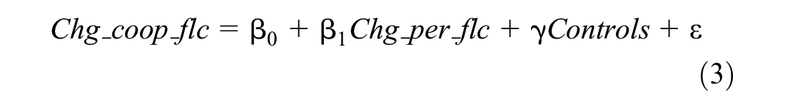
Chg_coop_flc = β_{0} + β_{1} Chg_per_flc + γ Controls + ε

(3)

where Chg_coop_flc represents the change of cooperation in the last year of last contract, that is, the difference between the assists rate (adjusted by position) in the last year and the assists rate (adjusted by position) in the year before last year of last contract. Chg_per_flc is the change of efficiency in the last year of last contract, that is, the difference between last year efficiency and the year before last year efficiency of last contract.

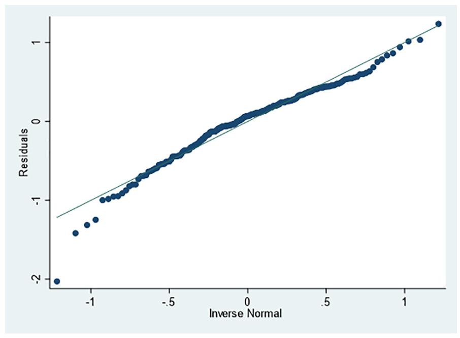
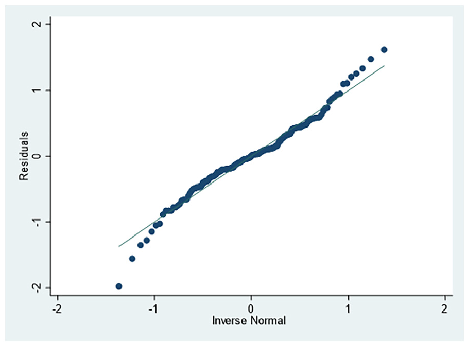
We run ordinary least squares (OLS) regression with robust standard errors adjusted heteroscedasticity for Model (3). Figure 3 shows the distribution of residual. From Figure 3 we can see that the skewness and kurtosis of residual are normal. Table 5 shows the regression results. Except for Age_flc and Age_squ_flc, the variance inflation factors (VIF) of other variables are less than 5. Column 1 represents that the coefficient of Chg_per_flc is positive and significant at the 1% level, which indicates that there is a positive relationship between the change of players’ efficiency and the change of players’ collaboration with team members. That is, the higher the player’s efficiency is, the more his cooperation with his teammates will be. This means that the player does not sacrifice the interests of the team in pursuit of personal efficiency in the last year based on the previous contract. Therefore, the hypothesis of “fake efficiency” is not valid. Column 2 presents the first robust test result. Chg_coop2_flc is the difference between the number of assists (adjusted by position) in the last year and the number of assists (adjusted by position) in the year before the last year of last contract. Similarly, the coefficient of Chg_per_flc is positive and significant at the 1% level, showing that players’ cooperation in t−1 year increases with their increased efficiency. That is to say, players cannot beautify their efficiency data at the expense of the team’s benefit. This result excludes the hypothesis of players’ fake efficiency. Column 3 shows the second robust test result. PER may contain assist information. To alleviate this effect, we first regress Chg_per_flc on Assist (the number of assists per game). Then we use the regression residual to replace Chg_per_flc and run regression as Model (3). The result shows that the coefficient of Chg_per_flc is positive and significant at the 1% level, consistent with column 1 and 2.

Figure 3.

The distribution of regression residual of Model (3).

Table 5.

Regression Results of the Change of Player’s Collaboration With Team Members on the Change of Player’s Efficiency.

	(1)	(2)	(3)
	Chg_coop_flc	Chg_coop2_flc	Chg_coop_flc
Intercept	−3.315 (0.713)	4.513 (0.691)	−2.138 (0.815)
Chg_per_flc	0.058*** (0.000)	0.088*** (0.000)
Residual of regression of Chg_per_flc on Assist			0.053*** (0.000)
Height	0.013 (0.929)	0.186 (0.331)	0.012 (0.935)
Weight	−0.005* (0.077)	−0.010** (0.012)	−0.005* (0.062)
Age_flc	−0.127 (0.321)	−0.197 (0.258)	−0.136 (0.308)
Age_squ_flc	0.003 (0.249)	0.004 (0.212)	0.003 (0.239)
GSR_flc	0.231* (0.053)	0.618*** (0.000)	0.271** (0.025)
WP	0.121 (0.318)	0.183 (0.231)	0.117 (0.346)
Forward	−0.031 (0.762)	−0.043 (0.739)	−0.018 (0.862)
Guard	−0.152 (0.300)	−0.314 (0.142)	−0.123 (0.408)
SC_fcc	0.304 (0.563)	−0.069 (0.917)	0.252 (0.636)
N	173	173	173
R ²	.2412	.3489	.208
Adj. R²	.1944	.3087	.159
F	3.551	6.673	3.013

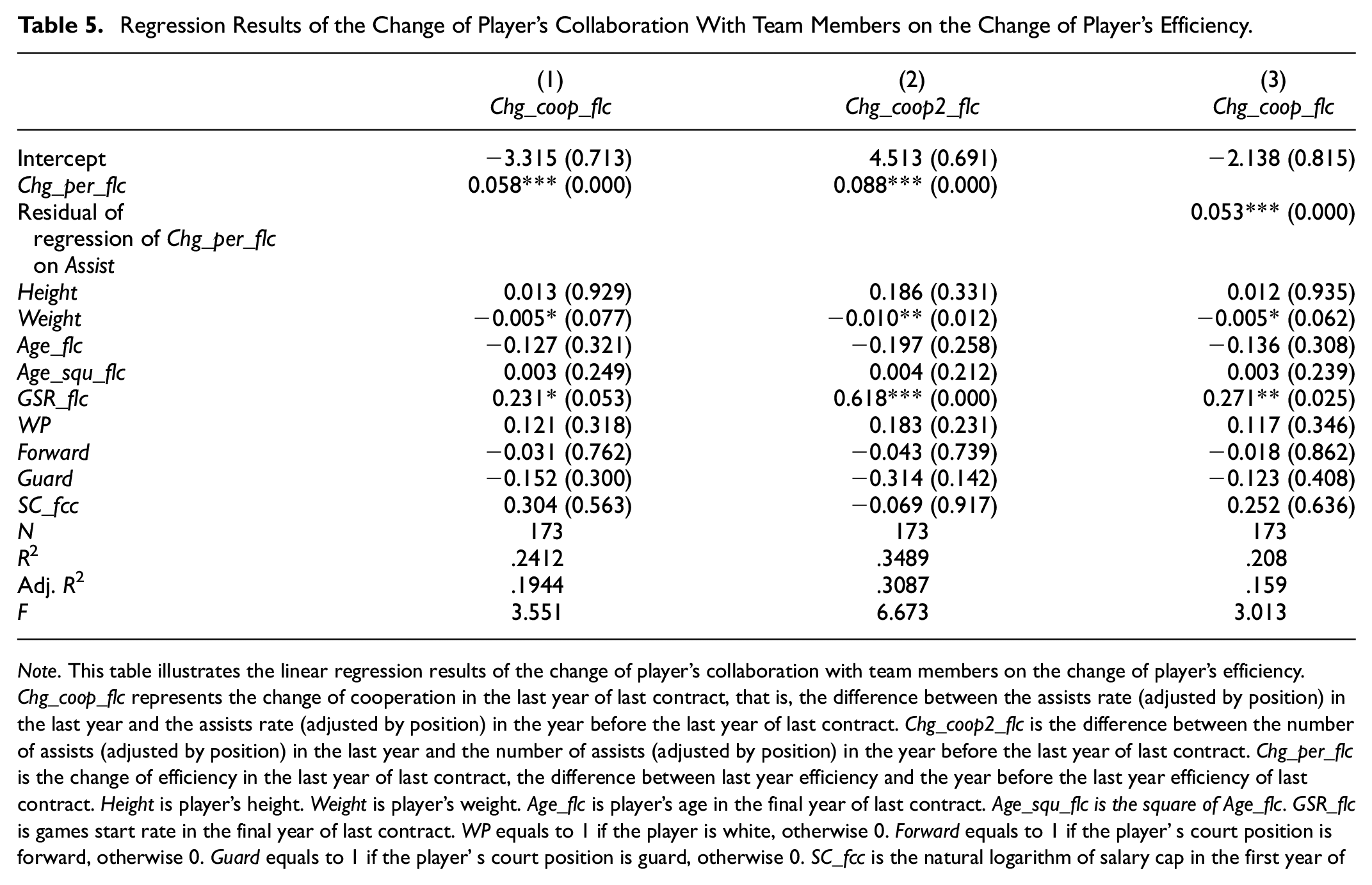
Note. This table illustrates the linear regression results of the change of player’s collaboration with team members on the change of player’s efficiency. Chg_coop_flc represents the change of cooperation in the last year of last contract, that is, the difference between the assists rate (adjusted by position) in the last year and the assists rate (adjusted by position) in the year before the last year of last contract. Chg_coop2_flc is the difference between the number of assists (adjusted by position) in the last year and the number of assists (adjusted by position) in the year before the last year of last contract. Chg_per_flc is the change of efficiency in the last year of last contract, the difference between last year efficiency and the year before the last year efficiency of last contract. Height is player’s height. Weight is player’s weight. Age_flc is player’s age in the final year of last contract. Age_squ_flc is the square of Age_flc. GSR_flc is games start rate in the final year of last contract. WP equals to 1 if the player is white, otherwise 0. Forward equals to 1 if the player’ s court position is forward, otherwise 0. Guard equals to 1 if the player’ s court position is guard, otherwise 0. SC_fcc is the natural logarithm of salary cap in the first year of current contract. p Value with standard errors adjusted heteroscedasticity in parentheses.

***

, **, and * are statistically significant at 1%, 5%, and 10% levels, respectively.

Secondly, is it because of managers’ myopia? That is, do managers make more weight on the players’ efficiency of t−1 year than on average efficiency of last contract? Before testing this hypothesis, our paper firstly compares the mean difference between the players’ efficiency of t−1 year and the efficiency of t−2 year of last contract. Because we cannot access to the duration data of last contract, what we can do is to compare the players’ efficiency of the last 2 years. As reported in Table 6, t value of paired t-test is positive and significant at the 1% level, which indicates that compared with the players’ efficiency in t−2 year of last contract, that in t−1 year significantly increases.

Table 6.

Mean Difference Between the Players’ Efficiency of t−1 year and the Efficiency of t−2 Year of Last Contract.

	PER
	Mean	Difference	t-Value
t−2 year of last contract	15.777	0.918**	2.486
t−1 year of last contract	16.695	0.918**	2.486

Note. This table compares the players’ efficiency of t−1 year with the efficiency oft−2 year of last contract.

is statistically significant at 5% level.

Furthermore, a regression model is constructed as follows.

\begin{matrix} Salary_fcc = & β_{0} + β_{1} Efficiency_flc + β_{2} Efficiency_alc \\ + γ Controls + ε \end{matrix}

(4)

where Efficiency_alc is the average efficiency for the last 2 years of the previous contract.

We run ordinary least squares (OLS) regression with robust standard errors adjusted heteroscedasticity for Model (4). Figure 4 shows the distribution of residual. From Figure 4 we can see that the skewness and kurtosis of residual are normal. Table 7 represents the regression results. Except for Age_flc and Age_squ_flc, the variance inflation factors (VIF) of other variables are less than 5. Column 1 shows that Efficiency_flc is positive and significant at the 1% level, while Efficiency_alc is not significant, which indicates that managers may put more weight on the players’ efficiency of t−1 year than on the average efficiency of last 2 years of last contract. This finding supports the hypothesis of managers’ myopia. Column 2 shows the first robust test. Because Efficiency_alc may contain information of Efficiency_flc, we first run regression of Efficiency_alc on Efficiency_flc. Then we use the residual to replace Efficiency_alc and run regression of Model (4). The result in column 2 shows that the coefficient of Efficiency_flc is positive and significant at the 1% level, while the coefficient of the residual of regression of Efficiency_alc on Efficiency_flc is not significant. Column 3 shows the second robust test. We test the effect of efficiency in t−2 years on Salary_fcc. The result shows that the coefficient of efficiency in t−2 year is not significant, indicating that not enough attention has been paid to efficiency in the year before last year of last contract when managers design players’ salary contracts. Because we cannot access to the duration data of last contract, we cannot construct an indicator of the average efficiency of the last whole contract. However, if managers do not put their attention on the last 2 years of last contract, they have lower incentive to focus on the average efficiency of the last whole contract. Therefore, Efficiency_alc can explain managers’ myopia.

Figure 4.

The distribution of regression residual of Model (4).

Table 7.

Regression Results of the First-Year Salary of Current Contract on the Efficiency of First Year of Current Contract and the Efficiency of the Average Last 2 Years of Last Contract.

	(1) Salary_fcc	(2) Salary_fcc	(3) Salary_fcc
Intercept	−14.864 (0.121)	−14.801 (0.123)	−15.228 (0.149)
Efficiency_flc	0.064*** (0.000)	0.073*** (0.000)
Efficiency_alc	0.014 (0.464)
Residual of regression of Efficiency_alc on Efficiency_flc		0.014 (0.464)
Efficiency in t–2 year			0.015 (0.163)
Salary_flc	0.235*** (0.003)	0.235*** (0.003)	0.372*** (0.000)
Height	0.016 (0.910)	0.016 (0.910)	−0.069 (0.655)
Weight	0.001 (0.531)	0.001 (0.531)	0.003 (0.319)
Age_flc	0.372*** (0.001)	0.372*** (0.001)	0.231* (0.071)
Age_squ_flc	−0.007*** (0.000)	−0.007*** (0.000)	−0.005** (0.023)
GSR_flc	0.400*** (0.003)	0.400*** (0.003)	0.497*** (0.001)
WP	0.070 (0.495)	0.070 (0.495)	0.003 (0.982)
Forward	−0.101 (0.214)	−0.101 (0.214)	−0.106 (0.249)
Guard	0.148 (0.259)	0.148 (0.259)	0.127 (0.424)
SC_fcc	1.115** (0.023)	1.115** (0.023)	1.203** (0.029)
N	173	173	173
R ²	.5837	.5837	.4940
Adj. R²	.5525	.5525	.4594
F	21.576	21.576	15.986

Note. This table describes the linear regression results of the first-year salary of current contract on the efficiency of first year of current contract and the efficiency of the average last 2 years of last contract. Salary_fcc is the natural logarithm of players’ salaries in the first year of current contract. Efficiency_flc is the PER in the final year of last contract. Efficiency_alc is the average efficiency for the last 2 years of the previous contract. Salary_flc is the natural logarithm of players’ salaries in the final year of last contract. Height is the player’s height. Weight is the player’s weight. Age_flc is the player’s age in the final year of last contract. Age_squ_flc is the square of Age_flc. GSR_flc is games start rate in the final year of last contract. WP equals to 1 if the player is white, otherwise 0. Forward equals to 1 if the player’ s court position is forward, otherwise 0. Guard equals to 1 if the player’ s court position is guard, otherwise 0. SC_fcc is the natural logarithm of salary cap in the first year of current contract. P value with standard errors adjusted heteroscedasticity in parentheses.

***

, **, and * are statistically significant at 1%, 5%, and 10% levels, respectively.

Results and Discussion

A good compensate contract is a useful method for a manager to motivate employees. Different from previous studies, this paper provides empirical evidences of the impact of an employee’s pre-contract efficiency on his/her salary and whether this pay decision is necessarily correct and provides some reasons.

Our article addresses the following three issues. First, are managers’ pay decisions based on pre-contract efficiency? Second, are these decisions correct? Third, if the decisions are not correct, why? We use data of National Basketball Association (NBA) players’ salary contracts to test the above questions. The empirical results show that how much managers pay their employees is indeed based on pre-contract efficiency. However, the pay decisions are not correct because relative to the final year of last contract (t−1 year), players’ efficiency in the first year of current contract (t year) decreases with increased salaries.

Why does this phenomenon happen? Our findings show that players’ collaboration in t−1 year increases with their increased efficiency, which indicates that players’ increased personal efficiency is not detrimental to the team’s performance, that is to say, players cannot inflate their efficiency data at the expense of the team’s performance. This result excludes the hypothesis of players’ fake efficiency. Furthermore, we do find that managers put weight on the players’ efficiency of t−1 year instead of on the average efficiency of last contract. This finding supports the hypothesis of managers’ myopia.

Our article may have certain innovations. Firstly, different from prior studies, we use each player’s contract as an observation sample, which guarantees the reliability of the conclusion. Secondly, this study increases our understanding of the mechanism of determining salary. Our study not only finds that managers’ decisions on employees’ salaries are not correct, but also explores the reasons and finds that managers only consider the players’ efficiency in t−1 year. Therefore, our study enriches literature of salary determinants.

These findings have some implications. On the one hand, when managers determine players’ salaries, it may be wiser to put more weight on the players’ average efficiency instead of the last year efficiency of last contract. On the other hand, in terms of operation management, NBA teams operate in a manner which is similar to that of corporations. From the perspective of employers within NBA teams, players are the core assets of teams, which is similar to the situation in the high-tech firms where technical personnel are the core assets of the corporation. Accordingly, the conclusions of this study can be applied to corporations.

Something broader to consider is that other indicators besides PER may be used to evaluate players. Besides, further study may be interesting on the other assess methods of cooperation and the substantial impact of how the team play offensively and defensively. In addition, future research in this area can cover several other variables in different sports and different regimes.

Footnotes

Appendix A

Declaration of Conflicting Interests

The author(s) declared no potential conflicts of interest with respect to the research, authorship, and/or publication of this article.

Funding

The author(s) disclosed receipt of the following financial support for the research, authorship, and/or publication of this article: This work was supported by Shantou University Scientific Research Initiation Grant [STF19011]; Guangdong Province University Characteristic Innovation Project [2019WTSCX029]; Philosophy and Social Science Foundation of Guangdong Planning Office [GD20XYJ39]; the National Natural Science Foundation of China [71702161]; Zhejiang Provincial Natural Science Foundation of China [17G020008LQ]; Zhejiang Philosophy and Social Science Planning Project [16NDJC021Z]; and the Zhejiang University of Finance and Economics research and innovation team.

ORCID iD

Riguang Wen

References

Balsam

Gifford

R. H.

Puthenpurackal

(2017). Related party transactions, corporate governance and CEO compensation. Journal of Business Finance & Accounting, 44, 854–894.

Berri

D. J.

Krautmann

A. C.

(2006). Shirking on the court: Testing for the incentive effects of guaranteed pay. Economic Inquiry, 44(3), 536–546.

Bodvarsson

O. B.

Brastow

R. T.

(1998). Do employers pay for consistent performance? Evidence from the NBA. Economic Inquiry, 36, 145–160.

Bryan

Nash

Patel

(2015). The effect of cultural distance on contracting decisions: The case of executive compensation. Journal of Corporate Finance, 33, 180–195.

Caglio

Dossi

Van der Stede

W. A.

(2018). CFO role and CFO compensation: An empirical analysis of their implications. Journal of Accounting and Public Policy, 37, 265–281.

Callan

S. J.

Thomas

J. M.

(2014). Relating CEO compensation to social performance and financial performance: Does the measure of compensation matter? Corporate Social Responsibility and Environmental Management, 21, 202–227.

Compton

Y. L.

Gore

A. K.

Kulp

S. L.

(2017). Compensation design and political risk: The case of city managers. Review of Accounting Studies, 22, 109–140.

Cordeiro

J. J.

Conyon

Shaw

T. S.

(2013). Informativeness of performance measures and Chinese executive compensation. Asia Pacific Journal of Management, 30, 1031–1058.

GarcíaMeca

(2016). Political connections, gender diversity and compensation policy. Review of Managerial Science, 10, 553–576.

10.

Grund

Walter

(2015). Management compensation and the economic crisis: longitudinal evidence from the German chemical sector. Review of Managerial Science, 9, 751–777.

11.

Harder

J. W.

(1992). Play for pay effects of inequity in a pay-for-performance context. Administrative Science Quarterly, 37, 321–335.

12.

Harkin

S. M.

Mare

D. S.

Crook

J. N.

(2019). Average pay in banks: do agency problems and bank performance matter? Review of Quantitative Finance and Accounting, 53, 101–122.

13.

Inoue

Plehn-Dujowich

J. M.

Kent

Swanson

(2013). Roles of performance and human capital in college football coaches’ compensation. Journal of Sport Management, 27, 73–83.

14.

Liang

Renneboog

Sun

S. L.

(2015). The political determinants of executive compensation: Evidence from an emerging economy. Emerging Markets Review, 25, 69–91.

15.

Luo

(2015). CEO power, ownership structure and pay performance in Chinese banking. Journal of Economics and Business, 82, 3–16.

16.

Paulsen

R. J.

(2021). New evidence in the study of shirking in Major League Baseball. Journal of Sport Management, 35, 285–294.

17.

Scott

1. A.

Long

1. E.

Somppi

. (1985). Salary vs. marginal revenue product under monopsony and competition: The case of professional basketball. Atlantic Economic Journal, 13, 50–59.

18.

Scully

G. W.

(1974). Pay and performance in major league baseball. The American Economic Review, 64, 915–930.

19.

Soebbing

B. P.

Wicker

Watanabe

N. M.

(2016). The effects of performance expectations on total compensation of Division I–Football Bowl Subdivision head coaches. Journal of Sport Management, 30, 70–81.

20.

Solow

J. L.

Krautmann

A. C.

(2020). Do you get what you pay for? Salary and ex ante player value in Major League Baseball. Journal of Sports Economics, 21, 705–722.

21.

Stiroh

K. J.

(2007). Playing for keeps: Pay and performance in the NBA. Economic Inquiry, 45, 145–161.

22.

van Essen

Otten

Carberry

E. J

. (2015). Assessing managerial power theory: Ameta-analytic approach to understanding the determinants of CEO compensation. Journal of Management, 41, 164–202.

23.

Wallace

(1988). Labor market structure and salary determination among professional basketball players. Work and Occupations, 15, 294–312.