Sage Journals: Discover world-class research

Abstract

The government of Ghana and the National Insurance Commission have shown concern over the low insurance patronage in Ghana. In order to take the necessary steps to increase insurance patronage, there is the need to, among other things, find the macroeconomic determinants of insurance demand in Ghana. The purpose of this study is to model the macroeconomic and demographic determinants of life insurance demand in Ghana. Data covering the period 1994 through 2020 are used for the study. Even though many studies have been done on determinants of insurance demand elsewhere (not in Ghana), almost all these studies use ordinary least square regression, stepwise regression, or similar regression methods. However, these methods are not robust enough to handle problems of multicollinearity, over-fitting, and inability to do out-of-sample prediction. This current study uses a regularization method known as elastic net regression algorithm which is more robust for handling the aforementioned problems, and more. The results of the study show that the dominating predictors (those with non-zero coefficients) of life insurance demand include old aged dependency ratio, life expectancy, urbanization, and financial development. The first three have positive relation with life insurance demand, while the last one has negative relation with life insurance demand. Insurance regulators and insurance companies are advised to design more innovative and attractive insurance policies for the aged and the old aged dependents as they have the highest tendency to affect insurance demand in Ghana.

Keywords

life insurance insurance demand insurance penetration insurance density elastic net regression

Introduction

The Government of Ghana and the National Insurance Commission (NIC; the regulator of the insurance industry of Ghana) have been expressing concern over the relatively low insurance penetration in Ghana. While the insurance penetration of South Africa for instance was about 12.70 % in 2008, that of Ghana for the same year was about 1.57%. In 2010, the insurance penetration of South Africa increased to 14.8%; but that of Ghana was at 1.89%. In 2019, the insurance penetration in Ghana declined to approximately 1% (NIC, 2019). The Government of Ghana has recently tasked the NIC to take steps to ensure that there is vibrancy in the insurance industry to increase insurance demand in Ghana (Ghanaweb, 2019). This calls for studies into the country-specific macroeconomic and demographic factors that affect insurance demand in Ghana, in order to effectively remedy the problem of low insurance demand in Ghana.

Factors affecting insurance demand have been studied extensively in literature; and these studies take either of two main perspectives (Zerriaa et al., 2017). According to Zerriaa et al. (2017), the studies are either based on microeconomic survey data on households, to test theoretical conclusions derived from the life-cycle and permanent income hypothesis; or they are based on macroeconomic cross-sectional, panel, or single-country data. To the best of our knowledge, almost all the country-specific (or single-country) studies on the determinants of insurance demand in Ghana take the former perspective, whereby the studies involve the collection of microeconomic survey data on households (Ampaw et al., 2018; Fofie, 2016; Peprah et al., 2017). Studies taking the latter perspective which involves the use of macroeconomic data, are lacking in Ghana. However, considering government’s interest in increasing insurance demand in Ghana as a sovereignty, it is necessary that country-specific, macroeconomic perspective is taken to study the determinants of insurance demand in Ghana. Knowing the macroeconomic (and demographic) determinants of insurance in Ghana would help government identify the roles it can also play to effectively resolve the problem of low insurance demand. Such information can also provide insights for other governments in promoting insurance business globally. Similar studies have been done for many countries, including Tunisia, China, and Canada (Mapharing et al., 2015; Yuan & Jiang, 2015; Zerriaa et al., 2017).

Usually, the most popular regression method used in modeling insurance determinants is the Ordinary Least Squared or OLS (or other similar methods). Due to the potential multicollinear nature of the predictors sometimes, some other studies make use of variable selection or dimension reduction methods, such as stepwise regression, block wise regression, backward elimination, or forward selection. However, “a fundamental problem with stepwise regression [and similar methods] is that some real explanatory variables that have causal effects on the dependent variable may happen to not be statistically significant, while nuisance variables may be coincidentally significant. As a result, the model may fit the data well in-sample, but do poorly out-of-sample” (Smith, 2018, p.1). More advanced machine learning algorithms have been developed to remedy the limitations of the OLS and the stepwise regression, in dealing with multicollinearity among predictors. One of such methods is the elastic net regression. This current study aims at using the elastic net to model the demand for life insurance, considering the potential multicollinearity between the predictors. To the best of our knowledge, this is the first study to model the demand for life insurance using the elastic net regression.

The remaining of the work is organized as follows. Section 2 discusses regularization and how it helps in dealing with multicollinearity; section 3 discusses literature review on the determinants of life insurance demand; section 4 discuses data and methodology; section 5 discusses results and analysis; and section 6 gives conclusion, policy implication, and recommendations.

Multicollinearity and Regularization

Machine learning algorithms are continuously attracting attention in the research community, across almost all disciplines. In fact, studies in the areas of economics and econometrics are not exempted (Athey, 2017; Kleinberg et al., 2018; Mullainathan & Spiess, 2017; Varian, 2014). One of the machine learning applications relevant in economic research is regularized regression, or regularization. Regularization does not only minimize the sum of squared deviations between observed and model-predicted values, but in addition imposes a regularization penalty which limits the complexity of the model.

When multicollinearity is present between predictors, the ordinary least squares (OLS) estimates can give inaccurate predictions when used for multiple linear regression models. Although OLS estimates are unbiased, they can result in highly variable predictions (increased variance) when no variable selection is performed. In fact, in the presence of multicollinearity, the OLS estimator yields regression coefficients whose absolute values are too large and whose signs may actually reverse with negligible changes in the data (Buonaccorsi, 1996). One way to improve the predictions is to reduce the number of variables in the model by feature selection. Therefore, in attempt to reduce the effects of multicollinearity, some studies use stepwise regression, backward elimination, forward selection, blockwise selection, and other similar stepwise regression algorithms. For instance, in studying the factors affecting life insurance demand in Tunisa, Zerriaa et al. (2017) used the stepwise regression method to remedy collinearity between the predictors.

However, these stepwise regression methods tend to drop predictors entirely even though they may be relevant in predicting the response variables. Again, the coefficients may still be sensitive to the slightest addition or dropping of predictors in the model. According to Smith (2018), “a fundamental problem with stepwise regression is that some real explanatory variables that have causal effects on the dependent variable may happen to not be statistically significant, while nuisance variables may be coincidentally significant. As a result, the model may fit the data well in-sample, but do poorly out-of-sample” (Smith, 2018, p.1).

A class of alternative parameter estimation algorithms known as regularization, or shrinkage techniques have been proven to perform better than the stepwise regression methods (Finch & Finch, 2016). According to Finch and Finch (2016), whereas feature selection methods such at the stepwise regression assign an inclusion weight of either 1 or 0 (either include or exclude a variable in the model), and subsequently estimate the value of coefficients for the independent variables included in the model, regularization methods first of all estimate optimal values of coefficients of all the predictors in the model, such that the most important variables receive higher values, and the least important are assigned coefficients at or near 0. That is, unimportant variables may subsequently be assigned zero value only after the optimization, which results in such variables excluded from the model. Consequently, the resulting regularized model’s variances and standard errors do not suffer from the type of inflation common with stepwise regression models and other similar feature selection methods. The main examples of the regularization methods are the ridge regression, LASSO (least absolute shrinkage and selection operator) regression, and the elastic net regression.

The method of ridge regression, proposed by Hoerl and Kennard (1970), is one of the most widely used tools to treat the problem of multicollinearity. In ridge regression, an additional parameter, the ridge parameter, plays an important role to control the bias of the regression toward the mean of the response variable, by shrinking the coefficients of the explanatory variables (Dorugade, 2014). However, the ridge regression does not shrink any coefficient completely to zero, irrespective of how small the coefficient value remaining. Therefore it does not lead to the dropping of any of the predictors entirely from the model, irrespective of how irrelevant the predictors might be (in predicting the response variables).

To solve the deficiencies of classical linear model selection methods (such as the stepwise regression), as well as to amend the limitation of the ridge regression, Tibshirani (1996) developed the least absolute shrinkage and selection operator (LASSO), which selects variables and estimates parameters simultaneously. Unlike stepwise model selection, LASSO uses a tuning parameter (the LASSO parameter or lambda) to penalize the number of parameters in the model. Complicated iterative process is used to choose the value of the lambda. This is done with cross-validation so as to minimize the Mean Squared Error (MSE) of the prediction. Moreover, while traditional regression techniques are limited in the analysis and synthesis of large numbers of covariates, LASSO methodology permits for a large number of covariates in the model. In addition, LASSO, has the unique feature of penalizing the absolute value of a regression coefficient; thus, regulating the impact a coefficient may have on the overall regression. The greater the penalization, the greater the shrinkage of coefficients, with some reaching zero. Thus, automatically removing unnecessary/uninfluential covariates. The major limitation of LASSO is that its variable selection can be too dependent on data and thus unstable.

To obtain the strengths of both LASSO and ridge regression, Zou and Hastie (2005) proposed the elastic net regression, which is a combination of the LASSO and ridge regressions. The elastic net is to combine the penalties of ridge regression and LASSO to get the best of both algorithms. Zou and Hastie (2005) prove that the elastic net outperforms the LASSO, while enjoying a similar sparsity of representation. In addition, the elastic net encourages a grouping effect, where strongly correlated predictors tend to be in or out of the model together. The elastic net is particularly useful when the number of predictors (p) is much bigger than the number of observations (n). This makes elastic net suitable in situations where there is limited number of observations in the dataset (small samples) as usually experienced in most African countries, including Ghana. Therefore this study uses the elastic net regression to model the demand for life insurance in Ghana, using predictors which may potentially be collinear. The elastic net is used to estimate the optimum values of coefficients and simultaneously eliminate the predictors which are irrelevant in the model. The cross-validation procedure is used to estimate the optimum parameters that minimize the mean squared error.

Literature Review

Life Insurance Demand

The purpose of our study is to model the demand for life insurance, and to identify the factors which contribute to life insurance demand in Ghana. We use both insurance density and insurance penetration as proxy for insurance demand. In literature, both are used as alternatives to represent insurance demand (Zhang & Zhu, 2005). Insurance density is the premium per capita and it relates more to insurance consumption or patronage. In other words, insurance density signifies insurance demand by the people. Insurance penetration on the other hand, is the premium as a percentage of GDP and it relates more to the extent to which insurance contributes to GDP or economic development. In other words, insurance penetration signifies insurance industry development. Park and Lemaire (2012) explain that penetration measures insurance consumption relative to the size of the economy, while density measures insurance purchases per individual. Beck and Webb (2003) emphasizes that insurance density is more income elastic than insurance penetration. Although the two concepts have slightly different interpretations, their determinants (predictors) are almost always the same in literature.

Determinants of Life Insurance Demand

Income

With respect to macroeconomic determinants of insurance, most studies show that income per capita, which measures the economic development level of a country, is the most important. Income has been found to be the most important probably because it leads to affordability and ultimately higher demand for insurance products (Browne & Kim, 1993; Hammond et al., 1967). Beck and Webb (2003) assert that rise in income leads to rise in human capital which ultimately increases life insurance product demand. Ćurak and Gašpić (2011) in their study also find that income is positively associated with demand for life insurance. Studies by Browne and Kim (1993) and Outreville (1996) have shown that life insurance development is positively influenced by income. Demand for life insurance is positively correlated with income not only because life insurance becomes more affordable as income increases, but also because the need for life insurance increases with income as it protects dependents against the loss of expected future income due to premature death of the main income earner (Browne & Kim, 1993). Guerineau and Sawadogo (2015) also add that income is an essential variable in the life insurance consumption as this is justified by the necessity to ensure maintained income level for dependents

Even though many studies have shown that the effect of income on insurance is very significant, some of such studies add conditions that the effect depends on the economic development level of the country in question. Truett and Truett (1990) in their study compare the life insurance demands in Mexico and United States, and find that the income elasticity of life insurance consumption is higher in Mexico than in the United States. Enz (2000) in his study identifies the factors of demand and supply that are likely to influence life insurance penetration in 90 countries. The results show that the income elasticity of life insurance penetration is not constant across countries. It is also noted that there is a level of per-capita income at which the income elasticity of demand for insurance reaches a maximum. Moreover, there appears to be lower and upper limits to the amounts of income that can be spent on insurance. This relation between income and insurance demand is termed as the so-called S-curve (Enz, 2000). Finally, Feyen et al. (2011) also confirm that the effect on life insurance consumption generally varies with the income level. They further opine that the very wealthy groups of individuals may not need the life insurance because they think they have excess financial resources, while the very poor people may also not have the means to purchase life insurance products.

Inflation

Inflation is among the factors found to affect the demand for insurance. Greene (1954) and Babbel (1981) have shown that inflationary expectations have a significant negative impact on life insurance consumption. Beck and Webb (2003) also find that inflation negatively influences insurance consumption in both developed and developing countries. First of all, it is expected that inflation (and its volatility) would have negative relationship with life insurance consumption. This is because the inflation reduces the purchasing power of the savings aspect of life insurance. Secondly, inflation can also have a disruptive effect on the life insurance industry when interest rate cycles spur disintermediation. These dynamics make inflation an additional encumbrance to the product pricing decisions of life insurers, thus, possibly reducing supply in times of high inflation (Beck & Webb, 2003). Inflation erodes the value of life insurance, making it a less desirable good. Consequently, in an effort to mitigate the life insurance value erosion produced by inflation, insurers in many countries offer indexed life insurance policies whose face values are adjusted by some price index over time (Browne & Kim, 1993). However, Babbel (1981) shows that even the demand for indexed life insurance is reduced during inflationary periods. This is because of the fact that the death benefit of an indexed life insurance policy is typically adjusted only at the beginning of each year, to recover the value lost due to inflation during the previous year. Hence the real value of life insurance is reduced if an insured dies during a year of high inflation.

While many studies find negative relationship between inflation and insurance consumption, Hwang and Gao (2003) on the contrary find that insurance demand, in the case of China, is not adversely affected by higher inflation. They explain that during higher inflationary period, higher economic growth could occur. So people would be less reactive toward insurance consumption during higher inflation.

Financial Development

Iyawe and Osamwonyi (2017) show that financial development in African countries drives life insurance demand more than major macroeconomic factors. Beck and Webb (2003) argue that a good banking sector (or developed financial system) increases the confidence consumers have in their financial institutions (including insurers). Furthermore, to provide some form of guarantee to protect loans from financial institutions, clients are required to purchase life insurance policies to serve as security against the events whereby it might become impossible for borrowers to repay their debts, either due to incapacitation or death. Hence developed financial sector potentially contributes to life insurance demand.

Education

Truett and Truett (1990) and Browne and Kim (1993) find a positive relationship between life insurance consumption and level of schooling. It is perceived that a higher level of education increases the ability of clients to understand the benefits of risk management and long-term savings (in the form of life insurance). Curak et al. (2013) also suggest that education increases risk aversion and encourages people to demand life insurance. Treerattanapun (2011) also states that education increases the awareness of risk and threats to financial stability, facilitating the understanding of insurance benefits.

Education may also increase the value of human capital of the primary wage earner, hence the need to be protected through insurance. Also, education lengthens the period of dependency; therefore, when individuals are educated over a longer time period, there would be a higher demand for life insurance for the one who is being depended on (Browne and Kim (1993). Furthermore, when the level of the educated population increases in a country, the recognition of the available life insurance products increases, and this leads to higher demand for life insurance. Positive relation between education and life insurance might also be explained by the fact that better access to long-term savings and insurance instruments encourages access to higher education.

Interestingly, Beck and Webb (2003) show that school enrollment rate (education) does not have strong link with the life insurance consumption in 68 countries from 1960 to 2000. Feyen et al. (2011) also discover that even though individuals with higher education generally have higher incomes and tend to purchase life insurance, schooling does not seem to be an important driver of life insurance. Interestingly, at the very extreme end, Duker (1969), Anderson and Nevin (1975), and Auerbach and Kotlikoff (1989) reveal that education is negatively related to life insurance demand.

Dependency Ratio

Dependency ratio is considered another important factor affecting insurance consumption. Dependency ratio is defined by Lenten and Rulli (2006) as average family members dependent on a primary income earner for a living. Dependency ratio can be divided into two: old aged dependency ratio and young aged dependency ratio. Old aged dependency ratio is defined as the ratio of dependents over 64 years, divided by working age population aged 15 through 64 years. Young aged dependency ratio is defined as ratio of dependents under age 15 years, divided by working age population aged 15 through 64 years. A basic driving force for demand for insurance is the tendency to provide protection from financial hardships to one’s dependents (Lewis, 1989; Li et al., 2007). The proceeds from life insurance claims would compensate for income loss to dependents upon the demise of a bread winner, and this serves as one of the major reasons for the purchase of life insurance (Hammond et al., 1967). Lewis (1989) show that the demand for life insurance increases with the number of dependents in a household. Redzuan (2014) also find positive impact of number of dependents on life insurance in Malaysia.

While some studies find high dependency ratio to have a positive relationship with life insurance consumption, Beck and Webb (2003) find the relationship not to be consistent across both developed and developing countries. Moreover, they find an ambiguous relationship for young dependency ratio (dependents below age 15 years) and a positive relationship for old dependency ratio (dependents above age 64 years). Meanwhile, some other studies provide evidence that young dependency ratio causes a decline in life insurance demand for saving motive (Beck & Webb, 2003; Sen, 2008; Sen & Madheswaran, 2007). For primary wage earners, larger family size can be a burden on financial resources, thereby reducing demand for insurance (Akhter & Khan, 2017). Alhassan and Biekpe (2016) find dependency ratio to lead to decline in life insurance consumption in Africa. They argue that high dependency ratio serves as strain on income due to high levels of current expenditure, hence individuals would not have enough left of their income to purchase life insurance.

Life Expectancy

Life expectancy is the average number of years the average individual in a country is expected to live. Outreville (1996) find positive influence of life expectancy on life insurance. Sulaiman et al. (2015) in their study investigate the variables that influence life insurance demand in Ethiopia from 1980 to 2008. They find that life expectancy is positively associated with life insurance. On the contrary, Li et al. (2007) find a negative relationship between life expectancy and life insurance. Alhassan and Biekpe (2016) also find life expectancy to lead to decline in life insurance consumption in Africa.

Meanwhile Browne and Kim (1993) find that life expectancy is not an important factor of life insurance consumption. This is supported by Beck and Webb (2003) who show that life expectancy does not have strong link with the life insurance consumption in 68 countries from 1960 to 2000. They clarify that even though societies with longer life expectancies are expected to have lower need for mortality coverage, they might need higher savings through life insurance vehicles and more demand for annuities. This therefore implies an ambiguous correlation of life expectancy with the demand for life insurance products (Beck & Webb, 2003).

Savings

Schwebler (1984) and Beck and Webb (2003) show significant positive effect of savings on life insurance demand. Zhang and Zhu (2005) also find significant positive impact of savings on life insurance premiums. On the other hand, life insurance policies can be regarded as savings products, and therefore the premiums paid can be seen as alternative to saving at the bank. In other words, treating life insurance policies as one of several assets investors can choose from, makes life insurance an alternative to, or competing with savings at the bank. This means that a higher savings at the bank could negatively correlate with the purchase of life insurance. As opined by Feyen et al. (2011), the very wealthy groups of individuals may not need the life insurance because they think they have excess financial resources (at the bank).

Urbanization

Another important factor for the development of the insurance industry is urbanization (Akhter & Khan, 2017; Kalra et al., 2013). Urbanization comes along with industrialization and expansion of cities and towns. Urbanization, or more precisely the degree of urbanization, is defined as the percentage of population living in areas under the administration of a city or a town. Urbanization reflects the gradual shift from rural or farming based economies to industrialized economies. Economies with a higher share of urban to total population are expected to have higher levels of life insurance consumption. In other words, the development of life insurance is positively related to a country’s urbanization status (Sen, 2008; Sen & Madheswaran, 2007). Zerriaa et al. (2017) study the determinants of life insurance demand in Tunisia and they find that high level of urbanization stimulates life insurance demand in Tunisia. Hwang and Gao (2003) add that there is a positive impact of urbanization on saving propensity of urban people (through life insurance). They argue that insurance can play a vital role in providing protection and financial security to small families (which are usually found in urban areas).

Furthermore, the concentration of consumers in a geographic area usually simplifies the task of distributing life insurance products. The costs related to marketing, premium collection, underwriting, and claim handling are reduced. A higher degree of urbanization is hence likely to increase life insurance sales (Alhassan & Biekpe, 2016).

However, some other studies find urbanization as insignificant determinant of insurance consumption. Beck and Webb (2003) do not find significant impact of urbanization on life insurance demand. Nesterova (2008) also suggests that urbanization level is not significant for life insurance demand. On the face of the ambiguity of the impact of urbanization, a study by Dragos (2014) distinguishes that urbanization influences significantly the life insurance demand in Asia, but not in Europe. Interestingly, Alhassan and Biekpe (2016) find a negative effect of urbanization on life insurance in Africa, though the significance of the relationship is not robust.

Data and Methodology

The study seeks to find out the macroeconomic and demographic factors affecting the demand for life insurance in Ghana. The study uses data covering the period 1994 through 2020. This study period is chosen based on availability of relevant data. Based on the literature review, we use the following proxies and computations for variables used in the study.

Dependent Variable

We use insurance density and insurance penetration as proxies for insurance demand. Insurance density is calculated as the annual gross premium divided by the total population of the country. Insurance penetration is calculated as the annual gross premium as a percentage of annual GDP of the country. We obtain the gross premium from the annual reports of the National Insurance Commission, and obtain population and GDP from the World Bank’s database of economic indicators.

Independent Variables

Income

We use GDP per capita as proxy for income. This variable is obtained from the World Bank’s database of economic indicators.

Savings

We use bank deposit rate as a proxy for savings. If deposit rates are high, it is likely that people would save their monies at the bank or other similar deposit taking financial institutions. We obtain this variable from the World Bank’s database of economic indicators.

Education

We use tertiary school enrolment rate as a proxy for education. The variable is obtained from the World Bank’s database of economic indicators.

Inflation

We use change in consumer prices as proxy for inflation and this is obtained from the World Bank’s database of economic indicators.

Financial Development

We use domestic credit provided by financial institutions (as percentage of GDP) as proxy for financial development. The variable is obtained from the World Bank’s database of economic indicators.

Dependency Ratio (Old Dependents)

This ratio is defined as the ratio of dependents under age 15 years, divided by working age population aged 15 through 64 years. The variable is obtained from the World Bank’s database of economic indicators.

Dependency Ratio (Young Dependents)

This ratio is defined as the ratio of dependents over age 64 years, divided by working age population aged 15 through 64 years. The variable is obtained from the World Bank’s database of economic indicators.

Life Expectancy

This variable is obtained from the World Bank’s database of economic indicators.

Urbanization

We use urban population (as percentage of total population) as proxy for this variable. This variable is obtained from the World Bank’s database of economic indicators.

Model Specification

Based on literature, the following models are used to determine life insurance demand. Per definition, model 1 determines insurance development and model 2 determines insurance patronage.

Model 1

\begin{matrix} LIFEDEN = β_{0} + β_{1} INC + β_{2} SAV + β_{3} URB + β_{4} EDU \\ + β_{5} INF + β_{6} FD + β_{7} LEXP + β_{8} DEOLD \\ + β_{9} DEYOUNG \end{matrix}

(1)

Model 2

\begin{matrix} LIFEPEN = β_{0} + β_{1} INC + β_{2} SAV + β_{3} URB + β_{4} EDU \\ + β_{5} INF + β_{6} FD + β_{7} LEXP + β_{8} DEOLD + β_{9} DEYOUNG \end{matrix}

(2)

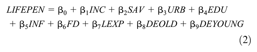
Where LIFEDEN = Life insurance density

LIFEPEN = Life insurance penetration

INC = Income

SAV = Savings (deposit interest rate)

URB = Urbanization

EDU = Education

INF = Inflation

FD = Financial development

LEXP = Life expectancy

DEOLD = Dependency ratio (old dependents)

DEYOUNG = Dependency ratio (young dependents)

Mathematical Formulation of the Regularization Problem

This formulation is adapted from The Mathworks (2021). When independent variables are correlated and the columns of the design matrix $X$ have an approximate linear dependence, the matrix $(X^{T} X)^{- 1}$ is close to singular. Therefore, the least-squares estimate $β = (X^{T} X)^{- 1} X^{T} y$ is highly sensitive to random errors in the observed response $y$ producing a large variance.

Ridge Regression

Ridge regression addresses the problem of multicollinearity by estimating regression coefficients using $β = (X^{T} X + λ I)^{- 1} X^{T} y$ . Where $λ$ is the ridge parameter and $I$ is the identity matrix. A small, nonnegative value of $λ$ can improve the conditioning of the problem and reduce the variance of the estimates. The reduced variance of ridge estimates results in a smaller mean squared error when compared to least-squares estimates. For a given value of $λ$ , a nonnegative parameter, ridge regression solves the problem

min_{β_{0} β} (\sum_{i = 1}^{N} {(y_{i} - β_{0} - x_{i}^{T} β)}^{2} + λ \sum_{j = 1}^{p} β_{j}^{2})

Where

$N$ is the number of observations.

$y_{i}$ is the response at observation $i$

$x_{i}$ is the data, a vector of length $p$ at observation $i$

$λ$ is a nonnegative regularization parameter.

The parameter $β_{0}$ is a scalar, and the parameter $β$ is a vector of length $p$ . The rigde problem involves the $L^{2}$ norm of $β$ .

LASSO Regression

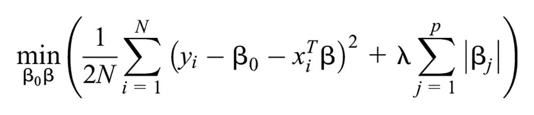
For a given value of the nonnegative parameter, $λ$ , LASSO regression solves the problem

min_{β_{0} β} (\frac{1}{2 N} \sum_{i = 1}^{N} {(y_{i} - β_{0} - x_{i}^{T} β)}^{2} + λ \sum_{j = 1}^{p} | β_{j} |)

As $λ$ increases, the number of nonzero components of $β$ decreases. The LASSO problem involves the $L^{1}$ norm of $β$ .

Elastic Net Regression

The elastic net solves the problem;

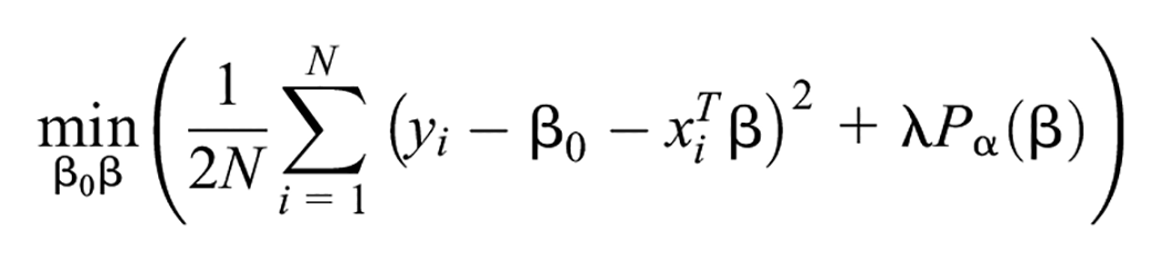
min_{β_{0} β} (\frac{1}{2 N} \sum_{i = 1}^{N} {(y_{i} - β_{0} - x_{i}^{T} β)}^{2} + λ P_{α} (β))

Where:

P_{α} (β) = \frac{(1 - α)}{2} ‖ β ‖_{2}^{2} + α ‖ β ‖_{1} = \sum_{j = 1}^{P} \frac{(1 - α)}{2} β_{j}^{2} + α | β_{j} |

(3)

Elastic net is the same as LASSO when α = 1, and the same as ridge regression when α shrinks to 0. For other values of α, the penalty term $P α (β)$ interpolates between LASSO and ridge regressions. That is, between the $L^{1}$ and the $L^{2}$ norms of $β$ . While the ridge regression proportionally shrinks the predictor coefficients to improve the out-of-sample prediction power of the model, the LASSO regression proportionally shrinks the coefficients, and in addition reduce to zero the coefficients of the predictors that contribute little to the model, thereby eliminating the respective irrelevant predictor(s). In our study, we are not only interested in the predictive power of the model, but also the relevance of the predictors. Hence we give marginally higher weight to LASSO than ridge, by setting $α$ to 0.6. However, the optimum $λ$ is determined through cross-validation processes of k = 10. The algorithm automatically standardizes the variables, does the optimization or estimation in the process, and then reconverts the results to reflect the original values.

Results and Discussion

Table 1 shows the summary statistics of the variables. As expected, young dependents are more than aged dependents in Ghana. The mean of young aged dependency ratio is 71.336 while that of the old aged dependency ratio is 5.142. This also implies that in Ghana, the population of the young is larger than that of the old aged. It is also shown that the average life expectancy of Ghanaians is 60 years. It ranges between 57 and 64 years.

Table 1.

Summary Statistics.

Variable	Obs.	Minimum	Maximum	Mean	Std. Deviation
LIFEDEN	27	0.14461	63.26220	12.8379633	18.22439340
LIFEPEN	27	0.00580	1.18424	0.2664067	0.34355772
INC	27	2492.31	5434.56	3660.9893	1003.16973
SAV	27	8.88542	35.75920	17.4175844	8.65278046
URB	27	39.390	57.349	48.59704	5.452211
EDU	27	0.69145	18.68750	7.9125789	6.33130855
INF	27	4.86540	59.46160	19.2744030	13.49549200
FD	27	5.07356	15.82750	12.0056919	3.04731599
LEXP	27	56.9720	64.4561	60.005485	2.5961367
DEPOLD	27	4.90363	5.35944	5.1423452	0.15062343
DEPYOUNG	27	62.1666	81.0963	71.336004	6.2695480

Note. LIFEDEN = life insurance density; LIFEPEN = life insurance penetration; INC = income; SAV = savings; URB = urbanization; EDU = education; INF = inflation; FD = financial development; LEXP = life expectancy; DEPOLD = old aged dependency ratio; DEPYOUNG = young age dependency ratio.

Table 2 shows the correlation matrix. Both dependent variables (life insurance density and life insurance penetration) have appreciable pairwise correlations with the independent variables. They have high correlation with income, urbanization, education, life expectancy, and young dependency ratio. They have moderate correlation with savings and inflation. Both life insurance density and penetration have negative correlation with savings, inflation, and young dependency ratio. This means that high savings has the tendency of decreasing life insurance demand. While life insurance density has positive correlation with old aged dependency ratio, life insurance penetration has negative relation with old aged dependency ratio.

Table 2.

Correlation Matrix.

	LIFEDEN	LIFEPEN	INC	SAV	URB	EDU	INF	FD	LEXP	DEPOLD	DEPYOUNG
LIFEDEN	1	0.9976	0.9064	−0.4298	0.8369	0.8677	−0.4162	0.0685	0.8821	0.0078	−0.8022
LIFEPEN	0.9976	1	0.9295	−0.4627	0.8659	0.8971	−0.4361	0.112	0.9095	−0.0405	−0.8352
INC	0.9064	0.9295	1	−0.6401	0.9665	0.9877	−0.5506	0.3485	0.9835	−0.3241	−0.9578
SAV	−0.4298	−0.4627	−0.6401	1	−0.7517	−0.6902	0.7003	−0.6379	−0.6785	0.7784	0.7832
URB	0.8369	0.8659	0.9665	−0.7517	1	0.974	−0.6212	0.5367	0.9625	−0.5024	−0.9944
EDU	0.8677	0.8971	0.9877	−0.6902	0.974	1	−0.5581	0.4139	0.9921	−0.4115	−0.9761
INF	−0.4162	−0.4361	−0.5506	0.7003	−0.6212	−0.5581	1	−0.5191	−0.541	0.4873	0.6192
FD	0.0685	0.112	0.3485	−0.6379	0.5367	0.4139	−0.5191	1	0.3539	−0.8007	−0.5483
LEXP	0.8821	0.9095	0.9835	−0.6785	0.9625	0.9921	−0.541	0.3539	1	−0.3974	−0.9682
DEPOLD	0.0078	−0.0405	−0.3241	0.7784	−0.5024	−0.4115	0.4873	−0.8007	−0.3974	1	0.5636
DEPYOUNG	−0.8022	−0.8352	−0.9578	0.7832	−0.9944	−0.9761	0.6192	−0.5483	−0.9682	0.5636	1

Paying closer attention to the independent variables, one can see that they have high pairwise correlations among themselves. Income for instance has high correlation with savings, urbanization, education, life expectancy, and old aged dependency ratio. Therefore, there is a potential problem of multicollinearity. As least squares estimation may not be appropriate for modeling multicollinear predictors, this study makes use of elastic net regression, which is very appropriate under the circumstance.

Figure 1a shows the trace plot of model 1 (which models life insurance density). Figure 1b shows same thing, but with legends. The elastic net algorithm shrinks the coefficients of the predictors to enhance the prediction power of the model. The more the lambda of the elastic net increases, the more the coefficients shrink. This leads to less variance, and hence makes the model more suitable for out-of-sample prediction.

Figure 1.

(a) Elastic net trace plot—life insurance density (without legends). (b) Elastic net trace plot—life insurance density (with legends).

The coefficients of the predictors in the model are all stable and less than 20, with the exception of old aged dependency ratio, which is dominating. Change in old aged dependency ratio has the highest effect on change in life insurance density. People tend to buy life insurance the more they have old aged dependents.

The green dotted line corresponds to the lambda at which the coefficients produce the minimum mean squared error (MSE). As the lamda increases the MSE also increases. The optimum lambda is the one at which coefficients produce minimum MSE plus one standard deviation, and that point is shown by the blue dotted line (The Mathworks, 2021). Therefore the coefficients corresponding to the optimum lamda are the optimum set of slopes to obtain the regression model. It is considered that at this point, the coefficients have been shrunk or regularized enough to reduce over-fitting and to correct the problem of multicollinearity. Figure 2a and b also show the trace plots for model 2 (which models life insurance penetration).

Figure 2.

(a) Elastic net trace plot—life insurance penetration (without legends). (b) Elastic net trace plot—life insurance penetration (with legends).

Figures 3 and 4 show the cross-validation results for model 1 and model 2 respectively. The figures show the MSE with error bars. Here too, the blue dotted line corresponds to the optimum lambda. Again, this point produces the minimum MSE plus one standard deviation. The green dotted line corresponds to the lamda that produces the minimum MSE.

Figure 3.

Cross-validation of MSE for life insurance density model.

Figure 4.

Cross-validation of MSE for life insurance penetration model.

Table 3 shows extracts of the lamdas and their corresponding MSEs, for both life insurance density and life insurance penetration. It also shows the optimal lamdas and the corresponding MSEs. The optimal lambda for life insurance density modeling is 0.1017 and the corresponding MSE is 23.2174. The optimal lamda for life insurance penetration modeling is 0.0126 and the corresponding MSE is 0.0052.

Table 3.

Extracts of Lamda and Corresponding MSE.

Life insurance density		Life insurance penetration
Lambda	MSE	Lamda	MSE
0.0027	16.7987	0.0001	0.0039
0.0174	17.6345	0.0002	0.0038
0.0277	18.8198	0.0010	0.0039
0.0483	20.1311	0.0022	0.0038
0.0639	21.1370	0.0087	0.0044
0.1017	23.2174	0.0126	0.0052
0.1777	26.0866	0.0292	0.0081
0.3409	30.6592	0.0424	0.0102
0.5428	36.0053	0.0675	0.0152
0.9485	47.6398	0.1877	0.0352
1.5104	64.8541	0.5223	0.1144

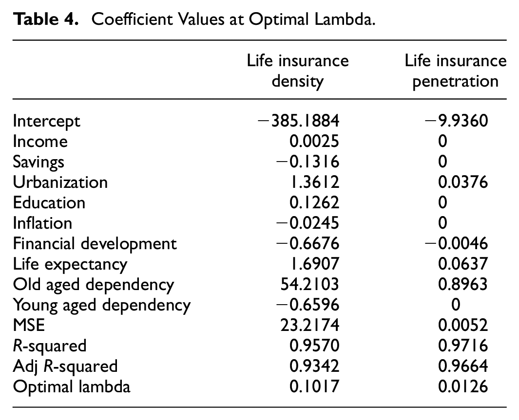
Table 4 shows the values of coefficients corresponding to the optimal lambda (the resulting models). These values have been shrunk and are not the same as the values obtainable from the use of least squared estimations or stepwise regressions. Value of zero means that predictor has been eliminated from the respective model at the optimal lamda. Both the R-squared and the adjusted R-squared are shown for both models. R-squared for models 1 and 2 are 0.9570 and 0.9716 respectively. The adjusted R-squared for models 1 and 2 are 0.9342 and 0.9664 respectively.

Table 4.

Coefficient Values at Optimal Lambda.

	Life insurance density	Life insurance penetration
Intercept	−385.1884	−9.9360
Income	0.0025	0
Savings	−0.1316	0
Urbanization	1.3612	0.0376
Education	0.1262	0
Inflation	−0.0245	0
Financial development	−0.6676	−0.0046
Life expectancy	1.6907	0.0637
Old aged dependency	54.2103	0.8963
Young aged dependency	−0.6596	0
MSE	23.2174	0.0052
R-squared	0.9570	0.9716
Adj R-squared	0.9342	0.9664
Optimal lambda	0.1017	0.0126

Life Insurance Density Determinants (Model 1)

At the optimal lambda of 0.1017, none of the predictors of life insurance density is eliminated from the model. This means that all the predictors are relevant in determining life insurance density as far as the model is concerned. Meanwhile, some predictors have their coefficients more shrunk than the others, based on their relative relevance in the model. The predictor with the largest coefficient is the old aged dependency ratio, followed by life expectancy, urbanization, young dependency ratio, financial development, savings, education, inflation, and finally, income. (It can be seen that the five coefficients with the least values are the very ones reduced to zero in the model 2.)

Savings, inflation, financial development, and young aged dependency have negative relationship with insurance density while old aged dependency, life expectancy, urbanization, education, and income have positive relation with insurance density. Savings having negative relation with life insurance demand is a confirmation that life insurance premium is regarded as a substitute to saving at the bank or investment in financial securities. This means that the more people save in the bank, the less likely they would buy life insurance products. By extension, the more the financial sector develops (particularly the banking sector), the less the demand for life insurance products. Hence financial development also has negative relation with life insurance density. For inflation, it is obviously a threat to investment in financial instruments, particularly those not linked to inflation. Inflation erodes the value of investments, so it has negative relation with life insurance density, per the results. Young aged dependency ratio has negative relationship with life insurance demand. This means that the more young-dependents one has, the less likely it is for the person to buy insurance. This may be due to the financial pressure resulting from payment of school fees and similar expenditures.

Old aged dependency ratio is positively related to life insurance density. This means that people tend to buy more life insurance products when they have old aged dependents on them. Probably, people prefer buying insurance products such as annuity investments and funeral plans for old aged dependents. Life expectancy also has positive relation with life insurance density. This confirms the potential demand for annuity policies by or for the aged. The longer people live, the more they require reliable cash flows in the form of annuity payments. Urbanization has positive relation with life insurance density and this supports the fact that awareness of life insurance and the marketing of same is more vibrant in the urban areas. Again people living in the urban areas are more educated and enlightened, and they know the relevance of life insurance. Per the results, both education and income also have positive relation with life insurance density.

Life Insurance Penetration Determinants (Model 2)

At the optimum lambda of 0.0126, five out of the nine predictors are eliminated from the model. These are income, savings, education, inflation, and young aged dependency ratio. From the correlation matrix, income, education, and young aged dependency ratio have high pairwise correlation with insurance penetration. However, they also appear to have high pairwise correlation with urbanization (a predictor). So the algorithm, through the optimization process, retains urbanization, while income, education, and young dependency ratio are eliminated. The retained predictors of insurance penetration at the optimal lambda are urbanization, financial development, life expectancy, and old aged dependency ratio. Once again, it can be seen that the four retained predictors of insurance penetration are also the four most dominant predictors of insurance density. Furthermore, the retained predictors have the same relationship with insurance penetration, as they do with insurance density. That is, those having positive relation with insurance penetration also have positive relation with insurance density (urbanization, life expectancy, and old aged dependency ratio). Same way, those having negative relation with insurance penetration also have negative relation with insurance density (financial development).

Conclusion, Policy Implication, and Recommendation

The purpose of the study is to model the determinants of life insurance demand, using the elastic net regression algorithm. The elastic net is a hybrid of LASSO regression and ridge regression. Life insurance density and life insurance penetration are used as proxies for life insurance demand. Per the results, it is found that the main macroeconomic and demographic determinants of life insurance demand (both life insurance density and life insurance penetration) are old aged dependency ratio, life expectancy, urbanization, and financial development. The first three have positive relation with life insurance demand while the last one has negative relation with life insurance demand. The fact that old aged dependency ratio has positive relation with life insurance demand is in line with the findings of Redzuan (2014) but somehow contradicts with Akhter and Khan (2017) who argue that larger family size can be a burden on financial resources of primary wage earners, thereby reducing demand for life insurance. However, the negative relation between young dependent ratio and insurance demand is consistent with Akhter and Khan (2017). Life expectancy is positively related to life insurance demand and this supports Sulaiman et al. (2015) who find that life expectancy is positively associated with life insurance. The positive relation between urbanization and life insurance demand supports Zerriaa et al. (2017) who find that high level of urbanization stimulates life insurance demand in Tunisia. The negative relation between financial development and life insurance demand is an emphasis of the fact that the life insurance companies are in competition with the major players in the financial sector—the banks. People choose between saving at the bank, and paying life insurance premium, in anticipation of obtaining a lump sum amount upon maturity. This is in turn consistent with the findings that old dependency ratio and life expectancy have positive relation with life insurance. People prefer using life insurance for investment purposes toward old age, rather than for risk management (or risk transfer). People pay premiums for some number of years, so that they are given some lump sum in the future (at old age) or are paid some series of cash flows when they are on retirement (or at old age). (This is also consistent with the fact that life insurance density is negatively related to savings at the bank, life insurance is considered a substitute of savings.) In addition to investing for future cash flows for the aged while alive, some dependents also buy policies that would cushion them financially in organizing funerals upon the demise of old aged dependents (funeral policies).

The findings of the study have important policy implications. For instance, people see life insurance as being more of investment (or savings) option than as a risk management option. Hence there needs to be a sensitization by government or the regulator (NIC) on the importance of risk management, and the use of life insurance for risk management.

In addition, the following recommendations are made

Since demand for life insurance is largely driven by old aged dependency ratio, and to some extent by life expectancy, more attractive and innovative policies should be made available to entice more aged people to patronize insurance policies.

The younger people should also be encouraged to buy life insurance policies designed to suit their age group.

As urbanization drives life insurance patronage, it means that insurance companies can increase insurance demand if they replicate what happens in the urban areas in the rural or less developed areas. For instance, they can increase insurance demand by increasing their presence in the rural areas through branch outlets and promotions. The closer they get to the people, the more likely the people will patronize the insurance policies.

Often, more enlightened and educated people are found in the urban areas. Education makes the urban dwellers appreciate the relevance of risk management. Therefore, the National Insurance Commission should intensify education aimed at financial literacy, risk management, and insurance, in the rural areas. The more educated the people become, the more likely they will appreciate the need for insurance.

Finally, people should be educated that they can still buy life insurance cover even when they are saving at the bank. Life insurance is largely for risk management purpose, and not only for investment purpose.

Contribution of the Study

Unlike previous studies which used least square estimations and stepwise regressions to determine life insurance demand, this study uses the elastic net algorithm (a regularization algorithm). This algorithms is best suited for modeling under the circumstance of multicollinearity. The algorithm also improves the out-of-sample prediction of the model. Regularized regression methods are more robust than least squares methods. It is worthy of note that this is the first study which seeks to model the macroeconomic and demographic determinants of life insurance using the elastic net algorithm.

Limitation of the Study

The study only covers the period 1994 through 2020. Other years were not covered due to lack of data. Secondly, the study only considers life insurance demand. Non-life insurance demand is not considered by this study.

Suggestion for Further Studies

We recommend this study is extended, to model non-life insurance demand using the elastic net algorithm.

Footnotes

Declaration of Conflicting Interests

The author(s) declared no potential conflicts of interest with respect to the research, authorship, and/or publication of this article.

Funding

The author(s) received no financial support for the research, authorship, and/or publication of this article.

Ethical Approval

The study does not seem to breach any ethical requirement. Data used for the study is secondary data which is a publicly available.

ORCID iDs

Phyllis Asorh Oteng

Victor Curtis Lartey

References

Akhter

Khan

S. U.

(2017). Determinants of Takāful and conventional insurance demand: A regional analysis. Cogent Economics & Finance, 5, 1–18.

Alhassan

A. L.

Biekpe

(2016). Determinants of life insurance consumption in Africa. Research in International Business and Finance, 37, 17–27.

Ampaw

Nketiah-Amponsah

Owoo

N. S.

(2018). Gender perspective on life insurance demand in Ghana. International Journal of Social Economics, 45, 1631–1646.

Anderson

D. R.

Nevin

J. R.

(1975). Determinants of young married’s life insurance purchasing behavior: An empirical investigation. The Journal of Risk and Insurance, 42, 375–387.

Athey

(2017). Beyond prediction: Using big data for policy problems. Science, 355, 483–485.

Auerbach

A. T.

Kotlikoff

L. J.

(1989). How rational is the purchase of life insurance? (NBER Working Paper No. 3063). https://ssrn.com/abstract=227470

Babbel

D. F.

(1981). Inflation, indexation and life insurance sales in Brazil. The Journal of Risk and Insurance, 48, 115–135.

Beck

Webb

(2003). Economic, demographic, and institutional determinants of life insurance consumption across countries. World Bank Economic Review, 17, 51–88.

Browne

Kim

(1993). An international analysis of life insurance demand. The Journal of Risk and Insurance, 60, 616–634.

10.

Buonaccorsi

J. P.

(1996). A modified estimating equation approach to correcting for measurement error in regression. Biometrika, 83, 433–440.

11.

Curak

Dzaja

Pepur

(2013). The effect of social and demographic factors on life insurance demand in Croatia. International Journal of Business and Social Science, 4, 65–72.

12.

Ćurak

Gašpić

K. M.

(2011). Economic and social determinants of life insurance consumption: Evidence from central and eastern Europe. The Journal of American Academy of Business, Cambridge, 16, 216–222.

13.

Dorugade

A. V.

(2014). New ridge parameters for ridge regression. Journal of the Association of Arab Universities for Basic and Applied Sciences, 15, 94–99.

14.

Dragos

S. L.

(2014). Life and non-life insurance demand: The different effects of influence factors in emerging countries from Europe and Asia. Economic Research-Ekonomska Istraživanja, 27, 169–180.

15.

Duker

J. M.

(1969). Expenditures for life insurance among working-wife families. The Journal of Risk and Insurance, 36, 525–533.

16.

Enz

(2000). The S-curve relation between per-capita income and insurance penetration. The Geneva Papers on Risk and Insurance—Issues and Practice, 25, 396–406.

17.

Feyen

Lester

Rocha

(2011). What drives the development of the insurance sector? An empirical analysis based on a panel of developed and developing countries (Working Paper No. 5572). World Bank Policy Research.

18.

Finch

W. H.

Finch

M. E. H.

(2016). Regularization methods for fitting linear models with small sample sizes: Fitting the lasso estimator using R. Practical Assessment, Research & Evaluation, 21, 1531–7714.

19.

Fofie

G. A.

(2016). What influence customer patronage of insurance policies: An empirical assessment of socio-economic and demographic determinants of insurance patronage in Ghana. International Review of Management and Marketing, 6, 81–88.

20.

Ghanaweb. (2019). Insurance industry contribution to GDP not encouraging—Senior Minister. Retrieved May 1, 2019, from https://www.ghanaweb.com/GhanaHomePage/business/Insurance-industry-contribution-to-GDP-not-encouraging-Senior-Minister-733640

21.

Greene

M. R.

(1954). Life insurance buying in inflation. Journal of the American Association of University Teachers of Insurance, 21, 99–113.

22.

Guerineau

Sawadogo

(2015). On the determinants of life insurance development in Sub-Saharan Africa: The role of the institutions quality in the effect of economic development (Working Paper No. halshs-01178838). HAL.

23.

Hammond

J. D.

Houston

D. B.

Melander

E. R.

(1967). Determinants of household life insurance premium expenditures: An empirical investigation. The Journal of Risk and Insurance, 34, 397–408.

24.

Hoerl

Kennard

(1970). Ridge regression: Biased estimation for nonorthogonal problems. Technometrics, 12, 55–67.

25.

Hwang

Gao

(2003). The determinants of the demand for life insurance in an emerging economy: The case of China. Managerial Finance, 29, 82–96.

26.

Iyawe

O. O.

Osamwonyi

I. O.

(2017). Financial development and life insurance demand in sub-Sahara Africa. International Journal of Financial Research, 8, 163–175.

27.

Kalra

Fan

Sinha

(2013). Urbanization in emerging markets: Boon and bane for insurers. SwissRe Sigma. http://media.swissre.com/documents/sigma5_2013_en.pdf

28.

Kleinberg

Ludwig

Mullainathan

Rambachan

(2018). Algorithmic fairness. AEA Papers and Proceedings, 108, 22–27.

29.

Lenten

L. J.

Rulli

D. N.

(2006). A time-series analysis of the demand for life insurance companies in Australia: An unobserved components approach. Australian Journal of Management, 31, 41–66.

30.

Lewis

F. D.

(1989). Dependents and the demand for life insurance. The American Economic Review, 79, 452–467.

31.

Moshirian

Nguyen

Wee

(2007). The demand for life insurance in OECD countries. The Journal of Risk and Insurance, 74, 637–652.

32.

Mapharing

Otuteye

Radikoko

(2015). Determinants of demand for life insurance: The case of Canada. Journal of Comparative International Management, 18, 1–22.

33.

Mullainathan

Spiess

(2017). Machine learning: An applied econometric approach. Journal of Economic Perspectives, 31, 87–106.

34.

National Insurance Commission. (2019). Annual Report.

35.

Nesterova

(2008). Determinants of the demand for life insurance: Evidence from selected CIS and CEE Countries [Masters thesis]. National University “Kyiv-Mohyla Academy”.

36.

Outreville

J. F.

(1996). Life insurance markets in developing countries. The Journal of Risk and Insurance, 63, 263–278.

37.

Park

Lemaire

(2012). The impact of culture on the demand for non-life insurance. ASTIN Bulletin: The Journal of the IAA, 42, 501–527.

38.

Peprah

J. A.

Koomson

Forson

(2017). Demand for insurance in Ghana: Do poverty, employment status and demographic characteristics matter? (NESRA Working Paper No. 17/001). NESRA.

39.

Redzuan

(2014). Analysis of the demand for life insurance and family takāful. Australian Academy of Business and Social Sciences Conference 2014. Retrieved May 1, 2019, from https://www.aabss.org.au/system/files/published/AABSS2014_290.pdf

40.

Schwebler

(1984). Identification and quantification of the overall impact of the national economy on life assurance in the Federal Republic of Germany. The Geneva Papers on Risk and Insurance, 9, 280–298.

41.

Sen

(2008). An analysis of life insurance demand determinants for selected Asian economies and India (Working Paper No. 36/2008). Retrieved May 2, 2019, from http://www.eaber.org/system/tdf/documents/MSE_Sen_2008.pdf?file=1&type=node&id=22512&force=

42.

Sen

Madheswaran

(2007). Are life insurance demand determinants valid for selected Asian economies and India?APRIA 11th Annual Conference—Asia-Pacific Risk and Insurance Association, Taipei, National Chengchi University.

43.

Smith

(2018). Step away from stepwise. Journal of Big Data, 5, 1–12.

44.

Sulaiman

L.A.

Migiro

Yeshihareg

(2015). Investigating the factors influencing the life insurance market in Ethiopia. Problems and Perspectives in Management, 13, 152–160.

45.

The Mathworks. (2021). Regularization (Ridge regression, lasso, elastic nets). https://www.mathworks.com/help/stats/regularization-1.html

46.

Tibshirani

(1996). Regression shrinkage and selection via the lasso. Journal of the Royal Statistical Society: Series B (Methodological), 58, 267–288.

47.

Treerattanapun

(2011). The impact of culture on non-life insurance consumption. Wharton Research Scholars, 78, 1–24.

48.

Truett

D. B.

Truett

L. J.

(1990). The Demand for life insurance in Mexico and the United States: A comparative study. The Demand for Life Insurance in Mexico and the United States: A Comparative Study, 57, 321–328.

49.

Varian

H. R.

(2014). Big data: New tricks for econometrics. Journal of Economic Perspectives, 28, 3–28.

50.

Yuan

Jiang

(2015). Factors affecting the demand for insurance in China. Applied Economics, 47, 4855–4867.

51.

Zerriaa

Amiri

M. M.

Noubbigh

Naoui

(2017). Determinants of life insurance demand in Tunisia. African Development Review, 29, 69–80.

52.

Zhang

Zhu

(2005). Determinants of the development of insurance in China under the globalization. Retrieved May 1, 2019, from https://pdfs.semanticscholar.org/5b03/2f2e73daba3584185301f73be197250e7fe9.pdf?_ga=2.135536433.185787915.1557255366-2045149507.1550245207

53.

Zou

Hastie

(2005). Regularization and variable selection via the elastic net. Journal of the Royal Statistical Society: Series B (Methodological), 67, 301–320.

Modeling the Macroeconomic and Demographic Determinants of Life Insurance Demand in Ghana Using the Elastic Net Algorithm

Abstract

Keywords

Introduction

Multicollinearity and Regularization

Literature Review

Life Insurance Demand

Determinants of Life Insurance Demand

Income

Inflation

Financial Development

Education

Dependency Ratio

Life Expectancy

Savings

Urbanization

Data and Methodology

Dependent Variable

Independent Variables

Income

Savings

Education

Inflation

Financial Development

Dependency Ratio (Old Dependents)

Dependency Ratio (Young Dependents)

Life Expectancy

Urbanization

Model Specification

Mathematical Formulation of the Regularization Problem

Ridge Regression

LASSO Regression

Elastic Net Regression

Results and Discussion

Life Insurance Density Determinants (Model 1)

Life Insurance Penetration Determinants (Model 2)

Conclusion, Policy Implication, and Recommendation

Contribution of the Study

Limitation of the Study

Suggestion for Further Studies

Footnotes

Declaration of Conflicting Interests

Funding

Ethical Approval

ORCID iDs

References