A Best Linear Empirical Bayes Method for High-Dimensional Covariance Matrix Estimation

Abstract

Covariance matrix estimation plays a significant role in both in the theory and practice of portfolio analysis and risk management. This paper deals with the available data prior to developing a factor model to enhance covariance matrix estimation. Our work has two main outcomes. First, for a general linear model with unknown prior parameters, a class of best linear empirical Bayes estimators is established through two kinds of architectures to improve the estimation accuracy by utilizing additional data prior. The theoretical results indicate two key points: the proposed estimators are equivalent to the linear minimum mean-square error estimator when complete or sufficient partial data prior are provided; and the proposed estimators perform better than the optimal weighted least squares method, which ignores the data prior in each situation. Second, the proposed estimators are used for calculating a high-dimensional covariance matrix through factor models. The numerical example and the simulation results verify the effectiveness of our methods.

Introduction

Estimation is a problem concerning how to make the best of the information contained in data for the purpose of inferring an unknown quantity. This information includes the prior information and the observable sample data. The two most popular philosophies for estimation are:

• Classical: the parameter is viewed as an unknown constant (not random) and thus it does not have a (prior, posterior, or marginal) distribution.

• Bayesian: the parameter is regarded as a random variable with a known prior distribution.

The debate between the two schools has been on-going for many decades. Some of the major criticisms leveled are (Robbins, 1983):

• The classical philosophy ignores the existence of any prior information, which makes the inference rely entirely on the sample observation data. This could represent a significant waste of information.

• The Bayesian philosophy forces people to select a prior distribution subjectively and/or arbitrarily and thus the correctness/appropriateness of the inference results is questionable.

The empirical Bayes methodology is a compromise between these two approaches. It assumes that the parameter is a random variable but with an unknown distribution which can be estimated from sample data. In economics, management, and many other disciplines, it is usually difficult for us to obtain any prior knowledge about the parameter, so we usually adopt a classical estimation theory to estimate the parameter, such as the least squares (LS) method. Although it is difficult to obtain prior knowledge of a parameter, we can generally estimate relatively reliable prior knowledge about the data from the sample observation data. Therefore, the empirical Bayes method can be used to deal with this kind of problem. Table 1 contrasts the classical, Bayesian, and empirical Bayes philosophies.

Table 1.

Comparison of Different Estimation Philosophies.

	Classical	Bayesian	Empirical Bayes
Parameter	Unknown constant	Random variable
Parameter prior distribution	Does not exist	Known	Exist but unknown
Sample data prior distribution	Known	Known	Known (could be estimated from sample data)
Likelihood (model)	Known	Known
Posterior distribution	Does not exist	Known

This paper is motivated by the work of X. R. Li et al. (2003) which established and improved the weighted least squares (WLS) estimation, the best linear unbiased estimation (BLUE), and their generalized versions with complete, partial, or no prior knowledge of the parameter. In this work, we consider the widely used linear data model with unknown prior knowledge of the parameter and develop a class of best linear empirical Bayesian (BLEB) estimation methods when the data prior is assumed to be complete or incomplete, identified by two kinds of estimation architectures in explicit forms. The proposed method is essentially a type of Bayesian method that can improve the estimation performance since prior information regarding the data is considered, while this information is ignored in the classical estimation theory.

Covariance matrix estimation plays a significant role both in the theory and practice of portfolio analysis and risk management (De Jong, 2018; Ismail & Pham, 2019; Ledoit & Wolf, 2022; Menchero & Ji, 2021; Wang et al., 2021; Xin & Zhao, 2022). The famous mean-variance portfolio optimization theory of Markowitz (1952) indicates that we can create an optimal portfolio if the expected returns, the variance and the covariance of every asset can be estimated accurately. Therefore, we need an effective and accurate covariance matrix estimation method (Clifford & Feng, 2018; Lan et al., 2018; Wang & Xia, 2021). The importance of covariance matrix estimation has led to the emergence of a large number of estimation methods for covariance matrices in the existing literature (Agrawal et al., 2022; Dong & Tse, 2020; Fan & Mincheva, 2011; Harris & Yilmaz, 2010; Jiang et al., 2023; Ledoit & Wolf, 2003; Stein, 1977; Sun & Xu, 2022; Vassallo et al., 2021). However, high-dimensional covariance matrix estimation is challenging in nature and has been widely studied in recent years (Moura et al., 2020; So et al., 2022; Zhu et al., 2021). Moreover, dimensionality disaster is the main problem in high-dimensional covariance matrix estimation. For instance, in optimal portfolio allocation and portfolio risk assessment, the number of stocks, $p$ , is usually of the same order as the sample size, $n$ , which is in the order of hundreds or thousands. In particular, when $p=200$ , there are more than 10,000 unknown parameters in the covariance matrix to be inferred. However, we may only have roughly $n=260$ by using weekly data for the past five years. Therefore, in this case, it is almost impossible to forecast the covariance matrix accurately without using any structure (Fan, 2005).

Multi-factor models have been commonly used theoretically and empirically in economics, finance and management. The well-known arbitrage pricing theory (APT) proposed by Ross (1976, 1977) shows that the excessive return of assets has a certain relationship with specific factors through a special linear model. In this context, multi-factor models have been widely used and studied, (Aguilar & West, 2000; Alfelt et al., 2022; Bai, 2003; Chamberlain, 1983; Engle & Watson, 1981; Fan et al., 2008). Thanks to these multi-factor models, if several factors can capture the cross-sectional risks completely, the number of parameters to be estimated in the covariance matrix can be reduced significantly (De Nard et al., 2021; X. L. Li et al., 2022). For instance, taking a three-factor model as an example, there are only $4p$ instead of $p(p+1)/2$ unknown parameters (Fan et al., 2008).

Moreover, when estimating a high-dimensional covariance matrix with a multi-factor model, the most critical aspect is the estimation of factor loadings or factor returns. When all or part of the prior information for the parameter is known, we can use the linear minimum mean-square error (LMMSE) estimation proposed by X. R. Li et al. (2003) to obtain the optimal linear unbiased estimator for the parameter, while prior information for factor loadings or factor returns is rarely impossible to obtain, and thus the classical LS estimator is commonly used for estimation. However, although it is difficult for us to obtain prior information for the parameter, prior information for asset returns can usually be summarized roughly from historical data or experience, so an estimation method that does not consider any prior information wastes a lot of prior information contained in sample data.

Generally speaking, the more abundant the prior information is, the higher the estimation accuracy will be. Therefore, in order to make full use of the available information, we first use the BLEB estimator proposed in this paper to estimate the factor loadings or factor returns, and then calculate the high-dimensional covariance matrix through the factor models.

Linear Estimation With a Linear Data Model

Linear estimation is extremely popular mainly due to its simplicity. There have been many theoretical achievements in linear estimation. Invented by Gauss in 1795, the LS approach is the oldest and one of the simplest methods for classical estimation philosophies. The WLS method treats the parameter as an unknown constant and makes inferences relying only on the sample observation data. Another famous linear estimation method, developed and perfected by X. R. Li et al. (2003), is the LMMSE estimator. LMMSE is a Bayesian method that views the parameter as a random variable and performs the estimation by combining the prior information for the parameter and the current sample observation data. These two well-known estimators are simple but powerful. Next, we will briefly introduce the linear data model, the WLS estimator, and the LMMSE estimator, which will be used and compared in the next Section.

Linear Data Model

Consider the linear data model:

$$y_i=X_i\mathrm{\beta }+{\epsilon }_i,i=1,2,3,...,n$$

(1)

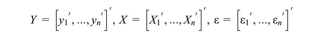
where vector $y_i$ is the sample data, $X_i$ is a matrix that is not a function of parameters vector $\mathrm{\beta }$ and ${\epsilon }_i$ is the error, or more compactly

$$Y=X\mathrm{\beta }+\epsilon$$

(2)

with

$$Y={[{y_1}^{\prime },...,{y_n}^{\prime }]}^{\prime },X={[{X_1}^{\prime },...,{X_n}^{\prime }]}^{\prime },\epsilon ={[{{\epsilon }_1}^{\prime },...,{{\epsilon }_n}^{\prime }]}^{\prime }$$

The error $\epsilon$ has a mean $\overline{\epsilon }$ and its covariance matrix is given as $R=\mathrm{cov}\left(\epsilon \right)$ . In general, $R$ is given as a nonsingular diagonal matrix and $X$ is a full column rank matrix.

Weighted Least-Squares Estimator (Classical Philosophy)

The linear WLS estimator of an unknown but nonrandom vector $\mathrm{\beta }$ using sample data $Y$ is the estimator that minimizes the quadratic fitting error:

$$J={(Y-X\hat{\mathrm{\beta }})}^{\prime }W(Y-X\hat{\mathrm{\beta }})$$

where the weighting matrix $W>O$ is symmetric.

Minimizing $J$ gives the linear WLS estimator:

$${\hat{\mathrm{\beta }}}^{\mathrm{WLS}}={(X\prime \mathrm{WX})}^{-1}X\prime W(Y-\overline{\epsilon })$$

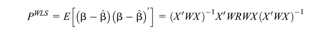
with the estimation error covariance matrix:

$$P^{\mathrm{WLS}}=E\left[(\mathrm{\beta }-\hat{\mathrm{\beta }}){(\mathrm{\beta }-\hat{\mathrm{\beta }})}^{\prime }\right]={(X\prime \mathrm{WX})}^{-1}X\prime \mathrm{WRWX}{(X\prime \mathrm{WX})}^{-1}$$

$P^{\mathrm{WLS}}$ is minimized by choosing the optimal weighting matrix $W=R^{-1}$ , and:

$$P^{\mathrm{OWLS}}=P_{min}^{\mathrm{WLS}}=\underset{W}{min}{P}^{\mathrm{WLS}}={(X\prime R^{-1}X)}^{-1}$$

where the optimal WLS estimator (OWLS) is:

$${\hat{\mathrm{\beta }}}^{\mathrm{OWLS}}={(X\prime R^{-1}X)}^{-1}X\prime R^{-1}(Y-\overline{\epsilon })$$

(3)

It can be seen that the linear WLS estimator is always unbiased and the OWLS estimator in fact minimizes the error covariance matrix of all linear unbiased estimators using linear data model (2) for a non-random parameter. In particular, when we choose the weighted matrix $W=I$ , we can obtain the classical LS estimator

$$\begin{array}{c}{\hat{\mathrm{\beta }}}^{\mathrm{LS}}={(X\prime X)}^{-1}X\prime (Y-\overline{\epsilon })\hfill \\ P^{\mathrm{LS}}={(X\prime X)}^{-1}X\prime \mathrm{RX}{(X\prime X)}^{-1}\hfill \end{array}$$

(4)

Linear Minimum Mean-Square Error Estimator (LMMSE; Bayesian Philosophy)

The LMMSE estimator is a linear Bayesian estimator of a random vector $\mathrm{\beta }$ with additional prior information:

$$\overline{\mathrm{\beta }}=E\left(\mathrm{\beta }\right),C_{\mathrm{\beta }}=\mathrm{cov}\left(\mathrm{\beta }\right),C_{\mathrm{\beta }\epsilon }=\mathrm{cov}(\mathrm{\beta },\epsilon )$$

Under the linear data model (2), we have:

$$\begin{array}{c}\overline{Y}=X\overline{\mathrm{\beta }}+\overline{\epsilon }\hfill \\ C_{\mathrm{\beta }Y}=C_{\mathrm{\beta }}X\prime +C_{\mathrm{\beta }\epsilon }\hfill \\ C_Y=X{C}_{\mathrm{\beta }}X\prime +R+X{C}_{\mathrm{\beta }\epsilon }+{\left(X{C}_{\mathrm{\beta }\epsilon }\right)}^{\prime }\hfill \end{array}$$

It can be seen that the error $\epsilon$ and the parameter $\mathrm{\beta }$ are usually uncorrelated (i.e., $C_{\mathrm{\beta }\epsilon }=O$ ) in many practical problem; thus:

$$C_Y=X{C}_{\mathrm{\beta }}X\prime +R$$

The LMMSE estimator is the one that is linear (actually affine) in the data $Y$ and minimizes the following mean-square error (MSE) matrix:

$$P=E\left[(\mathrm{\beta }-\hat{\mathrm{\beta }}){(\mathrm{\beta }-\hat{\mathrm{\beta }})}^{\prime }\right]$$

Minimizing $P$ gives the LMMSE estimator:

$$\begin{array}{c}{\hat{\mathrm{\beta }}}^{\mathrm{LMMSE}}=\arg \underset{\hat{\mathrm{\beta }}=\mathrm{AY}+b}{min}P=\overline{\mathrm{\beta }}+C_{\mathrm{\beta }Y}{C}_Y^{-1}(Y-\overline{Y})\hfill \\ P^{\mathrm{LMMSE}}=C_{\mathrm{\beta }}-C_{\mathrm{\beta }Y}{C}_Y^{-1}{C\prime }_{\mathrm{\beta }Y}\hfill \end{array}$$

(5)

The above results are valid if $C_Y^{-1}$ is replaced with the Moore–Penrose inverse $C_Y^{+}$ when the inverse of $C_Y$ is singular.

The above LMMSE estimator is unbiased and is the best linear estimator for $\mathrm{\beta }$ with known prior information (and thus a BLUE).

It can be seen that the OWLS estimator ${\mathrm{\beta }}^{\mathrm{OWLS}}$ in Section 2.2 is also called a BLUE, with the assumption that $\mathrm{\beta }$ is a non-random constant vector without the concept of prior information. When we view the parameter $\mathrm{\beta }$ as a random vector with known prior information, the BLUE of the linear data model (2) is the LMMSE estimator ${\hat{\mathrm{\beta }}}^{\mathrm{LMMSE}}$ .

As previously stated, in many research fields, such as the multi-factor model, we are seriously short of direct prior knowledge of the parameter, so LMMSE estimation with complete prior information cannot be directly used. Considering that the prior of the sample data is important for the final estimation accuracy, we will study the specific form of the linear empirical Bayes estimator under the general linear data model (2) in Section 3.

Best Linear Empirical Bayes Estimators (BLEB) With a Linear Data Model

Assumptions

For linear estimation, prior knowledge, in general, refers only to the knowledge of the first two moments of random vectors $\{\overline{\mathrm{\beta }},\overline{Y},\overline{\epsilon },C_{\mathrm{\beta }},C_Y,R,C_{\mathrm{\beta }\epsilon ,}{C}_{\mathrm{\beta }Y}\}$ as mentioned in Section 2. In the Bayesian framework, all of these eight moments are existing and known. In the classical non-Bayesian philosophy, however, the parameter $\mathrm{\beta }$ is an unknown constant vector, thus the prior $\{\overline{\mathrm{\beta }},C_{\mathrm{\beta }}\}$ does not exist. Since the error $\epsilon$ is also viewed as a random vector in the classical school, $\{\overline{Y},\overline{\epsilon },C_Y,R,C_{\mathrm{\beta }\epsilon ,}{C}_{\mathrm{\beta }Y}\}$ exists under the linear data model (2) with $\overline{Y}=X\mathrm{\beta }+\overline{\epsilon },C_{\mathrm{\beta }Y}=C_{\mathrm{\beta }\epsilon }=O,C_Y=R$ .

As stated before, the empirical Bayes method holds that $\{\overline{\mathrm{\beta }},C_{\mathrm{\beta }}\}$ exists but is unknown, which can be estimated from the known true data prior $\{\overline{Y},C_Y\}$ or the approximate data prior $\{\hat{\overline{Y}},{\hat{C}}_Y\}$ that can be inferred from the sample observation data.

Now considering the linear data model (2), we define the best linear empirical Bayes (BLEB) estimators as linear (actually affine) in the data $Y$ and minimize the MSE matrix with two different kinds of assumptions:

• A. Complete data prior means all elements in $\overline{Y},C_Y$ , and $C_{\epsilon Y}$ are known;

• B. Partial data prior means some but not all elements in $\overline{Y},C_Y$ , and $C_{\epsilon Y}$ are known.

BLEB Estimators With Complete Data Prior

We develop two architectures to deal with this problem from different perspectives.

Express the Prior for the Parameter Explicitly

For convenience, we say that a BLEB estimator is has complete data prior if both the prior mean and the covariance of the sample data $Y$ (as well as its correlation with the error $\epsilon$ ) are known, because the only prior knowledge of the sample data used by a BLEB estimator is its first two moments. Using the data model (2), the BLEB estimator with complete data prior can always be inferred by the first two moments of $\epsilon$ and $Y$ . In other words, we can express the unknown $\{\overline{\mathrm{\beta }},C_{\mathrm{\beta }}\}$ in terms of the known complete data prior $\{\overline{Y},C_Y,C_{\epsilon Y}\}$ . The following theorem presents the BLEB estimator in the case of complete data prior for data model (2).

• Theorem 1 (BLEB estimator with complete data prior). Using data model (2), the BLEB estimator with complete data prior $\overline{Y}=E\left(Y\right)$ , $C_Y=\mathrm{cov}(Y)$ , and $C_{\epsilon Y}=\mathrm{cov}(\epsilon ,Y)$ is:

$$\begin{array}{c}\hat{\mathrm{\beta }}=X^{+}[Y-\overline{\epsilon }-C_{\epsilon Y}{C}_Y^{+}(Y-\overline{Y})]\hfill \\ P=X^{+}(R-C_{\epsilon Y}{C}_Y^{+}{C_{\epsilon Y}}^{\prime }){\left(X^{+}\right)}^{\prime }\hfill \end{array}$$

(6)

where the superscript + stands for the Moore–Penrose inverse, and for a full column rank matrix $X$ , we have $X^{+}={(X\prime X)}^{-1}X\prime$ . Usually, $\mathrm{\beta }$ and $\epsilon$ are uncorrelated and in this case we have:

$$\begin{array}{c}\hat{\mathrm{\beta }}=X^{+}[Y-\overline{\epsilon }-{\mathrm{RC}}_Y^{+}(Y-\overline{Y})]\hfill \\ P=X^{+}(R-{\mathrm{RC}}_Y^{+}R){\left(X^{+}\right)}^{\prime }\hfill \end{array}$$

(7)

• Proof: See the Appendix.

Remarks:

• Without using the prior for parameter $\mathrm{\beta }$ , the BLEB estimator with complete data prior is equivalent to the LMMSE estimator in (5) and thus a BLUE. It outperforms the OWLS estimator in formula (3) which does not use any prior information. This will be described in detail later in Theorem 5.

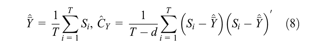
• In practice, $\mathrm{\beta }$ and $\epsilon$ are usually assumed to be uncorrelated. However, the exact data prior $\{\overline{Y},C_Y,C_{\epsilon Y}\}$ are usually unknown but can be estimated by the past sampling data, as in the general empirical Bayes methodology. For instance, given a set of (past) data $\{S_1,...,S_T\}$ and (current) sample data $Y$ , where $S_i$ and $Y$ have the same dimension $d$ , the practical BLEB estimator is obtained by replacing $\{\overline{Y},C_Y\}$ in formula (7) with their sample mean:

$$\hat{\overline{Y}}=\frac{1}{T}\sum _{i=1}^T{S}_i,{\hat{C}}_Y=\frac{1}{T-d}\sum _{i=1}^T(S_i-\hat{\overline{Y}}){(S_i-\hat{\overline{Y}})}^{\prime }$$

(8)

and this converges to the theoretical result in formula (7) under very general conditions due to the famous law of large numbers.

Treat the Prior Mean of the Sample Data as Data

For the linear data model (2), the problem of obtaining the BLEB estimator with complete data prior can always be converted to a problem of obtaining a BLUE estimator without any prior, as given by the Lemma 1 as follows.

• Lemma 1: Given complete data prior $\{\overline{Y},C_Y,C_{\epsilon Y}\}$ , the problem of obtaining a BLEB estimator with complete data prior for the linear data model (2) can always be converted to obtain a BLUE estimator without any known prior. This can be achieved by treating the prior mean of sample data as an extra data using the following augmented linear data model (assume that $\mathrm{\beta }$ and $\epsilon$ are uncorrelated):

$$Y_A=X_A\mathrm{\beta }+{\epsilon }_A$$

(9)

with:

$$\begin{array}{c}\multicolumn{1}{c}{Y_A=\left[\begin{array}{c}\overline{Y}\hfill \\ \multicolumn{1}{c}{Y}\end{array}\right],X_A=\left[\begin{array}{c}X\hfill \\ \multicolumn{1}{c}{X}\end{array}\right],{\overline{\epsilon }}_A=E\left({\epsilon }_A\right)=\left[\begin{array}{c}\overline{Y}-X\mathrm{\beta }\hfill \\ \multicolumn{1}{c}{\epsilon }\end{array}\right]}\\ \multicolumn{1}{c}{=\left[\begin{array}{c}\overline{\epsilon }\hfill \\ \multicolumn{1}{c}{\overline{\epsilon }}\end{array}\right],R_A=\mathrm{cov}\left({\epsilon }_A\right)=\left[\begin{array}{cc}{C}_Y-R\hfill & 0\hfill \\ \multicolumn{1}{c}{0}& R\hfill \end{array}\right]}\end{array}$$

• Proof: See the Appendix.

The following theorem presents a BLUB estimator without any known prior using the data model (9).

• Theorem 2 (BLEB estimator with complete data prior by treating the prior mean of the sample data as data). Using data model (9), the BLEB estimator by treating the prior mean $\overline{Y}$ of sample data $Y$ as data is:

$$\begin{array}{c}\hat{\mathrm{\beta }}=L(Y_A-{\overline{\epsilon }}_A)=K(Y_A-{\overline{\epsilon }}_A)\hfill \\ P=L{R}_{A}L\prime =K{R}_{A}K\prime ={\left({X\prime }_A{R}_A^{+}{X}_A\right)}^{-1}\hfill \\ K={\left({X\prime }_A{R}_A^{+}{X}_A\right)}^{-1}{X\prime }_A{R}_A^{+}\hfill \\ L=K+\mathrm{MN}\hfill \end{array}$$

(10)

where $N=I-X_A{X}_A^{+}$ , $M$ is any matrix satisfying ${\mathrm{MNR}}_A^{1/2}=O$ , and $R_A^{1/2}$ is any square-root matrix of $R_A$ . This estimator is unique almost surely and it is equal to $K(Y_A-{\overline{\epsilon }}_A)$ .

It can be seen that the error covariance matrix $R_A$ in the data model (9) is always singular since $X_A$ is full column rank.

• Proof: See the Appendix.

Remarks:

• This theorem shows that for optimal linear estimation, data prior can always be completely embedded into the linear data model (9) by viewing the prior mean as observation data. The BLEB estimator (10) is algebraically equivalent to the BLEB estimator (7) since they both use the same information just in different ways. The equivalence will be discussed and proved in Theorem 5.

• The above equivalence reveals that the prior information can also be viewed as a kind of observation data, and thus the BLEB estimator (10) can be thought of as a unification of Bayesian and classical linear estimators.

• It is noticed that, the form of the BLEB estimator (10) is similar to the OWLS estimator (3). However, the parameter $\mathrm{\beta }$ is random here which is different from the OWLS estimator, and the optimization objective here is the MSE matrix, not the fitting error in WLS, despite the OWLS also optimizing the MSE with non-random $\mathrm{\beta }$ . Details can be found in the poof of Theorem 2.

• In practice, the estimated ${\hat{R}}_A$ may be nonsingular and then the BLEB estimator (10) will degenerate into

$$\hat{\mathrm{\beta }}={\left(X_A{\hat{R}}_A^{-1}{X}_A\right)}^{-1}{X}_A{\hat{R}}_A^{-1}(Y_A-{\overline{\epsilon }}_A),P={\left(X_A{\hat{R}}_A^{-1}{X}_A\right)}^{-1}$$

BLEB Estimators With Partial Data Prior

Similar to Section 3.2, we consider using two architectures to deal with this problem from different perspectives.

Express the Prior for the Parameter Explicitly

In reality, sometimes the corresponding moments $\{\overline{Y},C_Y,C_{\epsilon Y}\}$ do not fully exist. This would be the case where some but not all components of data prior $\overline{Y},C_Y$ , and $C_{\epsilon Y}$ are available. For instance, there can be some newly listed assets when we estimate the mean and covariance of the return of assets from historical sample observation data. In this case, it is almost impossible to estimate relatively accurate prior for these newly listed assets from a few sample data. Therefore, we generally think that there is no data prior for these newly listed assets.

Let $Z=[Z_1,Z_2]=\mathrm{QY}$ , where $Q=[Q_1,Q_2]$ is an orthogonal matrix $Q^{-1}=Q\prime$ , and $Z_1=Q_{1}Y$ is the subvector of $Z$ that corresponds to a nonsingular $\mathrm{\Lambda }$ in the sense that $C_{Z_1}=\mathrm{cov}\left(Z_1\right)=\mathrm{\Lambda }$ . Then the partial data prior can be denoted as $\{{\overline{Z}}_1,C_{Z_1},C_{\epsilon Z_1}\}$ .

Using data model (2), the BLEB estimator with partial data prior can sometimes be inferred by the first two moments of $\epsilon$ and $Y$ . In other words, we can express the unknown $\{\overline{\mathrm{\beta }},C_{\mathrm{\beta }}\}$ in terms of the known sufficient partial data prior of $\{\overline{Y},C_Y,C_{\epsilon Y}\}$ . Theorem 3 gives the BLEB estimator with sufficient partial data prior. It can be seen that, in this paper, sufficient partial data prior means that $Q_{1}X$ is full column rank and insufficient partial data prior means that $Q_{1}X$ is not full column rank.

• Theorem 3 (BLEB estimator with sufficient partial data prior). Given $Q_{1}X$ of full column rank, and uncorrelated $\mathrm{\beta }$ and $\epsilon$ , by using data model (2), the BLEB estimator with sufficient partial data prior $\{{\overline{Z}}_1,\mathrm{\Lambda }\}$ is:

$$\begin{array}{c}\hat{\mathrm{\beta }}=\overline{\mathrm{\beta }}+C_{\mathrm{\beta }Y}{C}_Y^{+}(Y-\overline{Y})\hfill \\ P=C_{\mathrm{\beta }}-C_{\mathrm{\beta }Y}{C}_Y^{+}{C\prime }_{\mathrm{\beta }Y}\hfill \end{array}$$

(11)

where the superscript + stands for MP inverse, and:

$$\begin{array}{c}\multicolumn{1}{c}{\overline{\mathrm{\beta }}={\left(Q_{1}X\right)}^{+}[{\overline{Z}}_1-Q_1\overline{\epsilon }]}\\ \multicolumn{1}{c}{\overline{Y}=X{\left(Q_{1}X\right)}^{+}[{\overline{Z}}_1-Q_1\overline{\epsilon }]+\overline{\epsilon }}\\ \multicolumn{1}{c}{C_{\mathrm{\beta }}={\left(Q_{1}X\right)}^{+}(\mathrm{\Lambda }-Q_{1}R{Q_1}^{\prime }){{\left(Q_{1}X\right)}^{+}}^{\prime }}\\ \multicolumn{1}{c}{C_{\mathrm{\beta }Y}={\left(Q_{1}X\right)}^{+}(\mathrm{\Lambda }-Q_{1}R{Q_1}^{\prime }){{\left(Q_{1}X\right)}^{+}}^{\prime }X\prime }\\ \multicolumn{1}{c}{C_Y=X{\left(Q_{1}X\right)}^{+}(\mathrm{\Lambda }-Q_{1}R{Q_1}^{\prime }){{\left(Q_{1}X\right)}^{+}}^{\prime }X\prime +R}\end{array}$$

• Proof: See the Appendix.

Remarks:

• Without using the prior for parameter $\mathrm{\beta }$ explicitly, the BLEB estimator with sufficient partial data prior (i.e., $Q_{1}X$ is full column rank) is equivalent to the LMMSE estimator in (5) and thus a BLUE. It outperforms the OWLS estimator in (3) which does not use any prior information. This will be described in detail later in Theorem 5.

• is full column rank, which is a necessary condition in this theorem for expressing the prior for the parameter explicitly and uniquely.

Treat the Prior Mean of the Sample Data as Data

Similar to Theorem 2, for the linear model (2), the problem of obtaining a BLEB estimator with partial data prior can also be converted to a problem of obtaining a BLUE estimator without any prior, as presented in Lemma 2 as follows.

• Lemma 2: Given partial data prior $\{{\overline{Z}}_1,\mathrm{\Lambda }\}$ , the problem of obtaining a BLEB estimator with partial data prior for the linear data model (2) can always be converted to obtain a BLUE estimator without known prior by treating the partial prior mean of the sample data as extra data using the following augmented linear data model (assume that $\mathrm{\beta }$ and $\epsilon$ are uncorrelated):

$$Y_A=X_A\mathrm{\beta }+{\epsilon }_A$$

(12)

with

$$\begin{array}{c}\multicolumn{1}{c}{Y_A=\left[\begin{array}{c}{\overline{Z}}_1\hfill \\ \multicolumn{1}{c}{Y}\end{array}\right],{\overline{\epsilon }}_A=E\left({\epsilon }_A\right)=\left[\begin{array}{c}{Q}_1\overline{\epsilon }\hfill \\ \multicolumn{1}{c}{\overline{\epsilon }}\end{array}\right],X_A=\left[\begin{array}{c}{Q}_{1}X\hfill \\ \multicolumn{1}{c}{X}\end{array}\right],}\\ \multicolumn{1}{c}{R_A=\mathrm{cov}\left({\epsilon }_A\right)=\left[\begin{array}{cc}\mathrm{\Lambda }-Q_{1}R{Q\prime }_1\hfill & 0\hfill \\ \multicolumn{1}{c}{0}& R\hfill \end{array}\right]}\end{array}$$

• Proof: See the Appendix.

Similarly, once ${\overline{Z}}_1$ is treated as sample observation data, there is no data information about $Y$ at all. Further, obviously, the form of the data model (12) is the same as that of the data model (9). The BLEB estimator with partial data prior is then given in the following Theorem 4.

• Theorem 4 (BLEB estimator with partial data prior by treating the prior mean of the sample data as data). Given partial data prior $\{{\overline{Z}}_1,\mathrm{\Lambda }\}$ and using data model (12), the BLEB estimator with partial data prior has the same form as that of the BLEB estimator (10) in Theorem 2:

$$\begin{array}{c}\hat{\mathrm{\beta }}=L(Y_A-{\overline{\epsilon }}_A)=K(Y_A-{\overline{\epsilon }}_A)\hfill \\ P=L{R}_{A}L\prime =K{R}_{A}K\prime ={\left({X\prime }_A{R}_A^{+}{X}_A\right)}^{-1}\hfill \\ K={\left({X\prime }_A{R}_A^{+}{X}_A\right)}^{-1}{X\prime }_A{R}_A^{+}\hfill \\ L=K+\mathrm{MN}\hfill \end{array}$$

(13)

except with

$$\begin{array}{c}\multicolumn{1}{c}{Y_A=\left[\begin{array}{c}{\overline{Z}}_1\hfill \\ \multicolumn{1}{c}{Y}\end{array}\right],{\overline{\epsilon }}_A=E\left({\epsilon }_A\right)=\left[\begin{array}{c}{Q}_1\overline{\epsilon }\hfill \\ \multicolumn{1}{c}{\overline{\epsilon }}\end{array}\right],X_A=\left[\begin{array}{c}{Q}_{1}X\hfill \\ \multicolumn{1}{c}{X}\end{array}\right],}\\ \multicolumn{1}{c}{R_A=\mathrm{cov}\left({\epsilon }_A\right)=\left[\begin{array}{cc}\mathrm{\Lambda }-Q_{1}R{Q\prime }_1\hfill & 0\hfill \\ \multicolumn{1}{c}{0}& R\hfill \end{array}\right]}\end{array}$$

and the other matrices are defined in the same way as in the BLEB estimator (10).

Note that the error covariance $R_A$ here is singular, and it depends on whether $Q_{1}X$ in the data model (12) is full column rank or not.

• Proof: See the Appendix.

Remarks:

• The BLEB estimator proposed in Theorem 3 is also a BLUE with the corresponding assumption.

• The BLEB estimator in Theorem 3 is essentially equivalent to the BLEB estimator with complete data prior in Theorem 1 and 2 when sufficient partial data prior is given. This makes sense as the prior knowledge of data $Y$ or $Z_1$ is actually redundant in this situation. Then the complete prior for parameter $\mathrm{\beta }$ can be totally expressed by the complete data prior in $Y$ or $Z_1$ . In other words, the sufficient partial data prior $\{{\overline{Z}}_1,\mathrm{\Lambda },C_{\epsilon Z_1}\}$ is the same as the complete data prior $\{\overline{Y},C_Y,C_{\epsilon Y}\}$ with respect to the complete prior for $\mathrm{\beta }$ , since $Q_{1}X$ is full column rank. This will be stated and proved in detail in Theorem 4.

• What is more serious is that when insufficient partial data prior is given (i.e., $Q_{1}X$ is not full column rank). In this case, the loss of partial data prior information will lead to a worse BLEB estimator which will have a larger MSE matrix than the BLEB estimator using sufficient partial or complete data prior. However, the BLEB estimator with insufficient partial data prior still has a smaller MSE matrix than the OWLS estimator since more information has been used. This will also be stated and proved in detail in Theorem 5.

• In practice, the estimated data prior is not equal to its theoretical value, and thus the final estimated results with partial data prior are different from the one which uses complete data prior even if sufficient partial data prior is given. Generally speaking, no matter whether $Q_{1}X$ is full column rank or not, the practical BLEB estimator using complete estimated data prior $\{\hat{\overline{Y}},{\hat{C}}_Y,{\hat{C}}_{\epsilon Y}\}$ will perform better than that using partial estimated data prior $\{{\hat{\overline{Z}}}_1,\hat{\mathrm{\Lambda }},{\hat{C}}_{\epsilon Z_1}\}$ , since $\{\hat{\overline{Y}},{\hat{C}}_Y,{\hat{C}}_{\epsilon Y}\}$ usually contains more data information than $\{{\hat{\overline{Z}}}_1,\hat{\mathrm{\Lambda }},{\hat{C}}_{\epsilon Z_1}\}$ in most practical situations.

Equivalence and Relationships

The remarks of the previous theorem have mentioned the equivalence of the BLEB estimators (7), (10), (11), and (13) with a full column rank matrix $Q_{1}X$ . The remarks have also stated some important relationships among these different linear estimators under different assumptions. The following Theorem 5 will present the concrete quantitative relationships among several classical, Bayesian, and empirical Bayes linear estimators that have been mentioned or proposed in this article.

• Theorem 5 (relationships). Assume that $\{\overline{\mathrm{\beta }},\overline{Y},\overline{\epsilon },C_{\mathrm{\beta }},C_Y,R,C_{\mathrm{\beta }\epsilon ,}{C}_{\mathrm{\beta }Y}\}$ are all existing while different BLUE estimators can only use corresponding known prior information since they have their own prior assumptions, as previously stated. Then the LS estimator, the OWLS estimator, the LMMSE estimator, and the BLEB estimators proposed in Theorems 1, 2, 3, and 4 exist and must have the following relationships:

$${\hat{\mathrm{\beta }}}^{\mathrm{BLEB}-C}\iff {\hat{\mathrm{\beta }}}^{\mathrm{BLEB}-\mathrm{CT}}\iff {\hat{\mathrm{\beta }}}^{\mathrm{BLEB}-S}\iff {\hat{\mathrm{\beta }}}^{\mathrm{BLEB}-\mathrm{ST}}\iff {\hat{\mathrm{\beta }}}^{\mathrm{LMMSE}}$$

(14)

$${\hat{\mathrm{\beta }}}^{\mathrm{BLEB}-C}\stackrel{\mathrm{beat}}{\to }{\hat{\mathrm{\beta }}}^{\mathrm{BLEB}-\mathrm{IST}}\stackrel{\mathrm{beat}}{\to }{\hat{\mathrm{\beta }}}^{\mathrm{OWLS}}\stackrel{\mathrm{beat}}{\to }{\hat{\mathrm{\beta }}}^{\mathrm{LS}}$$

(15)

and their MSE matrices have the relationships:

$$\begin{array}{c}\multicolumn{1}{c}{P^{\mathrm{BLEB}-C}=P^{\mathrm{BLEB}-\mathrm{CT}}=P^{\mathrm{BLEB}-S}=P^{\mathrm{BLEB}-\mathrm{ST}}=P^{\mathrm{LMMSE}}}\\ \multicolumn{1}{c}{P^{\mathrm{BLEB}-C}=P^{\mathrm{BLEB}-\mathrm{CT}}={[X\prime {(C_Y-R)}^{+}X+X\prime R^{-1}X]}^{-1}}\\ \multicolumn{1}{c}{P^{\mathrm{BLEB}-S}=P^{\mathrm{BLEB}-\mathrm{ST}}}\\ \multicolumn{1}{c}{={[X\prime {Q\prime }_1{(\mathrm{\Lambda }-Q_{1}R{Q\prime }_1)}^{+}{Q}_{1}X+X\prime R^{-1}X]}^{-1}}\\ \multicolumn{1}{c}{(Q_{1}X\mathrm{is}\mathrm{full}\mathrm{column}\mathrm{rank})}\\ \multicolumn{1}{c}{P^{\mathrm{LMMSE}}={[C_{\mathrm{\beta }}^{-1}+X\prime R^{-1}X]}^{-1}}\end{array}$$

$$\begin{array}{c}\multicolumn{1}{c}{P^{\mathrm{BLEB}-C}<P^{\mathrm{BLEB}-\mathrm{IST}}<P^{\mathrm{OWLS}}<P^{\mathrm{LS}}}\\ \multicolumn{1}{c}{P^{\mathrm{BLEB}-\mathrm{IST}}={[X\prime {Q\prime }_1{(\mathrm{\Lambda }-Q_{1}R{Q\prime }_1)}^{+}{Q}_{1}X+X\prime R^{-1}X]}^{-1}}\\ \multicolumn{1}{c}{(Q_{1}X\mathrm{is}\mathrm{not}\mathrm{full}\mathrm{column}\mathrm{rank})}\\ \multicolumn{1}{c}{P^{\mathrm{OWLS}}={(X\prime R^{-1}X)}^{-1}}\\ \multicolumn{1}{c}{P^{\mathrm{LS}}=X^{+}R{X^{+}}^{\prime }}\end{array}$$

Where ${\hat{\mathrm{\beta }}}^{\mathrm{BLEB}-C}$ stands for the BLEB estimator with complete data prior in formula (7), ${\hat{\mathrm{\beta }}}^{\mathrm{BLEB}-\mathrm{CT}}$ stands for the BLEB estimator with complete data prior by treating the prior mean of the sample data as data in formula (10), ${\hat{\mathrm{\beta }}}^{\mathrm{BLEB}-S}$ stands for the BLEB estimator with sufficient partial data prior in formula (11), ${\hat{\mathrm{\beta }}}^{\mathrm{BLEB}-\mathrm{ST}}$ stands for the BLEB estimator with sufficient partial data prior by treating the prior mean of sample data as a data in formula (13), ${\hat{\mathrm{\beta }}}^{\mathrm{BLEB}-\mathrm{IST}}$ stands for the BLEB estimator with insufficient partial data prior by treating the prior mean of the sample data as a data in formula (13), ${\hat{\mathrm{\beta }}}^{\mathrm{LMMSE}}$ stands for the LMMSE estimator in (5), ${\hat{\mathrm{\beta }}}^{\mathrm{OWLS}}$ stands for the OWLS estimator in formula (3), and ${\hat{\mathrm{\beta }}}^{\mathrm{LS}}$ stands for the LS estimator in formula (4).

$P^{\mathrm{BLEB}-C}$ , $P^{\mathrm{BLEB}-\mathrm{CT}}$ , $P^{\mathrm{BLEB}-S}$ , $P^{\mathrm{BLEB}-\mathrm{ST}}$ , $P^{\mathrm{BLEB}-\mathrm{IST}}$ , $P^{\mathrm{LMMSE}}$ , $P^{\mathrm{OWLS}}$ and $P^{\mathrm{LS}}$ represent the MSE matrix of the corresponding estimator with the same superscript, respectively. In addition, “ $\mathrm{\iff }$ ” indicates that the estimation accuracy of the former is the same as that of the latter, while “ $\mathrm{beat}$ ” indicates that the estimation accuracy of the former is higher than that of the latter.

• Proof: See the Appendix.

Remarks:

• The LS estimator ${\hat{\mathrm{\beta }}}^{\mathrm{LS}}$ and the OWLS estimator ${\hat{\mathrm{\beta }}}^{\mathrm{OWLS}}$ mentioned above are both classical linear estimation methods that consider the parameter $\mathrm{\beta }$ as an unknown constant vector for which prior information no longer exists. The LMMSE estimator ${\hat{\mathrm{\beta }}}^{\mathrm{LMMSE}}$ is a Bayesian method that views the parameter as a random vector with known complete prior about $\mathrm{\beta }$ . The other five different BLEB estimators are all empirical Bayes estimation methods that also treat the parameter as a random vector but with unknown prior information.

• As stated before, all these estimators presented in Theorem 5 are BLUEs with their corresponding special assumptions, except for the LS estimator ${\hat{\mathrm{\beta }}}^{\mathrm{LS}}$ . The LS estimator will become a BLUE when the error covariance matrix $R={\sigma }^{2}I$ is given.

• Theorem 5 shows that the more prior information is used, the more accurate the estimation result will be. This makes good sense: we should try to make the most of the prior information even if it can only be estimated from sample observation data.

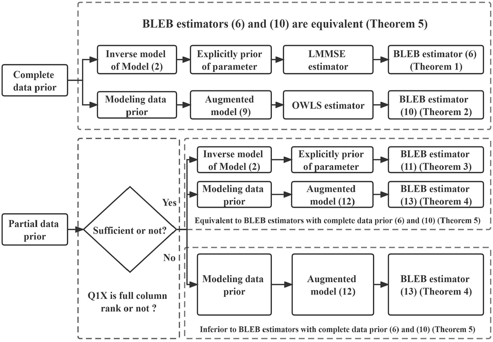
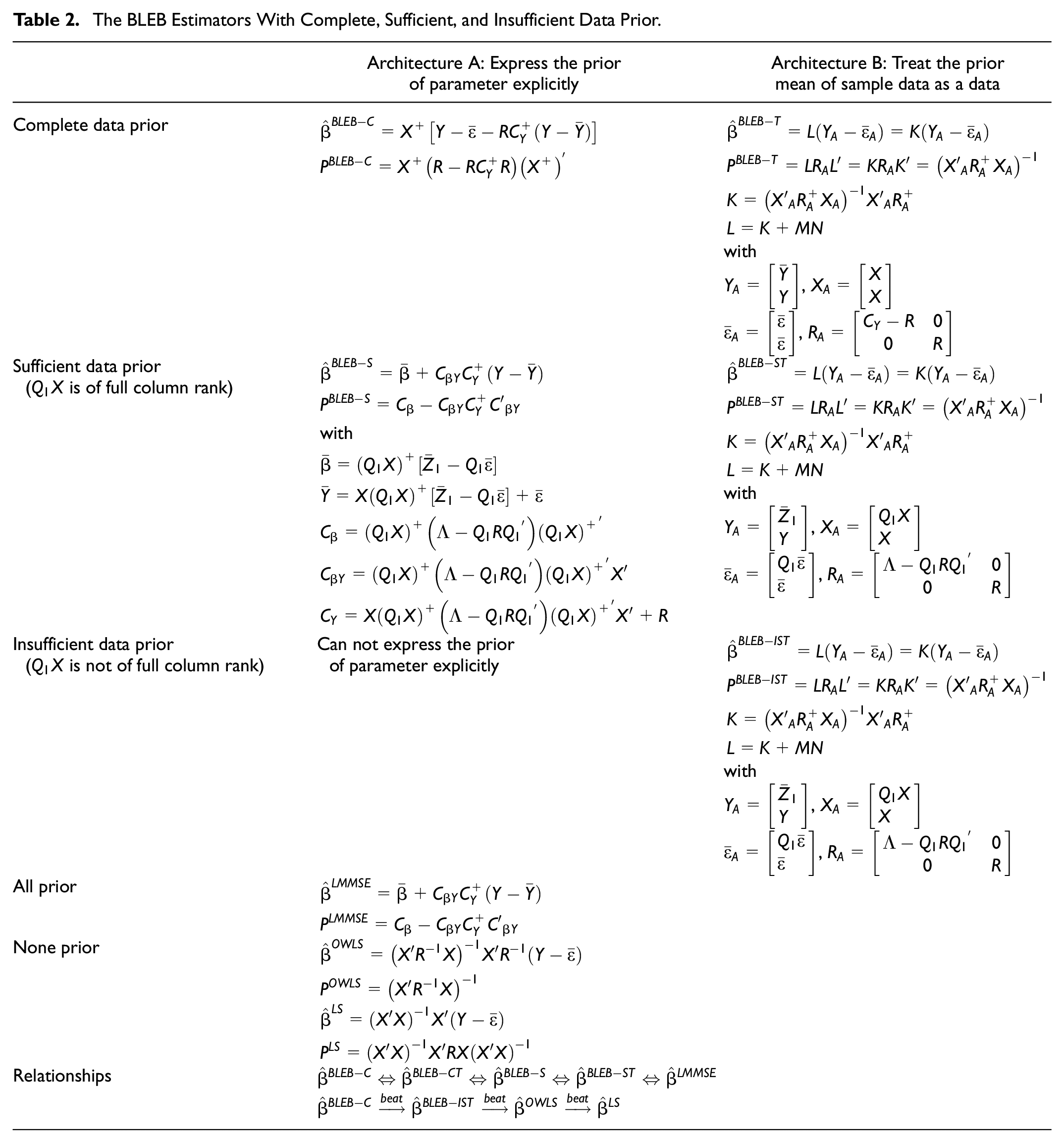
In order to make the use of Theorems 1 to 5 clearer, the flow chart of the BLEB methods with different assumptions of data prior is shown in Figure 1. In addition, Table 2 summarizes the BLEB estimators and the other BLUE estimators for ease of employment.

Figure 1.

Flow chart of the BLEB methods with different assumptions of data prior.

Table 2.

The BLEB Estimators With Complete, Sufficient, and Insufficient Data Prior.

	Architecture A: Express the prior of parameter explicitly	Architecture B: Treat the prior mean of sample data as a data
Complete data prior	$\begin{array}{c}\multicolumn{1}{c}{{\hat{\mathrm{\beta }}}^{\mathrm{BLEB}-C}=X^{+}[Y-\overline{\epsilon }-{\mathrm{RC}}_Y^{+}(Y-\overline{Y})]}\\ \multicolumn{1}{c}{P^{\mathrm{BLEB}-C}=X^{+}(R-{\mathrm{RC}}_Y^{+}R){\left(X^{+}\right)}^{\prime }}\end{array}$	$\begin{array}{c}\multicolumn{1}{c}{{\hat{\mathrm{\beta }}}^{\mathrm{BLEB}-T}=L(Y_A-{\overline{\epsilon }}_A)=K(Y_A-{\overline{\epsilon }}_A)}\\ \multicolumn{1}{c}{P^{\mathrm{BLEB}-T}=L{R}_{A}L\prime =K{R}_{A}K\prime ={\left({X\prime }_A{R}_A^{+}{X}_A\right)}^{-1}}\\ \multicolumn{1}{c}{K={\left({X\prime }_A{R}_A^{+}{X}_A\right)}^{-1}{X\prime }_A{R}_A^{+}}\\ \multicolumn{1}{c}{L=K+\mathrm{MN}}\end{array}$ with $Y_A=\left[\begin{array}{c}\overline{Y}\hfill \\ \multicolumn{1}{c}{Y}\end{array}\right]$ , $X_A=\left[\begin{array}{c}X\hfill \\ \multicolumn{1}{c}{X}\end{array}\right]$ ${\overline{\epsilon }}_A=\left[\begin{array}{c}\overline{\epsilon }\hfill \\ \multicolumn{1}{c}{\overline{\epsilon }}\end{array}\right]$ , $R_A=\left[\begin{array}{c}{C}_Y-R0\hfill \\ \multicolumn{1}{c}{0R}\end{array}\right]$
Sufficient data prior ( $Q_{1}X$ is of full column rank)	$\begin{array}{c}\multicolumn{1}{c}{{\hat{\mathrm{\beta }}}^{\mathrm{BLEB}-S}=\overline{\mathrm{\beta }}+C_{\mathrm{\beta }Y}{C}_Y^{+}(Y-\overline{Y})}\\ \multicolumn{1}{c}{P^{\mathrm{BLEB}-S}=C_{\mathrm{\beta }}-C_{\mathrm{\beta }Y}{C}_Y^{+}{C\prime }_{\mathrm{\beta }Y}}\\ \multicolumn{1}{c}{\mathrm{with}}\\ \multicolumn{1}{c}{\overline{\mathrm{\beta }}={\left(Q_{1}X\right)}^{+}[{\overline{Z}}_1-Q_1\overline{\epsilon }]}\\ \multicolumn{1}{c}{\overline{Y}=X{\left(Q_{1}X\right)}^{+}[{\overline{Z}}_1-Q_1\overline{\epsilon }]+\overline{\epsilon }}\\ \multicolumn{1}{c}{C_{\mathrm{\beta }}={\left(Q_{1}X\right)}^{+}(\mathrm{\Lambda }-Q_{1}R{Q_1}^{\prime }){{\left(Q_{1}X\right)}^{+}}^{\prime }}\\ \multicolumn{1}{c}{C_{\mathrm{\beta }Y}={\left(Q_{1}X\right)}^{+}(\mathrm{\Lambda }-Q_{1}R{Q_1}^{\prime }){{\left(Q_{1}X\right)}^{+}}^{\prime }X\prime }\\ \multicolumn{1}{c}{C_Y=X{\left(Q_{1}X\right)}^{+}(\mathrm{\Lambda }-Q_{1}R{Q_1}^{\prime }){{\left(Q_{1}X\right)}^{+}}^{\prime }X\prime +R}\end{array}$	$\begin{array}{c}\multicolumn{1}{c}{{\hat{\mathrm{\beta }}}^{\mathrm{BLEB}-\mathrm{ST}}=L(Y_A-{\overline{\epsilon }}_A)=K(Y_A-{\overline{\epsilon }}_A)}\\ \multicolumn{1}{c}{P^{\mathrm{BLEB}-\mathrm{ST}}=L{R}_{A}L\prime =K{R}_{A}K\prime ={\left({X\prime }_A{R}_A^{+}{X}_A\right)}^{-1}}\\ \multicolumn{1}{c}{K={\left({X\prime }_A{R}_A^{+}{X}_A\right)}^{-1}{X\prime }_A{R}_A^{+}}\\ \multicolumn{1}{c}{L=K+\mathrm{MN}}\end{array}$ with $Y_A=\left[\begin{array}{c}{\overline{Z}}_1\hfill \\ \multicolumn{1}{c}{Y}\end{array}\right]$ , $X_A=\left[\begin{array}{c}{Q}_{1}X\hfill \\ \multicolumn{1}{c}{X}\end{array}\right]$ ${\overline{\epsilon }}_A=\left[\begin{array}{c}{Q}_1\overline{\epsilon }\hfill \\ \multicolumn{1}{c}{\overline{\epsilon }}\end{array}\right]$ , $R_A=\left[\begin{array}{c}\mathrm{\Lambda }-Q_{1}R{Q_1}^{\prime }0\hfill \\ \multicolumn{1}{c}{0R}\end{array}\right]$
Insufficient data prior ( $Q_{1}X$ is not of full column rank)	Can not express the prior of parameter explicitly	$\begin{array}{c}\multicolumn{1}{c}{{\hat{\mathrm{\beta }}}^{\mathrm{BLEB}-\mathrm{IST}}=L(Y_A-{\overline{\epsilon }}_A)=K(Y_A-{\overline{\epsilon }}_A)}\\ \multicolumn{1}{c}{P^{\mathrm{BLEB}-\mathrm{IST}}=L{R}_{A}L\prime =K{R}_{A}K\prime ={\left({X\prime }_A{R}_A^{+}{X}_A\right)}^{-1}}\\ \multicolumn{1}{c}{K={\left({X\prime }_A{R}_A^{+}{X}_A\right)}^{-1}{X\prime }_A{R}_A^{+}}\\ \multicolumn{1}{c}{L=K+\mathrm{MN}}\end{array}$ with $Y_A=\left[\begin{array}{c}{\overline{Z}}_1\hfill \\ \multicolumn{1}{c}{Y}\end{array}\right]$ , $X_A=\left[\begin{array}{c}{Q}_{1}X\hfill \\ \multicolumn{1}{c}{X}\end{array}\right]$ ${\overline{\epsilon }}_A=\left[\begin{array}{c}{Q}_1\overline{\epsilon }\hfill \\ \multicolumn{1}{c}{\overline{\epsilon }}\end{array}\right]$ , $R_A=\left[\begin{array}{c}\mathrm{\Lambda }-Q_{1}R{Q_1}^{\prime }0\hfill \\ \multicolumn{1}{c}{0R}\end{array}\right]$
All prior	$\begin{array}{c}\multicolumn{1}{c}{{\hat{\mathrm{\beta }}}^{\mathrm{LMMSE}}=\overline{\mathrm{\beta }}+C_{\mathrm{\beta }Y}{C}_Y^{+}(Y-\overline{Y})}\\ \multicolumn{1}{c}{P^{\mathrm{LMMSE}}=C_{\mathrm{\beta }}-C_{\mathrm{\beta }Y}{C}_Y^{+}{C\prime }_{\mathrm{\beta }Y}}\end{array}$
None prior	$\begin{array}{c}\multicolumn{1}{c}{{\hat{\mathrm{\beta }}}^{\mathrm{OWLS}}={(X\prime R^{-1}X)}^{-1}X\prime R^{-1}(Y-\overline{\epsilon })}\\ \multicolumn{1}{c}{P^{\mathrm{OWLS}}={(X\prime R^{-1}X)}^{-1}}\end{array}$ $\begin{array}{c}\multicolumn{1}{c}{{\hat{\mathrm{\beta }}}^{\mathrm{LS}}={(X\prime X)}^{-1}X\prime (Y-\overline{\epsilon })}\\ \multicolumn{1}{c}{P^{\mathrm{LS}}={(X\prime X)}^{-1}X\prime \mathrm{RX}{(X\prime X)}^{-1}}\end{array}$
Relationships	${\hat{\mathrm{\beta }}}^{\mathrm{BLEB}-C}\iff {\hat{\mathrm{\beta }}}^{\mathrm{BLEB}-\mathrm{CT}}\iff {\hat{\mathrm{\beta }}}^{\mathrm{BLEB}-S}\iff {\hat{\mathrm{\beta }}}^{\mathrm{BLEB}-\mathrm{ST}}\iff {\hat{\mathrm{\beta }}}^{\mathrm{LMMSE}}$ ${\hat{\mathrm{\beta }}}^{\mathrm{BLEB}-C}\stackrel{\mathrm{beat}}{\to }{\hat{\mathrm{\beta }}}^{\mathrm{BLEB}-\mathrm{IST}}\stackrel{\mathrm{beat}}{\to }{\hat{\mathrm{\beta }}}^{\mathrm{OWLS}}\stackrel{\mathrm{beat}}{\to }{\hat{\mathrm{\beta }}}^{\mathrm{LS}}$

A Numerical Example

Consider the following linear data model

$$Y_i=X_i\mathrm{\beta }+{\epsilon }_i,X_i=[1,i],i=1,2,3$$

where parameter $\mathrm{\beta }=[{\mathrm{\beta }}_1,{\mathrm{\beta }}_2]\prime$ is a two-dimensional unknown vector to be estimated, $Y=[Y_1,Y_2,Y_3]\prime$ is a random sample, and $[Y_1,Y_2,Y_3]\prime =[2.1,3.2,4.3]\prime$ is a current sample observation data. $\mathrm{\beta }$ and ${\epsilon }_i$ are mutually uncorrelated, $E\left({\epsilon }_i\right)=0$ , $\mathrm{var}\left({\epsilon }_i\right)=i$ , and the prior of parameter and sample data are assumed as:

$$\begin{array}{c}\multicolumn{1}{c}{\overline{\mathrm{\beta }}=\left[\begin{array}{c}1\hfill \\ \multicolumn{1}{c}{1}\end{array}\right],C_{\mathrm{\beta }}=\left[\begin{array}{cc}2\hfill & 1\hfill \\ \multicolumn{1}{c}{1}& 2\hfill \end{array}\right]\mathrm{and}\overline{Y}=\left[\begin{array}{c}2\hfill \\ \multicolumn{1}{c}{3}\\ \multicolumn{1}{c}{4}\end{array}\right],}\\ \multicolumn{1}{c}{C_Y=\left[\begin{array}{ccc}7\hfill & 9\hfill & 12\hfill \\ \multicolumn{1}{c}{9}& 16\hfill & 19\hfill \\ \multicolumn{1}{c}{12}& 19\hfill & 29\hfill \end{array}\right]}\end{array}$$

respectively, and they satisfy the relationship $\overline{Y}=X\overline{\mathrm{\beta }},C_Y=X{C}_{\mathrm{\beta }}X\prime +R$ , where, we denote $X={[{X\prime }_1,{X\prime }_2,{X\prime }_3]}^{\prime }$ , $\epsilon ={[{\epsilon }_1,{\epsilon }_2,{\epsilon }_3]}^{\prime }$ , and $R=\mathrm{cov}\left(\epsilon \right)$ .

• A. The LS estimator assumes that the parameter $\mathrm{\beta }$ is an unknown constant vector, which refuses to accept the existence of the prior information for the parameter presented above. Thus, by using formula (4), we have:

$${\hat{\mathrm{\beta }}}^{\mathrm{LS}}=[1,1.1]\prime ,P^{\mathrm{LS}}\approx \left[\begin{array}{cc}3.33\hfill & -1.67\hfill \\ \multicolumn{1}{c}{-1.67}& 1\hfill \end{array}\right]$$

• B. The OWLS estimator has the same assumption as the LS estimator, and by using formula (3), we have:

$${\hat{\mathrm{\beta }}}^{\mathrm{OWLS}}=[1,1.1]\prime ,P^{\mathrm{OWLS}}\approx \left[\begin{array}{cc}3.00\hfill & -1.50\hfill \\ \multicolumn{1}{c}{-1.50}& 0.92\hfill \end{array}\right]$$

• C. The LMMSE estimator assumes that the complete prior information about $\mathrm{\beta }$ exist and is known as given above; thus by using the formula (5), we have:

$${\hat{\mathrm{\beta }}}^{\mathrm{LMMSE}}\approx [1.04,1.07]\prime ,P^{\mathrm{LMMSE}}\approx \left[\begin{array}{cc}0.70\hfill & -0.30\hfill \\ \multicolumn{1}{c}{-0.30}& 0.26\hfill \end{array}\right]$$

• D. The BLEB estimator with complete data prior assumes the prior of parameter $\mathrm{\beta }$ is unknown but data prior is completely known as given above, then by using the formula (7), we have:

$${\hat{\mathrm{\beta }}}^{\mathrm{BLEB}-C}\approx [1.04,1.07]\prime ,P^{\mathrm{BLEB}-C}\approx \left[\begin{array}{cc}0.70\hfill & -0.30\hfill \\ \multicolumn{1}{c}{-0.30}& 0.26\hfill \end{array}\right]$$

• E. The BLEB estimator with complete data prior by treating the prior mean of the sample data as data has the same assumption as the BLEB estimator with complete data prior, and by using the formula (10), we have:

$${\hat{\mathrm{\beta }}}^{\mathrm{BLEB}-\mathrm{CT}}\approx [1.04,1.07]\prime ,P^{\mathrm{BLEB}-\mathrm{CT}}\approx \left[\begin{array}{cc}0.70\hfill & -0.30\hfill \\ \multicolumn{1}{c}{-0.30}& 0.26\hfill \end{array}\right]$$

• F. The BLEB estimator with sufficient partial prior ( $Q_{1}X)=\left[\begin{array}{ccc}1\hfill & 0\hfill & 0\hfill \\ \multicolumn{1}{c}{0}& 1\hfill & 0\hfill \end{array}\right]\left[\begin{array}{cc}1\hfill & 1\hfill \\ \multicolumn{1}{c}{1}& 2\hfill \\ \multicolumn{1}{c}{1}& 3\hfill \end{array}\right]=\left[\begin{array}{cc}1\hfill & 1\hfill \\ \multicolumn{1}{c}{1}& 2\hfill \end{array}\right]$ is full column rank) assumes that the partial data prior is known as:

$${\overline{Z}}_1=\left[\begin{array}{c}{\overline{Y}}_1\hfill \\ \multicolumn{1}{c}{{\overline{Y}}_2}\end{array}\right]=\left[\begin{array}{c}2\hfill \\ \multicolumn{1}{c}{3}\end{array}\right],\mathrm{\Lambda }=\mathrm{cov}\left({\overline{Z}}_1\right)=\left[\begin{array}{cc}7\hfill & 9\hfill \\ \multicolumn{1}{c}{9}& 16\hfill \end{array}\right]$$

Then, by using the formula (11), we have:

$${\hat{\mathrm{\beta }}}^{\mathrm{BLEB}-S}\approx [1.04,1.07]\prime ,P^{\mathrm{BLEB}-S}\approx \left[\begin{array}{cc}0.70\hfill & -0.30\hfill \\ \multicolumn{1}{c}{-0.30}& 0.26\hfill \end{array}\right]$$

• G. The BLEB estimator with sufficient partial data prior by treating the prior mean of sample data as a data ( $Q_{1}X)=\left[\begin{array}{ccc}1\hfill & 0\hfill & 0\hfill \\ \multicolumn{1}{c}{0}& 1\hfill & 0\hfill \end{array}\right]\left[\begin{array}{cc}1\hfill & 1\hfill \\ \multicolumn{1}{c}{1}& 2\hfill \\ \multicolumn{1}{c}{1}& 3\hfill \end{array}\right]=\left[\begin{array}{cc}1\hfill & 1\hfill \\ \multicolumn{1}{c}{1}& 2\hfill \end{array}\right]$ is of full column rank) assumes that the sufficient partial data prior is known as:

$${\overline{Z}}_1=\left[\begin{array}{c}{\overline{Y}}_1\hfill \\ \multicolumn{1}{c}{{\overline{Y}}_2}\end{array}\right]=\left[\begin{array}{c}2\hfill \\ \multicolumn{1}{c}{3}\end{array}\right],\mathrm{\Lambda }=\mathrm{cov}\left({\overline{Z}}_1\right)=\left[\begin{array}{cc}7\hfill & 9\hfill \\ \multicolumn{1}{c}{9}& 16\hfill \end{array}\right]$$

Then by using the formula (13), we have:

$${\hat{\mathrm{\beta }}}^{\mathrm{BLEB}-\mathrm{ST}}\approx [1.04,1.07]\prime ,P^{\mathrm{BLEB}-\mathrm{ST}}\approx \left[\begin{array}{cc}0.70\hfill & -0.30\hfill \\ \multicolumn{1}{c}{-0.30}& 0.26\hfill \end{array}\right]$$

• H. The BLEB estimator with insufficient partial data prior by treating the prior mean of sample data as a data ( $Q_{1}X)=\left[\begin{array}{ccc}1\hfill & 0\hfill & 0\hfill \end{array}\right]\left[\begin{array}{cc}1\hfill & 1\hfill \\ \multicolumn{1}{c}{1}& 2\hfill \\ \multicolumn{1}{c}{1}& 3\hfill \end{array}\right]=\left[\begin{array}{cc}1\hfill & 1\hfill \end{array}\right]$ is not of full column rank) assumes that the insufficient partial data prior is known as:

$${\overline{Z}}_1={\overline{Y}}_1=2,\mathrm{\Lambda }=\mathrm{cov}\left({\overline{Z}}_1\right)=7$$

Then, by using the formula (13), we have:

$${\hat{\mathrm{\beta }}}^{\mathrm{BLEB}-\mathrm{IST}}\approx [0.98,1.11]\prime ,P^{\mathrm{BLEB}-\mathrm{IST}}\approx \left[\begin{array}{cc}2.67\hfill & -1.37\hfill \\ \multicolumn{1}{c}{-1.37}& 0.86\hfill \end{array}\right]$$

It is easy to check that the estimates and MSEs of $\mathrm{\beta }$ in A-H totally satisfy Theorem 5: the estimates and corresponding MSEs in cases D-G are the same as those in case C, which shows that the BLEB estimators ${\hat{\mathrm{\beta }}}^{\mathrm{BLEB}-C}$ , ${\hat{\mathrm{\beta }}}^{\mathrm{BLEB}-\mathrm{CT}}$ , ${\hat{\mathrm{\beta }}}^{\mathrm{BLEB}-S}$ , and ${\hat{\mathrm{\beta }}}^{\mathrm{BLEB}-\mathrm{ST}}$ are equivalent to the LMMSE estimator ${\hat{\mathrm{\beta }}}^{\mathrm{LMMSE}}$ . The MSE in case H is smaller than that in case B, which shows that the BLEB estimator ${\hat{\mathrm{\beta }}}^{\mathrm{BLEB}-\mathrm{IST}}$ performs better than the classical OWLS estimator ${\hat{\mathrm{\beta }}}^{\mathrm{OWLS}}$ . The MSE in case H is large than those in case E to G, which shows that the BLEB estimator with insufficient data prior ${\hat{\mathrm{\beta }}}^{\mathrm{BLEB}-\mathrm{IST}}$ performs worse than the BLEB estimators with complete or sufficient data prior.

Covariance Matrix Estimation Using the BLEB Estimators

In the case of a large number of assets, it is extremely difficult to forecast the covariance matrix directly and accurately, and the rough estimation of the high-dimensional covariance matrix will be seriously disadvantageous to the optimal allocation of subsequent portfolios. Fan et al. (2008) proposed using multi-factor models to transform the estimation of the high-dimensional asset return covariance matrix into the estimation of the low-dimensional factor covariance matrix (the number of factors is generally much smaller than the number of assets). The following is a detailed description of how to use the BLEB estimators proposed in this paper to forecast the high-dimensional asset return covariance matrix on the basis of the multi-factor model.

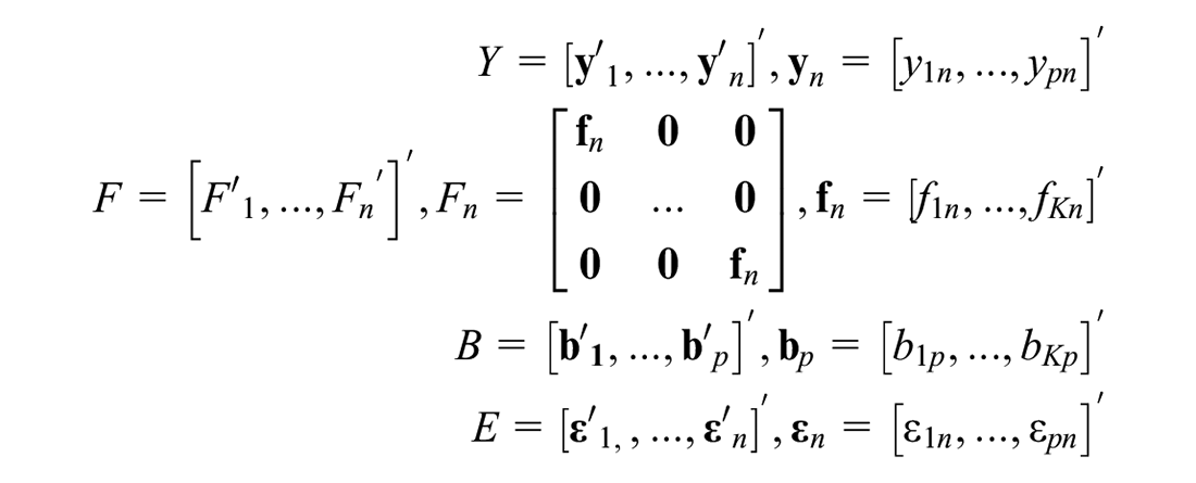
The multi-factor model shows that the excessive returns of assets over the risk-free interest rate satisfies:

$$y_{\mathrm{ij}}=b_{1\mathrm{ij}}{f}_{1\mathrm{ij}}+...+b_{\mathrm{Kij}}{f}_{\mathrm{Kij}}+{\epsilon }_{\mathrm{ij}},i=1,...,p,j=1,...,n$$

(16)

where $p$ and $n$ represent the number of assets and the number of sample return data available for each asset. $f_{1\mathrm{ij}},...,f_{\mathrm{Kij}}$ denotes the factor returns of $K$ factors in the $j$ th sample of asset $i$ . $b_{1\mathrm{ij}},...,b_{\mathrm{Kij}}$ denotes the factor loadings of $K$ factors in the $j$ th sample of asset $i$ , and ${\epsilon }_{\mathrm{ij}}$ is an error term that is unrelated both to factor loadings and factor returns.

Multi-factor models assume a certain relationship among specific factors. These factors can be macroeconomic (unexpected inflation, interest rate changes), fundamental (profit growth, return on net assets, market share), or market-related (beta, industry ownership). There are two common structured models, depending on the type of factors used in the model.

Structured Model 1: Estimating Factor Loadings Given Factor Returns

When using a factor model to forecast the covariance matrix of high-dimensional returns on assets, we first need to estimate factor loadings or factor returns. When the selected factors are macro factors, time series data should be used, that is, multiple sample data ( $n>1$ ). The Fama-French three-factor model is a typical example of these structured models. In this case, factor returns $f_{1\mathrm{ij}},...,f_{\mathrm{Kij}}$ are observable (i.e., known) and are the same for different assets $i$ , while factor loadings $b_{1\mathrm{ij}},...,b_{\mathrm{Kij}}$ are unknown estimated quantities and are the same for different samples $j$ . Then by using the multi-factor model (16), we can obtain get the following specific linear data model:

$$Y=\mathrm{FB}+E$$

(17)

where

$$\begin{array}{c}\multicolumn{1}{c}{Y={[{\mathbf{y}\mathbf{\prime }}_1,...,{\mathbf{y}\mathbf{\prime }}_n]}^{\prime },{\mathbf{y}}_n={[y_{1n},...,y_{\mathrm{pn}}]}^{\prime }}\\ \multicolumn{1}{c}{F={[{F\prime }_1,...,{F_n}^{\prime }]}^{\prime },F_n=\left[\begin{array}{ccc}{\mathbf{f}}_n\hfill & 0\hfill & 0\hfill \\ \multicolumn{1}{c}{0}& ...\hfill & 0\hfill \\ \multicolumn{1}{c}{0}& 0\hfill & {\mathbf{f}}_n\hfill \end{array}\right],{\mathbf{f}}_n={[f_{1n},...,f_{\mathrm{Kn}}]}^{\prime }}\\ \multicolumn{1}{c}{B={[{\mathbf{b}\mathbf{\prime }}_1,...,{\mathbf{b}\mathbf{\prime }}_p]}^{\prime },{\mathbf{b}}_p={[b_{1p},...,b_{\mathrm{Kp}}]}^{\prime }}\\ \multicolumn{1}{c}{E={[{\mathbf{\epsilon }\mathbf{\prime }}_{1\mathbf{,}},...,{\mathbf{\epsilon }\mathbf{\prime }}_n]}^{\prime },{\mathbf{\epsilon }}_n={[{\epsilon }_{1n},...,{\epsilon }_{\mathrm{pn}}]}^{\prime }}\end{array}$$

In addition, under the assumption of independent and identically distributed samples, the first two moments of the augmented sample data $Y$ and the augmented noise $E$ are as follows:

$$\begin{array}{c}\overline{Y}=[\mathbf{\mu },...,\mathbf{\mu }],C_Y=\left[\begin{array}{ccc}\mathrm{\Sigma }\hfill & \mathbf{0}\hfill & \mathbf{0}\hfill \\ \multicolumn{1}{c}{\mathbf{0}}& ...\hfill & \mathbf{0}\hfill \\ \multicolumn{1}{c}{\mathbf{0}}& \mathbf{0}\hfill & \mathrm{\Sigma }\hfill \end{array}\right]\hfill \\ \overline{E}=[\overline{\mathbf{\epsilon }},...,\overline{\mathbf{\epsilon }}],C_E=\left[\begin{array}{ccc}R\hfill & \mathbf{0}\hfill & \mathbf{0}\hfill \\ \multicolumn{1}{c}{\mathbf{0}}& ...\hfill & \mathbf{0}\hfill \\ \multicolumn{1}{c}{\mathbf{0}}& \mathbf{0}\hfill & R\hfill \end{array}\right]\hfill \end{array}$$

where $\mathbf{\mu }$ is the mean of the $p$ -dimensional asset return vector; $\mathrm{\Sigma }$ is the covariance matrix of the $p$ -dimensional asset return vector; and $\overline{\epsilon },R$ are the mean and covariance matrix of the independent and identically distributed error term ${\mathbf{\epsilon }}_{1\mathbf{,}},...,{\mathbf{\epsilon }}_n$ , respectively.

In linear data model (17) using multiple independent samples, the estimated quantity $B$ is a vector consisting of factor loadings, and $F$ is a matrix consisting of observable factor returns. Generally, it is difficult to know the prior information for factor loadings, so the OWLS method (3) without considering the prior data is simply used to estimate $B$ in most of the existing literature. In this paper, from the perspective of making full use of information, the estimators $\{{\hat{\mathbf{\mu }}}_0,{\hat{\mathrm{\Sigma }}}_0\}$ of the mean and covariance matrices using historical sample data or existing experience structures are substituted for the first two moments $\{\mathbf{\mu },\mathrm{\Sigma }\}$ of the return vector of assets and we have

$$\hat{\overline{Y}}=[{\hat{\mathbf{\mu }}}_{\mathbf{0}},...,{\hat{\mathbf{\mu }}}_{\mathbf{0}}],{\hat{C}}_Y=\left[\begin{array}{ccc}{\hat{\mathrm{\Sigma }}}_{\mathbf{0}}\hfill & \mathbf{0}\hfill & \mathbf{0}\hfill \\ \multicolumn{1}{c}{\mathbf{0}}& ...\hfill & \mathbf{0}\hfill \\ \multicolumn{1}{c}{\mathbf{0}}& \mathbf{0}\hfill & {\hat{\mathrm{\Sigma }}}_{\mathbf{0}}\hfill \end{array}\right]$$

In addition, the mean and covariance matrices of errors are unknown in practice and need to be estimated by residual error. We note that the estimate of $\{\overline{\epsilon },R\}$ is $\{\hat{\overline{\epsilon }},\hat{R}\}$ . Now, treating the estimated prior above as the known prior for the sample data in the model (17), and then using the proposed BLEB estimators, we can then obtain a more accurate estimate ${\hat{B}}^{\mathrm{BLEB}}$ of the factor loadings vector $B$ , which is better than the LS estimator commonly used in the existing literature.

After obtaining the estimator of the factor loadings vector ${\hat{B}}^{\mathrm{BELB}}={[{\hat{\mathbf{b}}\mathbf{\prime }}_1,...,{\hat{\mathbf{b}}\mathbf{\prime }}_p]}^{\prime }$ , we can use the following formula to obtain the updated estimator of the covariance matrix $\mathrm{\Sigma }$ for the return on high-dimensional assets:

$$\hat{\mathrm{\Sigma }}={\hat{B}}_m^{\mathrm{BLEB}}{\hat{C}}_f{\hat{B}}_m^{\mathrm{BLEB}\prime }+\hat{R}$$

(18)

where ${\hat{B}}_m^{\mathrm{BLEB}}={[{\hat{\mathbf{b}}}_1,...,{\hat{\mathbf{b}}}_p]}^{\prime }$ is the matrix representation of the estimated factor loadings ${\hat{B}}^{\mathrm{BELB}}$ , and ${\hat{C}}_f$ is the estimator of the observable factor return covariance matrix.

It can be seen that when some elements of prior $\{{\hat{\mathbf{\mu }}}_0,{\hat{\mathrm{\Sigma }}}_0\}$ are not available, such as the assets that have just been listed in the asset vector, we should extract the sub-vector part with known prior for the original asset vector, and use the BLEB estimators with partial data prior proposed in this paper.

Structured Model 2 : Estimating Factor Returns Given Factor Loadings

When the selected factor is the fundamental factor, cross-sectional data analysis should be used. For each cross-section in the sample, there is only one sample for each asset. On the $j$ th cross-section, factor loadings $b_{1\mathrm{ij}},...,b_{\mathrm{Kij}}$ are directly observable (known), while factor returns $f_{1\mathrm{ij}},...,f_{\mathrm{Kij}}$ are the quantities to be estimated and are the same for different assets $i$ . The Barra risk model is a typical example of these structured models (Briner et al., 2009). In this case, by using multi-factor model (16), we can obtain the following specific linear data model:

$$Y_j=B_j{f}_j+{\epsilon }_j$$

(19)

where

$$\begin{array}{c}\multicolumn{1}{c}{Y_j={[y_{1j},...,y_{\mathrm{pj}}]}^{\prime },f={[f_{1j},...,{f_{\mathrm{kj}}}^{\prime }]}^{\prime },\epsilon ={[{\epsilon }_{1j},...,{\epsilon }_{\mathrm{pj}}]}^{\prime }}\\ \multicolumn{1}{c}{B_j={[{\mathbf{b}}_{1j},...,{\mathbf{b}}_{\mathrm{pj}}]}^{\prime },{\mathbf{b}}_{\mathrm{pj}}={[b_{1\mathrm{pj}},...,b_{\mathrm{Kpj}}]}^{\prime }}\end{array}$$

and $E\left({\epsilon }_j\right)={\overline{\epsilon }}_j,\mathrm{cov}\left({\epsilon }_j\right)=R_j$

In addition, under the assumption of independent and identically distributed samples, the first two moments of the sample data $Y_j$ are as follows.

$${\overline{Y}}_j=\mathbf{\mu },C_{Y_j}=\mathrm{\Sigma }$$

where, $\mathbf{\mu }$ is the mean of the $p$ -dimensional asset return vector, and $\mathrm{\Sigma }$ is the covariance matrix of the $p$ -dimensional asset return vector.

In the linear data model (19), the quantity $f_j$ to be estimated is a vector consisting of factor returns on the cross-section $j$ , and $B_j$ is a matrix consisting of observable factor loadings on the cross-section $j$ . Generally, it is difficult to know the prior information for factor returns, so the OWLS method (3) without considering the prior is simply used to estimate $f_i$ in most of the existing literature. In this paper, from the perspective of making full use of information, the estimators $\{{\hat{\mathbf{\mu }}}_0,{\hat{\mathrm{\Sigma }}}_0\}$ of the mean and covariance matrices using historical sample data or existing experience structures are substituted for the first two moments $\{\mathbf{\mu },\mathrm{\Sigma }\}$ of the return vector of assets and we have

$${\hat{\overline{Y}}}_j={\hat{\mathbf{\mu }}}_0,{\hat{C}}_{Y_j}={\hat{\mathrm{\Sigma }}}_0$$

In addition, the mean and covariance matrices of errors are unknown in practice and need to be estimated by residual error. We note that the estimate of $\{{\overline{\epsilon }}_j,R_j\}$ is $\{\hat{\overline{\epsilon }},\hat{R}\}$ . Now, treating the estimated prior above as the known prior for the sample data in the model (19), and then using the proposed BLEB estimators, we can then obtain a more accurate estimate ${{\hat{f}}_j}^{\mathrm{BLEB}}$ of factor loading vector $f_j$ , which is better than the LS estimator commonly used in the existing literature.

By using the above estimation method on $n$ cross-sections, we can obtain an estimator sequence $\{{{\hat{f}}_1}^{\mathrm{BLEB}},...,{{\hat{f}}_n}^{\mathrm{BLEB}}\}$ of the factor returns vector. Using this estimation sequence, we can obtain the sample estimator ${\hat{C}}_f$ of the factor returns covariance matrix. Then, the updated estimator of the covariance matrix of high dimensional asset returns can be obtained by using the following formula:

$$\hat{\mathrm{\Sigma }}=B{\hat{C}}_{f}B+\hat{R}$$

(20)

Where $B$ is a matrix consisting of observable loadings on a cross-section of interest out of the sample.

Similarly, when some elements of prior $\{{\hat{\mathbf{\mu }}}_0,{\hat{\mathrm{\Sigma }}}_0\}$ are not available, such as assets that have just been listed in the asset vector, we should extract the sub-vector part with known prior for the original asset vector, and use the BLEB estimators with partial data prior proposed in this paper.

In order to make our method clearer, Figure 2 shows the flow chart of the BLEB estimators based high-dimensional covariance matrix estimation method.

Figure 2.

Flow chart of the BLEB estimators based high-dimensional covariance matrix estimation method.

Simulation Results

In this section, we use a simulation study to illustrate our theoretical results and to verify the finite-sample performance of our proposed BLEB estimators. Since our primary concern is to verify the practical improvement of estimation accuracy by using our BLEB estimators through factor models, we compare the performance of the proposed BLEB-based covariance matrix estimators only with that of the LS-based covariance matrix estimator using factor models. To contrast different covariance matrix estimators $\hat{\mathrm{\Sigma }}$ to the truth $\mathrm{\Sigma }$ , we examine the estimation error of $\hat{\mathrm{\Sigma }}$ and $\mathrm{\Sigma }$ using the root mean-square error (RMSE) criteria: $\mathrm{EE}\left(\hat{\mathrm{\Sigma }}\right)=\mathrm{RMSE}(\hat{\mathrm{\Sigma }},\mathrm{\Sigma })=\Vert \hat{\mathrm{\Sigma }}-\mathrm{\Sigma }\Vert$ , where $\Vert \mathrm{•}\Vert$ stands for the Frobenius norm.

For simplicity, we fix $K=3$ in our simulation and consider the three-factor model

$$y_{\mathrm{ij}}=b_{1i}{f}_{1j}+b_{2i}{f}_{2j}+b_{3i}{f}_{3j}+{\epsilon }_{\mathrm{ij}},i=1,...,p,j=1,...,$$

(21)

The Fama-French three-factor model (Fama & French, 1992, 1993) is a practical example of the model (21) and is a kind of Structured Model 1 in Section 4.1. In the Fama-French three-factor model, $y_{\mathrm{ij}}$ is the excess return of the $i$ th stock or portfolio. The first factor $f_{1j}$ is the excess return of the proxy of the market portfolio and the other two factors $f_{2j}$ and $f_{3j}$ are created using six value-weighted portfolios based on book-to-market ratio and size.

We take the parameters used in the study of Fan et al. (2008) as our simulation parameters to make our simulation more realistic. The sample means ${\mu }_{F_i},{\mu }_{B_i}$ and sample covariance matrices ${\mathrm{cov}}_{F_i},{\mathrm{cov}}_{B_i}$ of $F_j={[f_{1j},f_{2j},f_{3j}]}^{\prime }$ , $B_i={[b_{1i},b_{2i},b_{3i}]}^{\prime }$ are obtained from a fit of the Fama-French three-factor model using the three-year daily data for 30 industry portfolios from 1 May, 2002 to 29 Aug, 2005 and given as follows (Fan et al., 2008).

$$\begin{array}{c}\multicolumn{1}{c}{{\mu }_{F_j}={[0.0236,0.0130,0.0207]}^{\prime }}\\ \multicolumn{1}{c}{{\mu }_{B_i}={[0.7828,0.5180,0.4100]}^{\prime }}\\ \multicolumn{1}{c}{{\mathrm{cov}}_{F_j}=\left[\begin{array}{ccc}1.2507\hfill & -0.0350\hfill & -0.2042\hfill \\ \multicolumn{1}{c}{-0.0350}& 0.3156\hfill & -0.0023\hfill \\ \multicolumn{1}{c}{-0.2042}& -0.0023\hfill & 0.1930\hfill \end{array}\right]}\\ \multicolumn{1}{c}{{\mathrm{cov}}_{B_i}=\left[\begin{array}{ccc}0.0291\hfill & 0.0239\hfill & 0.0102\hfill \\ \multicolumn{1}{c}{0.0239}& 0.0540\hfill & -0.0070\hfill \\ \multicolumn{1}{c}{0.0102}& -0.0070\hfill & 0.0869\hfill \end{array}\right]}\end{array}$$

In our simulation, we consider comparing five covariance matrix estimators ${\hat{\mathrm{\Sigma }}}_{\mathrm{BLEB}}^T,{\hat{\mathrm{\Sigma }}}_{\mathrm{BLEB}}^C,{\hat{\mathrm{\Sigma }}}_{\mathrm{BLEB}}^{P_{1/2}},{\hat{\mathrm{\Sigma }}}_{\mathrm{BLEB}}^{P_{1/3}},{\hat{\mathrm{\Sigma }}}_{\mathrm{LS}}$ , and the definition of these five estimators is described in Table 3.

Table 3.

The Covariance Matrix Estimators Compared in Simulations.

Estimator	Explanation
${\hat{\mathrm{\Sigma }}}_{\mathrm{BLEB}}^T$	The BLEB based covariance matrix estimator with true complete data prior
${\hat{\mathrm{\Sigma }}}_{\mathrm{BLEB}}^C$	The BLEB based covariance matrix estimator with estimated complete data prior
${\hat{\mathrm{\Sigma }}}_{\mathrm{BLEB}}^{P_{1/2}}$	The BLEB based covariance matrix estimator with estimated half data prior (only half assets prior are assumed known)
${\hat{\mathrm{\Sigma }}}_{\mathrm{BLEB}}^{P_{1/3}}$	The BLEB based covariance matrix estimator with estimated one third data prior (only one third assets prior are assumed known)
${\hat{\mathrm{\Sigma }}}_{\mathrm{LS}}$	The LS based covariance matrix estimator without using any data prior

Then we take the following steps for each simulation:

• Generate $n$ random samples of $F_j={[f_{1j},f_{2j},f_{3j}]}^{\prime }$ from the trivariate normal distribution $N({\mu }_{F_j},{\mathrm{cov}}_{F_j})$ as the sample data to be used for estimation.

• Generate $p$ factor loadings vectors $B_i={[b_{1i},b_{2i},b_{3i}]}^{\prime }$ as random samples from the trivariate normal distribution $N({\mu }_{B_i},{\mathrm{cov}}_{B_i})$ .

• Generate $p$ standard deviations ${\sigma }_1,...,{\sigma }_p$ from a gamma distribution $G(\alpha ,\mathrm{\beta })$ with $\alpha =3.3586,\mathrm{\beta }=0.1876$ (Fan et al., 2008).

• Generate $n$ random samples $E_j={[{\epsilon }_{1j},...,{\epsilon }_{\mathrm{pj}}]}^{\prime }$ from the $p$ -variate normal distribution $N(0,\mathrm{diag}({\sigma }_1^2,...,{\sigma }_p^2))$ .

• From model (21), we obtain random samples $y_{\mathrm{ij}}$ with $i=1,...,p,j=1,...,n$ .

• Calculate the true mean and covariance matrix of returns on assets by $\mu =B{\mu }_{F_j}$ and $\mathrm{\Sigma }=B{\mathrm{cov}}_{F_j}B\prime +\mathrm{diag}({\sigma }_1^2,...,{\sigma }_p^2)$ with $B={[B_1,...,B_p]}^{\prime }$ .

• Generate $M$ “historical” assets return data from $p$ -variate normal distribution $\mathrm{N}(\mu ,\mathrm{\Sigma })$ and denote the data set as $S$ .

• Calculate the sample estimator of assets return data prior $\{{\hat{\mu }}_0,{\hat{\mathrm{\Sigma }}}_0\}$ using the data set $S$ . Calculate the sample estimator $\{{\hat{\overline{\epsilon }}}_{\mathrm{ij}},{\hat{R}}_{\mathrm{ij}}\}$ of error from the fit of classical factor model.

• Compute the five covariance matrix estimators ${\hat{\mathrm{\Sigma }}}_{\mathrm{BLEB}}^T,{\hat{\mathrm{\Sigma }}}_{\mathrm{BLEB}}^C,{\hat{\mathrm{\Sigma }}}_{\mathrm{BLEB}}^{P_{1/2}},{\hat{\mathrm{\Sigma }}}_{\mathrm{BLEB}}^{P_{1/3}}$ , and ${\hat{\mathrm{\Sigma }}}_{\mathrm{LS}}$ .

• Calculate the estimation error of the above estimators and the true covariance matrix using the RMSE criteria.

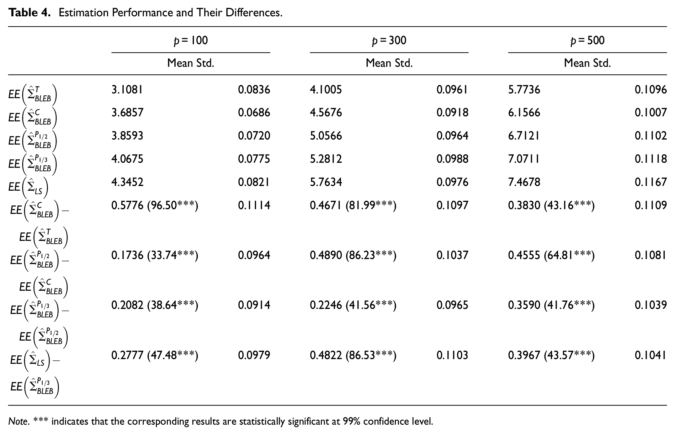
Table 4 reports the estimation performance of the five covariance matrix estimators when $n=100$ , $M=1000$ , and the number of assets $p$ is set to 100, 300, and 500. The reported average estimation error and associated standard errors are based on 1,000 simulations. The pair-wise differences of the estimation performance of the five estimators are also reported, along with the corresponding t-statistics.

Table 4.

Estimation Performance and Their Differences.

	p = 100		p = 300		p = 500
	Mean Std.		Mean Std.		Mean Std.
$\mathrm{EE}\left({\hat{\mathrm{\Sigma }}}_{\mathrm{BLEB}}^T\right)$	3.1081	0.0836	4.1005	0.0961	5.7736	0.1096
$\mathrm{EE}\left({\hat{\mathrm{\Sigma }}}_{\mathrm{BLEB}}^C\right)$	3.6857	0.0686	4.5676	0.0918	6.1566	0.1007
$\mathrm{EE}\left({\hat{\mathrm{\Sigma }}}_{\mathrm{BLEB}}^{P_{1/2}}\right)$	3.8593	0.0720	5.0566	0.0964	6.7121	0.1102
$\mathrm{EE}\left({\hat{\mathrm{\Sigma }}}_{\mathrm{BLEB}}^{P_{1/3}}\right)$	4.0675	0.0775	5.2812	0.0988	7.0711	0.1118
$\mathrm{EE}\left({\hat{\mathrm{\Sigma }}}_{\mathrm{LS}}\right)$	4.3452	0.0821	5.7634	0.0976	7.4678	0.1167
$\begin{array}{c}\mathrm{EE}\left({\hat{\mathrm{\Sigma }}}_{\mathrm{BLEB}}^C\right)-\hfill \\ \mathrm{EE}\left({\hat{\mathrm{\Sigma }}}_{\mathrm{BLEB}}^T\right)\hfill \end{array}$	0.5776 (96.50***)	0.1114	0.4671 (81.99***)	0.1097	0.3830 (43.16***)	0.1109
$\begin{array}{c}\mathrm{EE}\left({\hat{\mathrm{\Sigma }}}_{\mathrm{BLEB}}^{P_{1/2}}\right)-\hfill \\ \mathrm{EE}\left({\hat{\mathrm{\Sigma }}}_{\mathrm{BLEB}}^C\right)\hfill \end{array}$	0.1736 (33.74***)	0.0964	0.4890 (86.23***)	0.1037	0.4555 (64.81***)	0.1081
$\begin{array}{c}\mathrm{EE}\left({\hat{\mathrm{\Sigma }}}_{\mathrm{BLEB}}^{P_{1/3}}\right)-\hfill \\ \mathrm{EE}\left({\hat{\mathrm{\Sigma }}}_{\mathrm{BLEB}}^{P_{1/2}}\right)\hfill \end{array}$	0.2082 (38.64***)	0.0914	0.2246 (41.56***)	0.0965	0.3590 (41.76***)	0.1039
$\begin{array}{c}\mathrm{EE}\left({\hat{\mathrm{\Sigma }}}_{\mathrm{LS}}\right)-\hfill \\ \mathrm{EE}\left({\hat{\mathrm{\Sigma }}}_{\mathrm{BLEB}}^{P_{1/3}}\right)\hfill \end{array}$	0.2777 (47.48***)	0.0979	0.4822 (86.53***)	0.1103	0.3967 (43.57***)	0.1041

Note. *** indicates that the corresponding results are statistically significant at 99% confidence level.

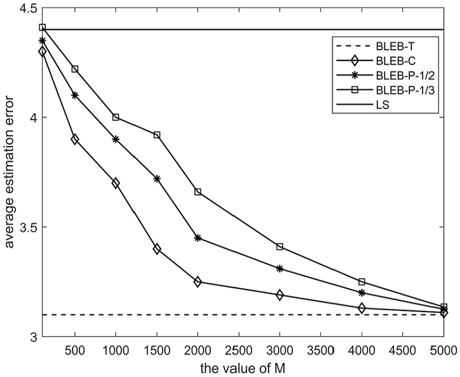
Figures 3 to 5 present the average estimation error of the five covariance matrix estimators when the number of assets $p$ is set to 100, 300, and 500, respectively. In each figure, we let $M$ grow from low to high to represent different accuracies of prior.

Figure 3.

Average estimation error with different M at p = 100.

Figure 4.

Average estimation error with different M at p = 300.

Figure 5.

Average estimation error with different M at p = 500.

From Table 4 and Figures 3 to 5, we can observe the following:

• The average estimation performance of the five estimators has the relationship $EE\left({\widehat{\mathrm{\Sigma }}}_{BLEB}^T\right)<EE\left({\widehat{\mathrm{\Sigma }}}_{BLEB}^C\right)<EE\left({\widehat{\mathrm{\Sigma }}}_{BLEB}^{P_{1/2}}\right)<EE\left({\widehat{\mathrm{\Sigma }}}_{BLEB}^{P_{1/3}}\right)<EE\left({\widehat{\mathrm{\Sigma }}}_{LS}\right)$

when $n=100$ , $M=1000$ at each $p$ of 100, 300, and 500. This result shows that the more information is used, the more accurate the estimator will be.

• The estimator ${\hat{\mathrm{\Sigma }}}_{\mathrm{BLEB}}^T$ performs the best since true prior of returns data has been used for estimation, although this is not achievable in practice. The estimator ${\hat{\mathrm{\Sigma }}}_{\mathrm{LS}}$ performs the worst because none of the prior information is considered. These results are consistent with Theorem 5.

• The estimator ${\hat{\mathrm{\Sigma }}}_{\mathrm{BLEB}}^C$ performs worse than ${\hat{\mathrm{\Sigma }}}_{\mathrm{BLEB}}^T$ since the estimated complete prior of returns data is inadequate. The estimator ${\hat{\mathrm{\Sigma }}}_{\mathrm{BLEB}}^C$ performs better than the estimator ${\hat{\mathrm{\Sigma }}}_{\mathrm{BLEB}}^{P_{1/2}}$ and ${\hat{\mathrm{\Sigma }}}_{\mathrm{BLEB}}^{P_{1/3}}$ since the former one has used more prior information for returns data, while this is not consistent with the conclusion that the BLEB estimator with complete data prior is equivalent to the BLEB estimator with partial data prior (full column rank case) in Theorem 5. This is because that the estimated data prior used in the simulation is different from the theoretical value of the data prior. However, the differences among ${\hat{\mathrm{\Sigma }}}_{\mathrm{BLEB}}^C$ , ${\hat{\mathrm{\Sigma }}}_{\mathrm{BLEB}}^{P_{1/2}}$ , and ${\hat{\mathrm{\Sigma }}}_{\mathrm{BLEB}}^{P_{1/3}}$ decrease with the increase of $M$ and they all converge on ${\hat{\mathrm{\Sigma }}}_{\mathrm{BLEB}}^T$ when $M$ is large enough. This is because that the estimated data prior gradually approaches to the theoretical value with the increase of $M$ . Clearly, the simulation results tell us that we should use estimated prior information as much as possible in practice.

• Figures 3 to 5 show that the average estimation errors of estimators ${\hat{\mathrm{\Sigma }}}_{\mathrm{BLEB}}^C$ , ${\hat{\mathrm{\Sigma }}}_{\mathrm{BLEB}}^{P_{1/2}}$ , and ${\hat{\mathrm{\Sigma }}}_{\mathrm{BLEB}}^{P_{1/3}}$ decrease with the increase of the value of $M$ . This makes good sense because the more accurate the estimated data prior is, the higher the estimation accuracy will be. This encourages us to discover more accurate data prior in practice as far as possible.

• The estimators ${\hat{\mathrm{\Sigma }}}_{\mathrm{BLEB}}^C$ , ${\hat{\mathrm{\Sigma }}}_{\mathrm{BLEB}}^{P_{1/2}}$ , and ${\hat{\mathrm{\Sigma }}}_{\mathrm{BLEB}}^{P_{1/3}}$ may perform worse than the estimator ${\hat{\mathrm{\Sigma }}}_{\mathrm{LS}}$ when $M=100$ (see Figures 4 and 5). This result indicates that the BLEB based covariance matrix estimators may lose efficacy when a extremely poor data prior is used for estimation.

Conclusions

In this paper, a class of BLEB estimation methods under the linear data model have been developed to improve the estimation accuracy in the case of unknown prior for the parameter. The proposed BLEB estimators perform better than the OWLS estimator since more data information is used to infer the parameter and they are equivalent to the LMMSE estimator when the complete or sufficient partial data prior is provided. Only when insufficient partial data prior is known is the MSE of the corresponding BLEB estimator larger than that of the LMMSE estimator, and it is still smaller than that of the OWLS method. A simple numerical example has been presented to verify the correctness of our method.

In addition, the estimation accuracy of high-dimensional covariance matrix using a factor model depends on the estimation accuracy of factor exposure or factor return. Therefore, we used the proposed BLEB estimator that fully considers the prior information of the data in this paper to estimate the high-dimensional covariance matrix, that is, we proposed the BLEB-based covariance matrix estimation method. Moreover, according to the different observable variables in the factor model, we given the specific implementation form of the BLEB method in two different cases of observable factor return and observable factor exposure. Finally, the simulation results also showed that the proposed BLEB-based method has a significant improvement in estimation accuracy compared with the traditional factor model method.

The works in this paper still have some limitations and need to be further studied in the future work. First, the BLEB-based high-dimensional covariance matrix estimation method is proposed in view of the shortcomings of the traditional factor model method. Therefore, this paper compares and analyzes the differences in the estimation accuracy of the two factor model based methods in detail, but we have not yet compared the performance differences between the BLEB method and other types of high-dimensional covariance matrix estimators. We will study this problem in future research. Second, in practical application, the BLEB method needs to first determine the prior mean and covariance of the return on assets. This paper has not yet discussed the possible impact of different prior estimators on the estimation results of the high-dimensional covariance matrix. In the future study, we will consider designing different prior of asset return, and analyze the impact of different prior on the actual estimation results.