Sage Journals: Discover world-class research

Abstract

This paper studies volatility scaling, a dynamic portfolio management method that maintains portfolio volatility at a target level over time. Analysis of U.S. equity returns shows that volatility scaling can generate unintended left-tail returns, negative returns not induced by the underlying asset, but by the act of scaling itself, particularly during periods of low portfolio volatility. To address this, this paper introduces a novel correction to volatility scaling in the form of a volatility floor. Using returns data from 1962 to 2018, this study compares a buy-and-hold portfolio, a volatility scaled portfolio, and a volatility scaled portfolio with a floor correction. Results show that introducing a volatility floor correction improves the left-tail of portfolio returns. With a volatility floor correction, the expected return below the first percentile of the volatility scaling strategy improves from −0.144 to −0.120, corresponding to an improvement of 0.024 in log returns. Robustness tests across subsamples (1962–1981, 1981–2000, 2000–2018) and pre-/post-Financial Crisis confirm these findings. Finally, the analysis highlights trade-offs between improving the left-tail and capping returns when implementing the volatility floor correction.

Plain Language Summary

Managing Volatility in Portfolios

Volatility scaling is a portfolio management method used to manage investment risks. This method is widely used by asset managers and has only recently received academic attention. The volatility scaling method scales any given portfolio over time to achieve a target level of risk that investors are comfortable with. This paper documents an unintended consequence of volatility scaling in generating large negative returns. These negative returns do not reflect the fundamental behavior of the asset, but are instead induced by the act of scaling. In order to correct this, this paper proposes a correction in the form of a volatility floor. By implementing this correction, this paper concludes that a volatility scaled portfolio with a floor correction results in a smaller left-tail of returns than a volatility scaled portfolio without such a correction. This is an important improvement over the state-of-the-art risk management strategy.

Keywords

volatility scaling portfolio management risk management

Introduction

Investors use active portfolio management to optimize for risk-adjusted portfolio performance. Among the approaches developed for this purpose, volatility scaling is one of the most popular portfolio management strategies for dynamically managing risk over time (Daniel & Moskowitz, 2016; Roncalli, 2016). The econometrics of such a strategy have only recently been formalized, motivating a surge in academic interest on the topic (Bai et al., 2023; Harvey et al., 2018; Poirier, 2021; Stewart et al., 2019). In this paper, we identify a drawback of the volatility scaling strategy and propose a correction to the strategy in the form of a volatility floor.

Volatility scaling is important to study for multiple reasons. First, this form of portfolio management provides an alternative to the traditional risk-management method of diversification (Ghosh, 2010; Hocquard et al., 2013). For example, an investor may choose to invest across sectors or asset classes to reduce the risk that a downturn in one particular sector or class dominates portfolio performance. However, during crisis, historical correlations between asset classes and their volatility characteristics often break down (Hamill et al., 2016). The phase-locking behavior of assets in crisis, combined with sharp increases in market volatility, may lead to substantial losses for portfolios relying solely on traditional diversification (Naeem et al., 2023). As a result, volatility scaling has gained traction as an alternative means of managing downside risk, particularly during periods of extreme returns (Shiraz et al., 2020; Tavana et al., 2019).

To contextualize volatility scaling in the broader landscape of portfolio management strategies, we further note that this strategy is designed to dynamically adjust the notional exposure of an investor’s portfolio. For example, volatility scaling helps investors decrease risk exposure when volatility is high and increase risk exposure when volatility is low. This strategy shares similar mechanisms with momentum trading for the reason that the timing of position adjustments introduced by volatility scaling imposes a “leverage effect” on the underlying returns (Harvey et al., 2018).

Given the usage of volatility scaling as a strategy to manage downside risk, the goal of this paper is to document a drawback of the volatility scaling method and to propose a solution. First, we identify the drawback of volatility scaling in generating left-tail returns that would otherwise not exist in a static buy-and-hold portfolio. Second, we propose a correction to volatility scaling in the form of a volatility floor. Under this correction, when the overall portfolio volatility is equal to or exceeds the volatility floor, the strategy is identical to the standard volatility scaling strategy. However, when the overall portfolio volatility falls below the volatility floor, scaling is based on the volatility floor rather than the observed volatility. As such, the volatility floor correction maintains the dynamic nature of the volatility scaling strategy, while imposing a bound on the degree of scaling in low-volatility regimes.

Our main findings support our hypothesis that introducing a volatility floor correction outperforms the state-of-the-art volatility scaling strategy without such a correction. Using stock returns from the Wharton Center for Research in Security Prices (CRSP) Index File over 14,221 trading days, we show that a volatility scaled portfolio generates lower average returns below the first and fifth percentile than the static buy-and-hold portfolio. Incorporating a volatility floor correction reduces the left-tail outcomes. Over the time period 1962 to 2018, the expected return below the first percentile is −0.120 for the floored portfolio, compared with −0.144 for the volatility scaled portfolio without a floor correction, corresponding to an improvement of 0.024 in log returns. Similarly, the expected return below the fifth percentile for the floored portfolio improves by 0.022 in log returns relative to the volatility scaled portfolio without a floor correction. These findings are robust across different subperiods and market regimes.

Our finding that volatility scaling generates an unintended left-tail has important implications for investors pursuing such a strategy. Typically, investors who choose to implement the volatility scaling strategy are those who prioritize safeguards in managing their portfolios and in generating stable returns (Barroso & Santa-Clara, 2015). These investors, such as insurance companies and pension funds, prioritize risk management. As such, volatility scaling induced left-tail events are contrary to the goals of these investors when implementing such a strategy.

Given our main findings, our contribution to the literature is as follows. First, while there is a vast body of literature on portfolio management methods, there is sparse literature on volatility scaling. The discussion around this particular portfolio management strategy is guided by a few pieces of recent publications, and this paper seeks to add to the growing body of research by documenting the unintended consequence of volatility scaling. Second, while prior empirical literature has mostly focused on assessing the volatility scaling methodology by comparing its performance with unscaled portfolios, the current paper introduces a novel correction to the method, in addition to assessing its performance. The findings of this paper have important implication for the implementation of volatility scaling or related volatility targeting strategies in practice. Namely, we recommend risk-averse practitioners to implement a volatility floor correction to the volatility scaling strategy to protect against left-tail risk during low volatility periods.

This paper is organized as follows. The Literature Review Section discusses related work. The Data and Methods Section introduces the portfolio construction methodologies. The Results Section presents the main findings of the paper. The Discussion and Implications Section discusses robustness and trade-offs. The Conclusion Section summarizes the main conclusions and suggests next steps.

Literature Review

Volatility Scaling as a Portfolio Management Strategy

There is a wealth of literature on portfolio management strategies for the active investor. Broadly, these strategies fall into two streams of literature. The first stream of literature focuses on alpha generating strategies, while the second stream of literature focuses on defensive strategies (Haddad et al., 2020; Munir et al., 2022). While volatility scaling is a relatively new insurance strategy, earlier forms of risk management in the same spirit can be traced to the use of options to hedge a given portfolio (Brennan & Schwartz, 1989). Although options remain a common tool for hedging volatility, investors are cautious about the costs associated with such portfolio management methods (Dopfel & Ramkumar, 2013; Maillard et al., 2010). Hedging via options to limit risk exposure, when compared with volatility scaling, tend to be more costly to maintain. Involving options also lead to more complicated considerations for investors such as the need to hedge first- or second-order greeks. As such, volatility scaling has emerged as a preferred way of delivering the same level of dynamic portfolio management (Hocquard et al. 2013).

While volatility scaling is related to widely studied portfolio strategies such as volatility-weighting, the literature has drawn clear distinctions between the two. One important characteristic of the volatility scaling strategy is its emphasis on allocating risk equally across time, rather than across portfolio constituents (Molyboga, 2020). Consider an investor with a given risk target holding a portfolio of various assets. If market conditions change and the assets become more volatile, and thus more risky to hold, the risk associated with the portfolio will exceed the investor’s risk target. This implies that the original holdings of assets will no longer be optimal given the investor’s preferences. Volatility scaling prescribes that the investor scale down holdings such that the overall volatility of the portfolio returns to the desired risk level. In this way, volatility scaling is a dynamic portfolio management method that adjusts as portfolio risk evolves.

Given the empirical importance of volatility scaling as a portfolio management strategy, Hoyle and Shephard (2018) formalize the econometrics of volatility scaling, also referred to as dynamic risk parity. In their paper, Hoyle and Shephard detail the properties of volatility scaling by relating the sequence of returns to $\frac{1}{σ_{t}}$ , termed the root precision process. They conclude with two important theorems, one describing the expected sequence of returns under the volatility scaled position and the other describing the unconditional Sharpe improvement as a function of volatility.

A related literature discusses how to best model portfolio volatility. Dachraoui (2018) points out that the usefulness of the volatility scaling method is conditional on both how volatility is estimated and on the volatility target itself. Barroso and Santa-Clara (2015) model volatility using an Autoregressive (AR(1)) model. Daniel and Moskowitz (2016) incorporate a Generalized Autoregressive Conditional Heteroskedasticity (GARCH) model, as do Moreira and Muir (2017), Hoyle and Shephard (2018), and Di Persio et al. (2021). In our paper, we follow the existing literature in the choice of models for portfolio volatility. To further address concerns that the usefulness of volatility scaling is conditional on the volatility target, we conduct robustness tests by varying volatility targets and by examining the performance of portfolios over subperiods with non-overlapping returns.

Evaluation of Volatility Scaling in Practice

Albeverio et al. (2013) and Hocquard et al. (2013) first formally show the benefits of managed volatility relative to traditional hedging methods by analyzing a constant volatility framework. Albeverio et al. (2013) highlight the fact that equity volatility is not constant and use this to motivate the need for maintaining a constant volatility to dampen the impact of market correction. Hocquard et al. (2013) use a similar motivation to show that a constant volatility strategy on a Canadian pension fund proxy portfolio outperforms the baseline portfolio with non-constant volatility. Importantly, Hocquard et al. (2013) also establish cumulative returns as an evaluation metric for comparing the performance of the constant volatility strategy against a non-constant volatility portfolio. Furthermore, they show that the constant volatility strategy outperforms strategies which solely rely on diversification as a portfolio management tool.

Following findings formally establishing the benefits of volatility managed portfolios in practice, the literature turns to different methods of measuring portfolio performance and evaluating the performance of the strategy across asset classes. For example, as opposed to using cumulative returns as an evaluation metric, Perchet et al. (2015) use simulation methods in order to address the draw-back of having limited realized returns data. Using simulated data across asset classes, Perchet et al. (2015) find that volatility scaling is the most effective when applied to equities because equities exhibit large tails in returns and exhibit a strong negative relationship between returns and volatility, compared to other asset classes such as treasuries. As such, Perchet et al. (2015) suggest that volatility scaling is best applied to and analyzed within the equities asset class. Given the existing evidence demonstrating the effectiveness of volatility scaling for equities, this paper is motivated to examine any unintended consequences of the volatility scaling strategy within this asset class.

More recently, the literature has converged on a set of metrics to better evaluate the volatility scaling strategy relative to other strategies. For example, following Perchet et al. (2015), Harvey et al. (2018) similarly assess the performance of volatility scaling across different industries and asset classes using realized returns. The authors use mean shortfall and mean exceedance, in addition to the Sharpe, to compare the performance of the volatility scaling with non-scaled portfolios. Given the precedent of using these metrics, this paper similarly reports these measures for the volatility floored portfolio. Furthermore, Harvey et al. (2018) perform robustness tests by evaluating the performance of volatility scaling on ten industry portfolios, in addition to U.S. equities and fixed income portfolios. Similarly to Perchet et al. (2015), Harvey et al. (2018) conclude that volatility scaling can help boost Sharpe ratios when assets comprising the portfolio are more risky. This conclusion makes intuitive sense as less risky methods require less scaling for the investor to maintain the same target risk level. The conclusion from Harvey et al. (2018)’s survey of asset classes motivates the focus on this paper on the S&P 500 Equity Index.

Research Gaps and Hypothesis Formation

Our paper relates to the prolific literature studying the broad properties of volatility. For instance, existing papers establish the negative relationship between volatility and returns and empirically show that this combination of high vol-low return property of asset prices are often realized during bear market regimes and depends on the nature of the trading day (Chen et al., 2022; Cui et al., 2023; Just & Echaust, 2020). This provides evidence that a dynamic portfolio management method must take into account the interaction between volatility and returns and the implications of scaling under different volatility environments.

While the traditional volatility scaling method manages risk well precisely during these high vol-low return environments, absent from the literature is a clear characterization of the volatility scaling strategy during low volatility regimes. Our paper fills this gap in the literature by documenting how the volatility scaling strategy performs over time. Our paper contributes by identifying conditions under which returns are amplified by volatility, highlighting the role of volatility–return correlation as a mechanism underlying the performance of volatility scaling strategies.

In our paper, in addition to documenting the tendency of volatility scaling to generate large, unintended negative returns, we propose a correction to volatility scaling in the form of a volatility floor. To contextualize our findings in existing literature, we combine the performance statistics used in Hocquard et al. (2013) and Harvey et al. (2018) and include an additional performance metric to evaluate the fifth percentile of returns for various portfolios. In proposing a volatility floor correction and comparing the corrected portfolio with the standard volatility scaled portfolio, this paper fills a vacancy in existing literature by documenting the extent to which a volatility floor correction mitigates a large left-tail of the return distribution.

We propose the following testable hypothesis:

H1. Volatility scaling outperforms the buy-and-hold portfolio on average.

H2. Volatility scaling generates unintended negative returns, particularly during periods of low volatility.

H3. Volatility scaling with a volatility floor correction mitigates the unintended negative returns induced by the scaling strategy.

Data and Methods

In this section, we begin by defining the three types of portfolios considered in this paper: the static buy-and-hold portfolio, the dynamic volatility scaled portfolio, and the volatility scaled portfolio with a floor correction and then discuss the empirical strategies used to test the hypotheses above.

Static Buy-and-Hold Portfolio

We obtain daily S&P Composite Index price data from the Wharton Center for Research in Security Prices (CRSP) Index File. We compute daily returns using price levels excluding dividends recorded at the end of each trading day. The resulting returns represent the change in the values of the component securities underlying the S&P index. For a static buy-and-hold portfolio, we assume the investor holds the S&P Composite Index over our sample from 1962 to 2018.

For a static investor, the daily return of a buy-and-hold portfolio at time t is given by:

Y_{t} = \ln (\frac{{SPINDX}_{t}}{{SPINDX}_{t - 1}})

(1)

where $SPIND X_{t}$ denote the level of the S&P Composite Index on trading day t.

Figure 1 plots the time-series of $Y_{t}$ over our sample period, which shows how returns have varied for a buy-and-hold investor. Note that for such an investor, portfolio returns vary widely around market-moving events such as Black Monday and the Financial Crisis. This motivates the volatility scaling approach, which attempts to limit the amount of losses resulting from such large variations in price levels of a static, unscaled portfolio. Furthermore, Figure 1 shows that when a left-tail event such as the Financial Crisis takes place, companies in the index tend to move in the same direction, corroborating the finding that managing risk by simply investing across industries does not serve as a sufficient safeguard for returns (Barroso and Santa-Clara, 2015).

Figure 1.

Daily returns of the static buy-and-hold portfolio.

Figure 2 shows the cumulative returns of an investor who holds the static, unscaled portfolio from 1962 to the end of our sample period using the definition of daily returns as in Equation 1. We observe that compared with daily returns recorded in Figure 1, large fluctuations in daily returns of the S&P index generally correspond to dip in the cumulative returns of the portfolio. This is in accord with the general understanding that high volatility correlates with negative returns (Fleming et al., 2001, 2003).

Figure 2.

Cumulative returns of the static buy-and-hold portfolio.

Dynamic Volatility Scaled Portfolio

For a volatility scaled portfolio, we adjust our position on a daily basis such that our position delivers the same amount of risk. For example, if the target volatility level is 15%, and the volatility of our portfolio is below target level, we will scale up our position. By adjusting our holdings, we realize a constant level of exposure to volatility. In computing daily returns for a volatility scaled portfolio, let $σ_{target}$ denote the annualized target portfolio volatility and $σ_{t}$ denote estimated volatility at time t. We calculate the daily returns for a volatility scaled portfolio, $Y_{σ}$ , as

\begin{matrix} Y_{t} = \ln (\frac{SPIND X_{t}}{SPIND X_{t - 1}}) \end{matrix}

(2)

In our returns analysis, we further partition our data into three consecutive time periods to better examine trends underlying the overall available data. We construct the time period divisions as naturally as possible by simply creating three periods that contain an equal number of data points. Conveniently, doing so isolates major market events such as the burst of the dot-com bubble and the Financial Crisis. This method of time-partitioning also ensures that the each period contains a sufficient number of observations for our analysis. Doing so yields the partition of the overall time period into 1962 to 1981, 1981 to 2000, and 2000 to 2018.

As an additional robustness check, we repeat our analysis by further partitioning the sample period into distinct market regimes as partitioned by the Financial Crisis. We separately examine portfolio returns pre-December 2007 and post-December 2007, where the cutoff date is determined by the start date of the NBER recession time period.

To show that our results are invariant to the modeling choices for $σ_{t}$ , we use two methods to estimate variance, $σ_{t}^{2}$ , both of which are widely used in literature and in industry. The first model is the moving average model. We choose the time horizon of the model to be the trailing twelve trading days. We estimate variance at time t based on realized returns from t−12 to t−1. Given the choice of using a MA(12) model, we would expect to see slightly larger magnitudes of scaling given that the estimated volatility will exhibit more fluctuations than if we choose to use a longer period of trailing data to inform our volatility estimate (Dachraoui, 2018).

Using this model, $σ_{t}$ is estimated by the square root of

\begin{matrix} σ_{t}^{2} = \frac{Y_{t - 1}^{2} + \dots + Y_{t - 12}^{2}}{12} \end{matrix}

(3)

We plot resulting estimates of $σ_{t}$ for the period of 1962 to 2018. We make the following observations. The time period pre-1981 is the relatively low volatility regime, with no major spikes in volatility when compared with the large spike in volatility in the late 1980s and the early 2000s. The time period from 1981 to 2000 captures at least one large volatility spike. The time period after 2000 captures the burst of the tech bubble and the Financial Crisis. Based on the volatility estimates over time, H2 suggests that we should observe a worse performance from the volatility scaling strategy relative to the baseline buy-and-hold strategy in the subsample prior to 1981, given this was a period of low volatility. H3 suggests that we should see improvements in the left-tail of returns if the volatility floor correction is introduced (Figure 3).

Figure 3.

Daily volatility estimates using the moving average MA(12) method.

In order to ensure that we capture the structure of volatility in financial markets, we report the results in this paper using the integrated GARCH model as the preferred specification for portfolio volatility. Following Hoyle and Shephard (2018), we model volatility using an integrated GARCH model with 12-day half-life. By inspecting the time-dependencies of the data by plotting autocorrelation and partial autocorrelation graphs for the log returns, residuals, and the square of residuals, we employ the GARCH(1,1) model as our preferred model specification. Using this model allows us to capture both the short-term correlation and the long-run mean reversion, two specific volatility features (Hocquard et al., 2013). We continue by building a GARCH model in the form of

\begin{matrix} σ_{t}^{2} = α σ_{t - 1}^{2} + {β Y}_{t - 1}^{2} \end{matrix}

(4)

We impose the constraint that $α + β = 1$ . Table 1 reports the results from fitting the model.

Table 1.

Regression Output from the GARCH (1,1) Model of Volatility.

Variables	Coefficient	Standard error
α	0.0776	0.006203
β	0.9201	0.006042

Table 1 suggests that daily volatility estimates are highly dependent on historical portfolio volatility. The 0.92 coefficient estimate reflects the realistic observation of volatility regimes documented in literature while the non-zero coefficient in front of $Y_{t - 1}^{2}$ reflects the correlation between portfolio volatility and past squared returns. As such, we carry out all following analysis using the $σ_{t}$ approximation given by

\begin{array}{l} σ_{t}^{2} = 0.92 σ_{t - 1}^{2} + 0.08 Y_{t - 1}^{2}, \\ t = 1, 2, \dots, T \end{array}

(5)

This is our preferred specification for $σ_{t}^{2}$ as it appears in Equation 2 when used as the baseline portfolio volatility used for volatility scaling.

Volatility Scaled Portfolio with a Floor Correction

In order to determine the appropriate volatility floor, we estimate a logistic regression to categorize whether left-tail returns that appear in the returns of the volatility scaled portfolio, but not the static portfolio, are driven by periods of low volatility. To do so, we focus on negative returns which would not have occurred without volatility scaling, but did occur due to volatility scaling magnifying the negative returns of the underlying portfolio. Henceforth, we denote these as “red events.”

Let Y be a binary variable denoting whether an event is a red event or not. That is, $Y = 1$ if an event is classified as yielding returns lower than $p_{1}$ only for the dynamic portfolio, and $Y = 0$ if otherwise. We are thus interested in modeling

P (Y = 1 | σ)

We record the volatility level σ which minimizes the mis-classification rate. That is, we record the volatility level such that if we predict $Y = 1$ when $σ_{t} < σ$ and $Y = 0$ when $σ_{t} > σ$ , we classify red events with the greatest accuracy. This serves as the candidate for the level d of the volatility floor portfolio. We perform our analysis on both testing and training sets, using a 70-30 split of our overall sample, and we select the volatility level σ which delivers the highest classification accuracy for red events.

Note that we are less concerned with fine-tuning the predictive power of the model. This is because our focus is not on the exact probability of an event being a “red event” based on the GARCH-modeled volatility for a specific day. Rather, we are concerned with isolating the GARCH-modeled volatility variable and determining the ability of this single variable in delineating between two states of portfolio performance. Thus, it suffices for our purpose to use simple regression methods. If the GARCH-modeled volatility can differentiate between red and non-red events, we would expect to see a clear distinction between red and non-red events when plotted against volatility. Otherwise, we would not expect to see a clear delineation.

Imposing a volatility floor controls how much the dynamic investor will scale up their position in periods of low volatility. Consider a hypothetical investor who applies the volatility-scaling strategy with a volatility floor. Denote the value of the volatility floor as d. A volatility scaled portfolio with a floor correction is constructed as follows

Model $σ_{t}$ for all days t using the previously defined GARCH model

Volatility scale holdings using $σ_{t}$ for $σ_{t} > d$

Volatility scale holdings using d for $σ_{t} \leq d$

Daily returns in Step 2 are computed as previously defined,

\begin{matrix} Y_{σ} = Y_{t} \frac{σ_{target}}{σ_{t}} \end{matrix}

(6)

Daily returns in step 3 are computed with the updated floor volatility $d,$

\begin{matrix} Y_{σ} = Y_{t} \frac{σ_{target}}{d} \end{matrix}

(6)

We compare the performance of the volatility scaled portfolio with a floor correction with the static buy-and-hold portfolio and the dynamic volatility scaled portfolio using the metrics reported in Table 2.

Table 2.

A List of Performance Statistics Used to Compare Portfolios Under Consideration.

Variable	Variable name	Variable definition
$SR$	Sharpe ratio	Ratio of the mean and standard deviation of returns, annualized
$\bar{R}$	Mean returns	Expected daily returns on a log scale
$R_{σ}$	Standard deviation of returns	Standard Deviation as modeled using the GARCH model
$p_{1}$	First percentile cutoff	First percentile of daily returns of a portfolio holding, representing the extreme left-tail
$p_{5}$	Fifth percentile cutoff	Fifth percentile of daily returns of a portfolio holding, representing the extreme left-tail
$Los s_{p 1}$	First percentile average loss	Mean of returns below the first percentile, found by first calculating $p_{1}$ and taking the subpopulation of returns less than $p_{1}$
$Los s_{p 5}$	Fifth percentile average loss	Mean of returns below the fifth percentile, found by first calculating $p_{5}$ and taking the subpopulation of returns less than $p_{5}$

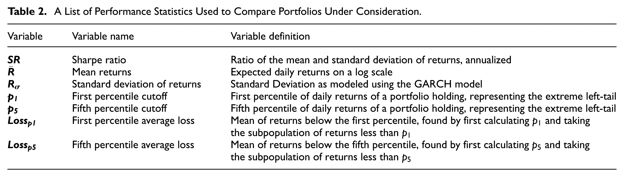
The performance statistics as defined in Table 2 test the hypotheses of the paper in the following ways. The statistics $p_{1}$ , $p_{5}$ , $Los s_{p_{1}}$ , and $Los s_{p_{5}}$ capture the left-tail of the distribution of returns. Of these, a more negative $p_{1}$ or $p_{5}$ corresponds to a more extreme left-tail. A more negative $Los s_{p_{1}}$ or $Los s_{p_{5}}$ corresponds to a lower expected return, conditional on being in the left-tail as defined by percentile cutoffs. When comparing across strategies, a higher Sharpe Ratio or a higher average return of the volatility scaling strategy compared with the static buy-and-hold strategy would support H1. More negative left-tail statistics of the volatility scaling strategy compared with the static buy-and-hold strategy, particularly in low portfolio volatility environments, would support H2. Finally, an improvement in the left-tail statistics of the volatility scaling strategy with a floor correction when compared with the volatility scaling strategy without such a correction would support H3 that introducing a volatility floor correction mitigates the left-tail risk induced by the scaling strategy itself.

Results

In the results section, we first compare the performance of the static and dynamic portfolios. We then highlight the drawbacks of the dynamic portfolio management strategy and use these findings to motivate the volatility floor. Finally, we compare the performance of the floored portfolio with the dynamic portfolio.

Returns Comparison Analysis

In this section we compare the performance of the static versus dynamic portfolio by analyzing daily returns. Figure 4 shows the comparison of daily returns for the dynamic versus the static portfolio from 1962 to 2018. The time-series returns of the static portfolio, which provides the baseline for comparison, are shown in blue, and the time-series returns of the dynamic portfolio are shown in red. The three panels of the figure correspond to dynamic portfolios held by investors with different volatility targets, $σ_{target} = {10 %, 15 %, 20 %}$ .

Figure 4.

Daily returns of the static versus dynamic portfolios with different levels of volatility targets. The top, middle, and bottom figures correspond to volatility targets of 10%, 15%, and 20%, respectively.

Figure 4 illustrates that the performance of the dynamic portfolio depends on the choice of volatility target. For example, the bottom panel of Figure 4 shows that a dynamic portfolio with $σ_{target} = 20 %$ generates more negative daily returns than the static portfolio. This suggests that maintaining a volatility target of $20 %$ is likely not a meaningful portfolio management strategy for an investor attempting to minimize left-tail of returns. However, around extreme left-tail inducing events such as Black Monday (1987), the bear market of 1974, and the Financial Crisis (2008), the static portfolio underperforms the dynamic portfolio regardless of the target volatility selected. Thus, the time-series comparison of daily returns suggests that for an investor employing a static portfolio management strategy, volatility scaling would provide return protection during extreme events.

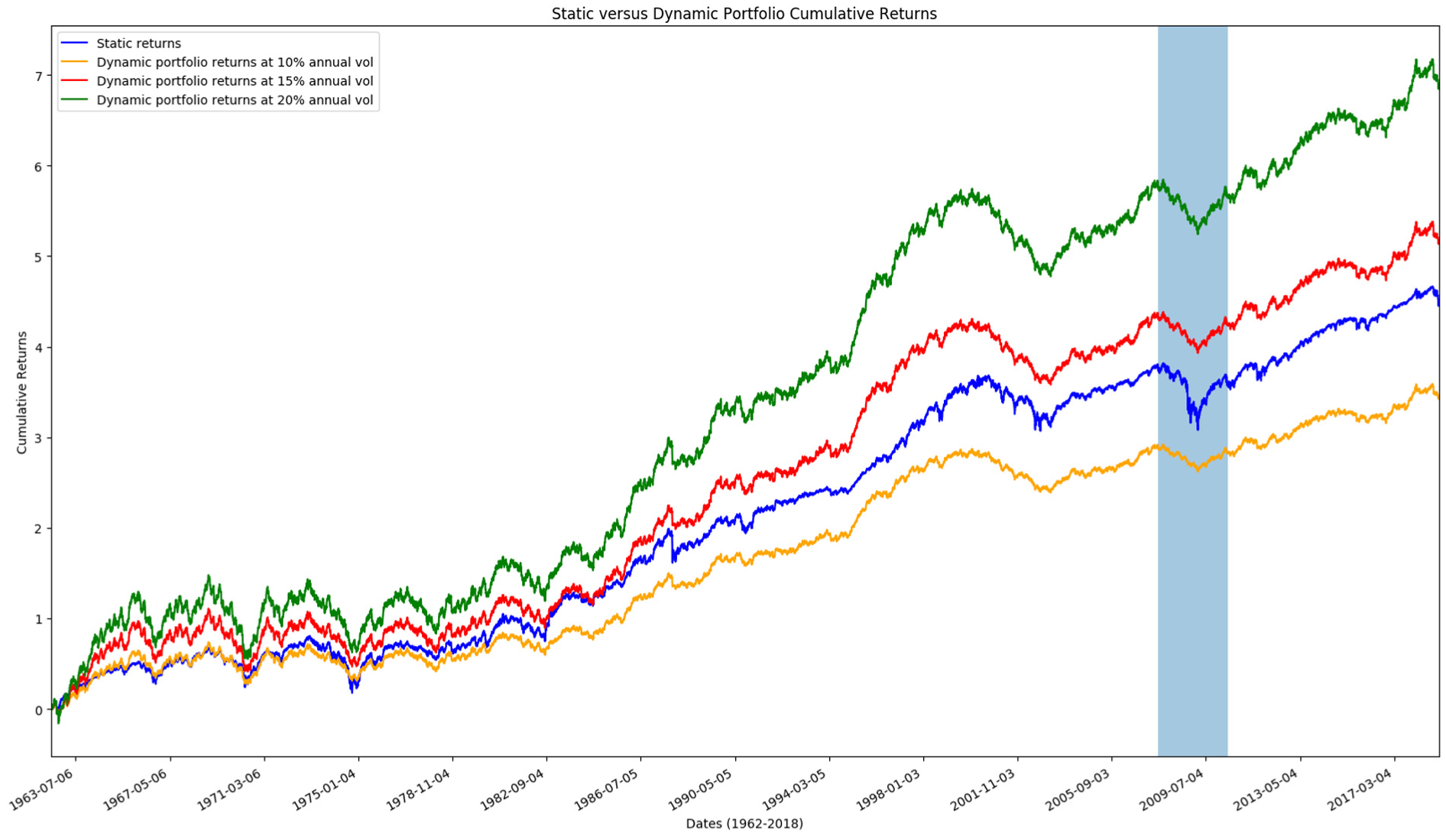
We similarly compare the cumulative returns of the static portfolio versus the dynamic portfolio with volatility targets $σ_{target} = {10 %, 15 %, 20 %}$ in Figure 5. That is, we examine the returns of the hypothetical investor assuming they initiated their position in 1962 and maintained their position, via either static or dynamic methods, until 2018. Blue denotes the baseline static portfolio. Yellow, red, and green denote $σ_{target} = {10 %, 15 %, 20 %}$ annual volatility targets respectively. The blue shaded area corresponds to the Financial Crisis to illustrate the performance of the four different portfolios during a black swan event.

Figure 5.

Cumulative returns of the static versus dynamic portfolios with different levels of volatility targets.

Changes in cumulative returns around the Financial Crisis as shown in Figure 5 corroborate our earlier finding that during events that causes the entire market to sell-off, the static portfolio suffers a significant drop in returns relative to the dynamic portfolio, regardless of the volatility target selected. During this same period, a dynamic portfolio with $σ_{target} = 10 %$ experienced the least amount of losses. However, we note that the cumulative returns of the $σ_{target} = 20 %$ portfolio is significantly higher than the cumulative returns of all other portfolios over our sample period. In fact, the dynamic portfolio with a $10 %$ annual volatility target offered the highest degree of protection during the Financial Crisis, but yielded the lowest amount of cumulative returns over the entire time period.

In order to reconcile such trade-off between risk (volatility) and reward (returns), we report summary statistics for the performance of the static and dynamic portfolios in Table 3. We elect to report summary statistics in the form of monthly returns to reflect the observation that in practice, investors are unlikely to hold a portfolio across our entire sample period (1962–2018) and are more likely to review the performance of their portfolios on a monthly or quarterly basis. We observe that the volatility scaled portfolio results in a larger Sharpe ratio and larger mean returns relative to the benchmark portfolio for the time period of 1962 to 2018. The portfolio of the dynamic investor has a Sharpe ratio of 0.457 and the portfolio of the static investor has a Sharpe ratio of 0.437. This comparison supports our hypothesis H1 and suggests that more returns is generated per unit of risk for the dynamic portfolio than the static portfolio.

Table 3.

Descriptive Statistics of Monthly Portfolio Returns.

	Performance metrics			Left tail metrics
Portfolio Type	SR	$\bar{R}$	$R_{σ}$	$p_{1}$	$Los s_{p 1}$	$p_{5}$	$Los s_{p 5}$
Static portfolio	0.437	0.005	0.044	−0.127	−0.179	−0.068	−0.106
Dynamic portfolio	0.457	0.006	0.049	−0.123	−0.144	−0.079	−0.106

Note. SR denotes the Sharpe Ratio. $\bar{R}$ denotes average returns. $R_{σ}$ denotes the standard deviation of returns. $p_{1}$ denotes the first percentile return cutoff. $Los s_{p 1}$ denotes the average return below the first percentile return cutoff. $p_{5}$ denotes the fifth percentile return cutoff. $Los s_{p 5}$ denotes the average return below the fifth percentile return cutoff.

In order to test H2, we report differences in the left-tail of the return distribution in the left panel of Table 3. Recall that $p_{x}$ denotes the x percentile returns threshold and $Los s_{p_{x}}$ denotes the average of all returns that fall below $p_{x}$ . A less negative $p_{1}$ for the dynamic portfolio of −0.123 indicates that the lowest 1% of returns for the dynamic portfolio represent smaller losses than the lowest 1% of returns for the static portfolio. A comparison of $Los s_{p_{1}}$ for the two portfolios corroborates this observation. However, the reverse is observed for $p_{5}$ , where the static portfolio has a less negative percentile threshold, but nonetheless results in an expected loss similar to that of the dynamic portfolio. The relationship between $p_{1}$ and $p_{5}$ of the static and dynamic portfolios suggests that while volatility scaling improves the extreme left-tail events, it introduces unintended consequences. Namely, we document that over the time period of 1962 to 2018, the dynamic portfolio management strategy generates a larger left-tail than the static portfolio when the left-tail is measured using the lower fifth percentile of returns. This result is in line with the research objective of illustrating the unintended consequences of a scaling strategy and provides evidence for H2. While volatility scaling is intended to help investors manage the risk of their portfolios, Table 3 suggests that this method can be improved upon to achieve its objectives. We thus propose a correction to volatility scaling and illustrate its validity in Section 4.3.

Subsample Analysis

In this section, we discuss unintended consequences of the state-of-the-art volatility scaling method across subsamples. Table 4 reports descriptive statistics of returns over the sample periods 1962 to 1981, 1981 to 2000, and 2000 to 2018. Comparing the Sharpe Ratio of the static and dynamic portfolio with fixed $σ_{target} = 15 %$ over the three subsamples reveal that the dynamic portfolio generates a higher Sharpe Ratio than the static portfolio in time periods 1981 to 2000 and 2000 to 2018, but generates lower returns per unit of risk for the time period 1962 to 1981. While summary statistics from Table 3 demonstrates that the dynamic portfolio generates a higher Sharpe Ratio for the overall period, Table 4 shows that this is largely driven by the larger magnitude in the differences in Sharpe ratios for the latter two time periods. The dynamic investor from 1981 to 2000 outperforms the static investor by 0.035 in Sharpe, and the dynamic investor from 2000 onwards similarly outperforms the static investor by 0.088. In comparison, the dynamic investor underperforms the static investor in both Sharpe and average returns from 1962 to 1981.

Table 4.

Descriptive Statistics of Monthly Portfolio Returns Across Three Subsample Periods.

Static
	Performance metrics			Left tail metrics
Sample Period	SR	$\bar{R}$	$R_{σ}$	$p_{1}$	$Los s_{p 1}$	$p_{5}$	$Los s_{p 5}$
1962–1981	0.275	0.003	0.044	−0.121	−0.140	−0.069	−0.098
1981–2000	0.918	0.011	0.049	−0.089	−0.173	−0.055	−0.089
2000–2018	0.199	0.003	0.047	−0.152	−0.206	−0.078	−0.124
Dynamic
	Performance metrics			Left tail metrics
Sample Period	SR	$\bar{R}$	$R_{σ}$	$p_{1}$	$Los s_{p 1}$	$p_{5}$	$Los s_{p 5}$
1962–1981	0.253	0.004	0.057	−0.138	−0.150	−0.096	−0.121
1981–2000	0.953	0.013	0.046	−0.109	−0.140	−0.064	−0.092
2000–2018	0.287	0.003	0.042	−0.104	−0.124	−0.073	−0.092

A similar conclusion is drawn when comparing $p_{1}$ , the first percentile of returns, across static and dynamic portfolios in Table 4. While the first percentile of returns for the dynamic investor is less negative than that for the static investor for time periods 1981 to 2000 and 2000 to 2018, the first percentile for 1962 to 1981 is more negative for the dynamic profile by 0.27 on a log scale. This observation similarly holds for the expected loss of returns that fall under the fifth percentile. For metrics related to the fifth percentile, $p_{5}$ and $Los s_{p_{5}},$ the dynamic portfolio only outperforms the static portfolio from 2000 to 2018, the last subperiod.

Table 4 suggests that the volatility scaling method has varied impact on portfolio returns depending on the volatility environment. This observation is in accord with our hypothesis that under some market conditions, a constant volatility strategy negatively impacts returns. That is, by nature of the volatility scaling strategy, which scales up the portfolio during periods of low volatility and scales down the portfolio during periods of high volatility, the strategy may give rise to unexpected tail-events. This suggests that the relatively larger left tail of returns under the dynamic scaling strategy is not characteristic of the underlying index itself, but a result of scaling up during low-volatility regimes of returns.

We note that Tables 3 and 4 both corroborate the merit of the scaling strategy when using Sharpe as a metric. However, as we will show in the following section, a simple correction in the form of a volatility floor will exhibit significant improvements in the metrics used to measure the left-tail. Furthermore, we will show in the following section that this finding is robust to subsampling by market regimes, as opposed to equally dividing the sample period.

Performance of the Volatility Floor Correction

In this section we focus our analysis on the left-tail of returns, which are returns below the first percentile of all returns generated by a portfolio management strategy over our sample period. To directly test H2 that volatility scaling introduces unintended returns in low-volatility regimes, we compare the days on which left-tail returns are generated for the static and dynamic portfolios in Figure 6. The top, middle, and bottom panel represent time periods 1962 to 1981, 1981 to 2000, and 2000 to 2018, respectively. Within each panel, green points denote trading days on which the daily return falls below the first percentile of the static portfolio and below the first percentile of the dynamic portfolio. Yellow points denote trading days on which the daily return falls below the first percentile of the static portfolio, but above the first percentile of returns for the dynamic portfolio. Finally, red points denote trading days on which the daily return falls below the first percentile of the dynamic portfolio, but above the first percentile of returns for the static portfolio. These events are plotted on a time-series of portfolio volatility.

Figure 6.

Visualization of left-tail events across three subperiods from 1962 to 2018. Red events denote left-tail events that only appear within the dynamic portfolio. The first, second, and third panels correspond to 1962 to 1981, 1981 to 2000, and 2000 to 2018, respectively.

If volatility scaling does not introduce any additional left-tail events, we should not expect to see any red events in Figure 6. However, we observe multiple red events for all subsamples. That is, there are instances across all three subsamples where a left-tail event would not have occurred without volatility scaling, but did occur due to volatility scaling magnifying negative returns of the underlying asset. What is striking is the consistency in the position of the red events relative to the volatility of the portfolio. Across all three subsamples, we observe left-tail events occurring in low volatility regimes, as indicated by the y-axis. For example, from 1962 to 1981, all realization of returns below the first percentile of the dynamic portfolio, but above the first percentile for the static portfolio, with the exception of one daily return, occurred on days when the volatility of the underlying portfolio is below 0.10. For 1981 to 2000 and 2000 to 2018, this observation again holds true, but for a threshold volatility of 0.20. All left-tail events realized in the dynamic strategy were realized on days of low portfolio volatility. This finding provides strong evidence in support of our H2 that when volatility is low, the dynamic portfolio is prone to left-tail risk that do not exist in a static portfolio.

To establish statistical significance of the asymmetry in performance of the volatility scaling method under different volatility regimes, we next present regression results from logistic and linear regressions. Figure 7 plots the model fit of using portfolio volatility to predict the probability of a red event, an instance where the portfolio return falls under the first percentile of returns for volatility scaled portfolio, but not for the unscaled portfolio. Events to the right of the horizontal threshold are classified as non-red events. Events to the left of the threshold may be red or non-red events. 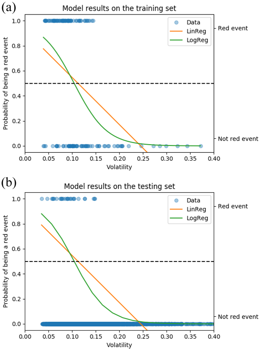At $σ = 15 %$ the logistic regression achieves 0.68 accuracy on the testing set and 0.64 accuracy on the training set when categorizing red events. This overall level of accuracy is expected as events to the left of the threshold contain both red and non-red events. While the threshold successfully contains the distribution of all the red events, it also captures a portion of the non-red events.

Figure 7.

Categorization of red versus non-red events on the basis of GARCH-modeled volatility. The green line plots predictive probabilities using logistic regression. The orange line plots predictive probabilities using linear regression. The top and bottom figures represent results for the training and testing sets, respectively.

Results from the logistic regression in Figure 7 suggest that in order to correct for the left-tail inducing behavior of the volatility scaling method, we need to take into account a volatility threshold. By introducing such a volatility floor, the volatility-scaling method can produce higher Sharpe Ratios for a given portfolio, even during periods of extreme low volatility.

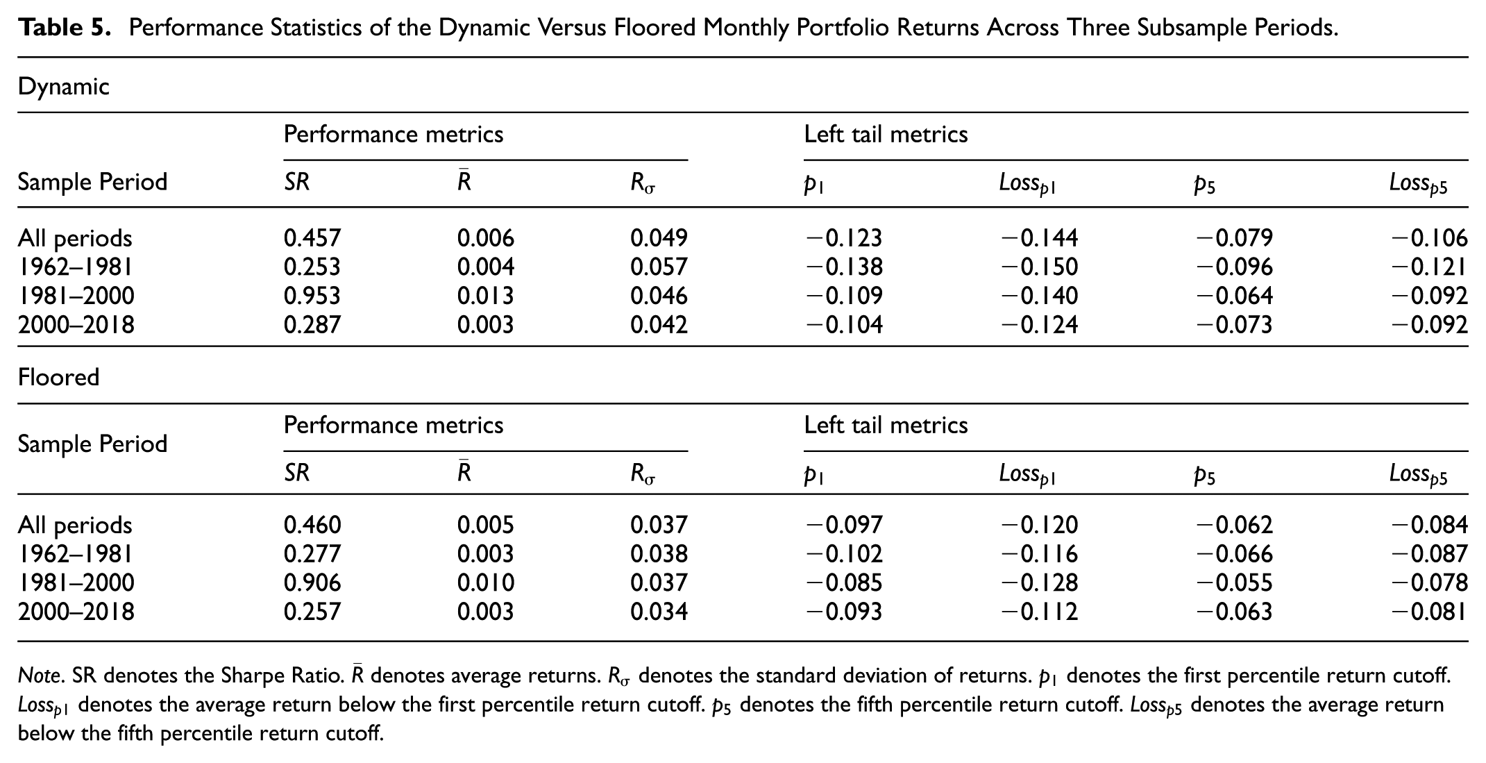
Recall that we select volatility floor d based on which σ gives the highest classification accuracy for left-tail events. Based the results from the logistic regression, we obtain the highest classification accuracy when we select $d = 0.15$ . For any choice of $d > 0.15$ , we observe an increase in false positive rates as events that are either in the left-tail of both the static and dynamic portfolio or events only in the left-tail of the static portfolio are also corrected. For any choice of $d < 0.15$ , we observe an increase in false negative rates.

Table 5 shows the summary statistics of the floored portfolio compared with the dynamic portfolio. As before, we include both results for the entire time period and for subsamples of our data. By implementing a volatility floor correction from 1962 to 2018, the Sharpe Ratio of the portfolio increases from 0.457 to 0.460. Thus, relative to its standard deviation, the floored portfolio delivers an excess of portfolio returns over the risk-free rate relative to the dynamic portfolio without a volatility floor correction. This improvement in Sharpe comes at the expense of delivering lower overall returns for the portfolio. This is a necessary trade-off between risk and returns for the portfolio holder and is not a surprising observation given the volatility floor is chosen to maximize the true positive rate of identifying a red event, at the expense of scaling down positions that do not fall in the volatility scaling induced left tail.

Table 5.

Performance Statistics of the Dynamic Versus Floored Monthly Portfolio Returns Across Three Subsample Periods.

Dynamic
	Performance metrics			Left tail metrics
Sample Period	SR	$\bar{R}$	$R_{σ}$	$p_{1}$	$Los s_{p 1}$	$p_{5}$	$Los s_{p 5}$
All periods	0.457	0.006	0.049	−0.123	−0.144	−0.079	−0.106
1962–1981	0.253	0.004	0.057	−0.138	−0.150	−0.096	−0.121
1981–2000	0.953	0.013	0.046	−0.109	−0.140	−0.064	−0.092
2000–2018	0.287	0.003	0.042	−0.104	−0.124	−0.073	−0.092
Floored
Sample Period	Performance metrics			Left tail metrics
	SR	$\bar{R}$	$R_{σ}$	$p_{1}$	$Los s_{p 1}$	$p_{5}$	$Los s_{p 5}$
All periods	0.460	0.005	0.037	−0.097	−0.120	−0.062	−0.084
1962–1981	0.277	0.003	0.038	−0.102	−0.116	−0.066	−0.087
1981–2000	0.906	0.010	0.037	−0.085	−0.128	−0.055	−0.078
2000–2018	0.257	0.003	0.034	−0.093	−0.112	−0.063	−0.081

Table 5 also shows that $p_{1}$ and $p_{5}$ over the full sample period are less negative for the floored portfolio than for the dynamic portfolio. More importantly, we report the expected loss of the portfolios below a certain percentile instead of a single cutoff point. The floored portfolio again demonstrates superior performance. The average of the lowest one percentile of returns is −0.120 for the floored portfolio, versus −0.144 for the dynamic portfolio, an improvement of 0.024 in log returns. Similarly, the average of the lowest five percentile of returns for the floored portfolio see an improvement of 0.022 in log returns over the dynamic portfolio alone.

We observe similar results for subsamples of the data. By incorporating the volatility floor correction, $Los s_{p_{1}}$ improved from 0.150 to −0.116 and $Los s_{p_{5}}$ improved from −0.121 to −0.087 over the time period 1962 to 1981. Compared with Table 2, these are precisely the metrics where the dynamic portfolio without a floor correction underperforms relative to the static portfolio. Comparison across the two tables suggest that the negative returns at the first and fifth percentiles for the volatility scaled portfolio are mitigated under a floor correction.

For ease of comparison, we also produce the distribution of returns for this particular subperiod in Figure 8. One way to interpret this distribution plot is that returns that would have been in the extreme left-tail of the dynamic portfolio are adjusted such that they are now closer to the center of the distribution. We note that similar adjustments to the return distribution are also seen for the subperiods 1981 to 2000 and 2000 to 2018.

Figure 8.

Distribution of returns of the floored versus the dynamic portfolio. Note the fatter left-tail of the orange distribution, which corresponds to the volatility scaled portfolio without a volatility floor correction.

Discussion and Implications

To assess the depth of the results presented in Section 4, we consider the performance of the volatility floor correction when returns are partitioned by market regimes as opposed to equal time periods. The intuition for this exercise is that if the volatility scaled portfolio performs worse during low volatility regimes compared with high volatility regimes, this provides further evidence for the need of a volatility floor correction.

Table 6 provides an additional robustness test by examining the performance of the dynamic volatility scaling strategy and the scaling strategy with a volatility floor correction under different market regimes. Reassuringly, we continue to see evidence in support of H2-H3. First, when comparing the left-tail of returns in the pre-Financial Crisis versus the post-Financial Crisis regime, we observe that despite not including market returns during the 2008 recession, the volatility scaled portfolio in the pre-crisis period results in more negative returns on average, conditional on returns being in the lowest first-percentile and fifth-percentile. For example, the pre-crisis volatility scaled portfolio delivers an average first-percentile of returns of −0.147 on the log scale, compared with returns of −0.129 on the log scale for the volatility scaled portfolio post-crisis. The comparison again provides evidence for H2 that negative returns can be introduced by the act of scaling itself.

Table 6.

Descriptive Statistics of Monthly Portfolio Returns Across Different Market Regimes.

Dynamic
	Performance metrics			Left tail metrics
Market Regime	SR	$\bar{R}$	$R_{σ}$	$p_{1}$	$Los s_{p 1}$	$p_{5}$	$Los s_{p 5}$
Pre-financial crisis	0.454	0.007	0.051	−0.126	−0.147	−0.082	−0.108
Post-financial crisis	0.476	0.005	0.043	−0.108	−0.129	−0.071	−0.093
Floored
	Performance metrics			Left tail metrics
Market Regime	SR	$\bar{R}$	$R_{σ}$	$p_{1}$	$Los s_{p 1}$	$p_{5}$	$Los s_{p 5}$
Pre-financial crisis	0.459	0.005	0.038	−0.098	−0.123	−0.062	−0.084
Post-financial crisis	0.464	0.005	0.034	−0.090	−0.108	−0.062	−0.080

Comparing both time periods to their counterparts in the bottom panel reproduce evidence consistent with H3, as was also shown in Table 5. In particular, we observe improvements across time periods and across all left-tail metrics when comparing the floored portfolio with the dynamic portfolio. For example, during the pre-crisis time period, the first percentile cutoff of the floored portfolio was −0.098, compared with the first percentile cutoff of the dynamic portfolio of −0.126. This suggests that implementing a correction in the form of a volatility floor correction introduced an improvement of 0.028 on the log scale. This is even larger in magnitude than any improvements in the subperiods in Table 5, suggesting that the ability of the floor correction in mitigating left-tail risks is not a function of the trading day breakpoints in Table 5. The improvement in performance is also seen in the post-crisis period. Again comparing the left-tail performance statistics of the bottom panel against the top panel, we observe that the floored portfolio exhibits improvement both on the cutoff and the average returns margin. For example, conditional on being in the lowest one percentile of returns, the portfolio with a volatility floor correction delivers expected returns of −0.108 on the log scale, compared with expected returns of −0.129 on the log scale for the scaled portfolio without such a correction, corresponding to any improvement of 0.021. Taken together, Table 6 provides additional robustness checks in favor of H2-H3.

It is not unreasonable to expect a risk-limiting method to also impact returns. For instance, if periods of low GARCH-estimated volatility coincide with periods of high returns, then imposing a volatility floor effectively constrains the extent to which the portfolio can be positively scaled. Consequently, the volatility floor places an upper-bound on portfolio returns. Given that this effect is already observed when comparing static versus dynamic portfolios, we assume that investors adopting the volatility-scaling strategy are comfortable with this trade-off. Here, we simply demonstrate the extent to which implementing a volatility floor impacts both tails, with the right tail corresponding to excess returns. To this end, Figure 9 plots of the returns generated by the dynamic portfolio over returns generated by the static portfolio.

Figure 9.

Comparison of daily returns generated by the dynamic versus floored portfolio. Events marked in red represent returns below the first percentile of the dynamic portfolio, but not the first percentile of the static portfolio. The top left, top right, bottom left, and bottom right figures plot the returns of the dynamic versus floored portfolio for 1962–2018, 1962–1981, 1981–2000, and 2000–2018, respectively.

Figure 9 shows the comparison of the static, dynamic, and floored portfolios. In each subpot, the x-axis and y-axis represent floored and dynamic returns, respectively, while red markers denote left-tail events caused by volatility scaling. If the volatility floor has no effect on the left-tail, we would expect to see red-events along the diagonal of the plot. If the volatility floor introduces additional left-tail events, we would expect to see red-events above the diagonal. Conversely, if the volatility floor mitigates the left-tail, we would expect to see red-events below the diagonal, a pattern observed in Figure 9. For example, consider the outlier red event shown in each subplot. Under volatility scaling with no volatility floor, this event generates −0.065 in log returns. With the volatility floor correction, the event generates −0.025 in log returns, corresponding to a 0.04 improvement in returns on the log scale.

Important for the discussion of trade-offs, however, we call attention to the right-tail displayed in the scatter plot, located in the top-right quadrant of each individual subplots. If volatility floor does not impact returns in the right-tail relative to the dynamic portfolio, we expect to see all points to the right of zero to be along the diagonal. If the volatility floor positively impacts red-tail returns, we expect to see some points to the right of zero to be below the diagonal. In this case, we see points to the right of zero above the diagonal, demonstrating that events that could have yielded superior returns under the dynamic portfolio are limited by the capping effect induced by the introduction of a volatility floor. In discussing the impact of the volatility floor on the right-tail, however, we point out that all events that delivered positive returns under the dynamic portfolio continue to deliver positive returns under the floored portfolio. To quantify the extent to which the right-tail returns are reduced, we report the equivalent statistics for the right-tail of returns for the dynamic versus the floored portfolio in Table 7.

Table 7.

Right-Tail Performance Statistics of the Dynamic Versus Floored Monthly Portfolio Returns Across Three Subsample Periods.

	Right tail metrics
	Dynamic				Floored
Sample Period	$p_{99}$	$Re t_{p 99}$	$p_{95}$	$Re t_{p 95}$	$p_{99}$	$Re t_{p 99}$	$p_{95}$	$Re t_{p 95}$
1962–1981	0.115	0.124	0.093	0.107	0.088	0.098	0.061	0.077
1981–2000	0.114	0.125	0.086	0.103	0.094	0.109	0.067	0.084
2000–2018	0.086	0.102	0.064	0.078	0.067	0.074	0.050	0.060

Note. $p_{99}$ denotes the 99th percentile return cutoff. $Re t_{p 99}$ denotes the average return above the 99th percentile return cutoff. $p_{95}$ denotes the 95th percentile return cutoff. $Re t_{p 95}$ denotes the average return above the 95th percentile return cutoff.

Table 7 reports the statistics $p_{99}$ , $p_{95}$ , $Re t_{p_{99}}$ , and $Re t_{p_{95}}$ for the volatility scaled portfolio without a floor correction and the volatility scaled portfolio with a floor correction. Of these, a more positive $p_{99}$ or $p_{95}$ corresponds to a more extreme right-tail. A more positive $Re t_{p_{99}}$ or $Re t_{p_{95}}$ corresponds to a higher expected return, conditional on being in the extreme right-tail as defined by percentile cutoffs. As shown visually in Figure 9, the trade-off of implementing the floor correction is the resulting capping of returns. For example, the 99th percentile of returns for the dynamic portfolio are 0.115, 0.114, and 0.086, respectively, across the three subperiods. The 99th percentile of returns for the floored portfolio are, respectively, 0.088, 0.094, and 0.067, corresponding to a decrease of 0.027, 0.020, and 0.019 on the log scale. This is comparable with the reduction in the left-tail as reported in Table 5. Recall that on average, the first percentile cutoff for returns is improved by 0.026 on the log scale, across all periods, when comparing the floored portfolio relative to the dynamic portfolio.

In order to consider the trade-offs from implementing the volatility floor correction, it is important to consider risk preferences of the investor employing these portfolio management strategies. From a theoretical perspective, assuming a concave utility function for portfolio managers, a larger left-tail induces greater disutility than a larger right-tail. Given that the expected reduction in the left-tail is comparable to the expected reduction in the right-tail, Table 5 and Table 7 provide evidence for a theoretical risk-averse investor to include a volatility floor correction when implementing the volatility scaling strategy.

Conclusion

Volatility scaling is a relatively new portfolio management method with growing academic attention. Prior empirical research suggests that such a method allows investors to adjust risk intertemporally and enhances the Sharpe ratio when applied to portfolios, particularly those composed of riskier assets. Focusing on the S&P index, this paper identifies a new drawback of this method and evaluates the effects of incorporating a volatility floor. Over the sample period 1962 to 2018, we show that implementing volatility scaling with a floor correction outperforms the volatility scaling method on left-tail risk metrics. This finding is robust to considering different subperiods and market regimes; the expected returns below the first percentile and fifth percentile are less negative for the volatility scaled portfolio with a floor correction than for the volatility scaled portfolio without such a correction.

The findings of this study have several empirical implications. First, one may wonder whether the volatility scaling method has any unintended consequences that are of interest to investors. We show that while volatility scaling improves the Sharpe Ratio relative to the traditional buy-and-hold portfolio, it also generates an unintended left-tail risk. Second, we provide a correction to the volatility scaling method that, to our knowledge, has not been previously introduced. The inclusion of this correction closely aligns with the objective of investors who use the volatility scaling method to manage left-tail risk. Importantly, results from this paper suggest that the inclusion of a volatility floor correction meaningfully reduces the left-tail generated by the scaling method.

Overall, this research adds to existing literature by bridging the gap between a new portfolio management method and practical risk management. The empirical results have direct implications for investor portfolio choice and asset allocation. While the method proposed in this paper sufficiently addresses the concern of left-tail risk induced by volatility scaling, it also introduces a trade-off between mitigating left-tail events and curbing returns. While such a trade-off is consistent with the standard risk-return framework and can be justified by the risk preferences of institutional investors, future research should focus on approaches which also minimize the reduction in right-tail outcomes.

Footnotes

ORCID iD

Qi Cui

Funding

The authors disclosed receipt of the following financial support for the research, authorship, and/or publication of this article.

Declaration of Conflicting Interests

The authors declared no potential conflicts of interest with respect to the research, authorship, and/or publication of this article.

Data Availability Statement

Data sharing not applicable to this article as no datasets were generated or analyzed during the current study.

References

Albeverio

Steblovskaya

Wallbaum

(2013). Investment instruments with volatility target mechanism. Quantitative Finance, 13(10), 1519–1528. https://doi.org/10.1080/14697688.2013.804943

Bai

Steblovskaya

Wallbaum

(2023), Improving retirement coverage durability with target volatility strategy for changing interest rate environment. Asia-Pacific Journal of Financial Studies, 52, 949–978. https://doi.org/10.1111/ajfs.12455

Barroso

Santa-Clara

(2015). Momentum has its moments. Journal of Financial Economics, 116, 111–120. https://doi.org/10.1016/j.jfineco.2014.11.010

Brennan

Schwartz

(1989). Portfolio insurance and financial market equilibrium. Journal of Business, 62(4), 455–472. https://doi.org/10.1086/296472

Chen

Worthington

(2022). Realised volatility and industry momentum returns. Humanities and Social Sciences Communications, 9, Article 287. https://doi.org/10.1057/s41599-022-01309-y

Cui

Zhao

Cui

(2023). Macroeconomic announcements: How announcements shape trading strategies. Sage Open, 13(4). https://doi.org/10.1177/21582440231218770

Dachraoui

(2018). On the optimally of target volatility strategies. Journal of Portfolio Management, 44(5), 58–67. https://doi.org/10.3905/jpm.2018.44.5.058

Daniel

Moskowitz

T. J.

(2016). Momentum crashes. Journal of Financial Economics, 122, 221–247. https://doi.org/10.1016/j.jfineco.2015.12.002

Di Persio

Garbelli

Wallbaum

(2021). Forward-looking volatility estimation for risk-managed investment strategies during the COVID-19 crisis. Risks, 9(2), 1–16. https://doi.org/10.3390/risks9020033

10.

Dopfel

Ramkumar

S. R.

(2013). Managed volatility strategies: Applications to investment policy. Journal of Portfolio Management, 40(1), 27–39. https://doi.org/10.3905/jpm.2013.40.1.027/

11.

Fleming

Kirby

Ostdiek

(2001). The economic value of volatility timing. Journal of Finance, 56(1), 329–352. https://doi.org/10.1111/0022-1082.00327

12.

Fleming

Kirby

Ostdiek

(2003). The economic value of volatility timing using ’realized’ volatility. Journal of Financial Economics, 67(3), 474–509. https://doi.org/10.1016/S0304-405X(02)00259-3

13.

Ghosh

(2010). Asset acquisition, diversification, and revision-theoretic exercises in portfolio theory. Quarterly Journal of Finance and Accounting, 49(1), 19–38. https://doi.org/10.2307/25747074

14.

Haddad

Kozak

Santosh

(2020). Factor timing. The Review of Financial Studies, 33(5), 1980–2018. https://doi.org/10.1093/rfs/hhaa017

15.

Hamill

Rattray

Hemert

O. V.

(2016). Trend following: Equity and bond crisis alpha. SSRN Electronic Journal. https://doi.org/10.2139/ssrn.2831926

16.

Harvey

C. R.

Hoyle, Korgaonkar

Rattray

Sargaison

Hemert

O. V.

(2018). The impact of volatility targeting. Journal of Portfolio Management, 45(1), 14–33. https://doi.org/10.3905/jpm.2018.45.1.014

17.

Hocquard

Papageorgiou

(2013). A constant-volatility framework for managing tail risk. The Journal of Portfolio Management, 39, 28–40. https://doi.org/10.3905/jpm.2013.39.2.028

18.

Hoyle

Shephard

(2018). Volatility scaling’s impact on the sharpe ratio. SSRN Electronic Journal. https://doi.org/10.2139/ssrn.3279787

19.

Just

Echaust

(2020). Stock market returns, volatility, correlation and liquidity during the COVID-19 crisis: Evidence from the Markov switching approach. Finance Research Letters, 37, Article 101775. https://doi.org/10.1016/j.frl.2020.101775

20.

Maillard

Roncalli

Teiletche

(2010). The properties of equally weighted risk contribution portfolios. Journal of Portfolio Management, 36(4), 60–70. https://doi.org/10.3905/jpm.2010.36.4.060

21.

Molyboga

(2020). Portfolio management of commodity trading advisors with volatility-targeting. Journal of Investment Strategies, 8(4), 1–20. https://doi.org/10.21314/JOIS.2020.116

22.

Moreira

Muir

(2017). Volatility managed portfolios. Journal of Finance, 72(4), 1611–1644. https://doi.org/10.1111/JOFI.12513

23.

Munir

Sukor

Shaharuddin

(2022). Adaptive market hypothesis and time-varying contrarian effect: Evidence from emerging stock markets of south asia. Sage Open, 12(1), 1–16. https://doi.org/10.1177/21582440211068490

24.

Naeem

M. A.

Yousaf

Karim

Yarovaya

Ali

(2023). Tail-event driven NETwork dependence in emerging markets. Emerging Markets Review, 55, Article 100971. https://doi.org/10.1016/j.ememar.2022.100971

25.

Perchet

de Carvalho

R. L.

Heckel

Moulin

(2015). Predicting the success of volatility targeting strategies: Application to equities and other asset classes. The Journal of Alternative Investments, 18(3), 21–38. https://doi.org/10.3905/jai.2016.18.3.021

26.

Poirier

(2021). Volatility targeting: The bridge between options-based and traditional defensive strategies. Journal of Portfolio Management, 47(6). https://doi.org/10.3905/jpm.2021.1.238

27.

Roncalli

Weisang

(2016). Risk parity portfolios with risk factors. Quantitative Finance, 16(3), 377–388. https://doi.org/10.1080/14697688.2015.1046907

28.

Shiraz

R. K.

Tavana

Fukuyama

(2020). A random-fuzzy portfolio selection DEA model using value-at-risk and conditional value-at-risk. Soft Computing, 24, 17167–17186. https://doi.org/10.1007/s00500-020-05010-7

29.

Stewart

Piros

Heisler

(2019). Portfolio management: Theory and practice (2nd ed.). McGraw-Hill.

30.

Tavana

Shiraz

R. K.

Di Caprio

(2019). A chance-constrained portfolio selection model with random-rough variables. Neural Computing & Applications, 31(2), 931–945. https://doi.org/10.1007/s00521-017-3014-8

Mitigating Left-tail Risk in Volatility Scaling: Introducing a Volatility Floor Correction

Abstract

Plain Language Summary

Keywords

Introduction

Literature Review

Volatility Scaling as a Portfolio Management Strategy

Evaluation of Volatility Scaling in Practice

Research Gaps and Hypothesis Formation

Data and Methods

Static Buy-and-Hold Portfolio

Dynamic Volatility Scaled Portfolio

Volatility Scaled Portfolio with a Floor Correction

Results

Returns Comparison Analysis

Subsample Analysis

Performance of the Volatility Floor Correction

Discussion and Implications

Conclusion

Footnotes

ORCID iD

Funding

Declaration of Conflicting Interests

Data Availability Statement

References