Sage Journals: Discover world-class research

Abstract

As concerns around climate change and global warming intensify, extreme weather events such as heavy rain, blizzards, and smog-induced haze have greatly impacted the commuting travel mode selection of urban residents. Such behavioral shifts have in turn led to changes of the carbon emissions generated from these residents. This paper constructs a “extreme weather (W)–travel behavior (B)–carbon emissions (C)” research framework. Using a multiple logistic regression model, the transportation mode shift model, and the econometric model of urban resident’s travel behavior under the influence of extreme weather conditions were constructed. The marginal effects of weather on residents’ commuter behavior, through the use of transportation type and distance of travel were also obtained. The study found that the overall carbon dioxide emission levels of daily commuting has gradually decreased due to the influence of extreme weather. However, as some travelers still adopted high-emission commuting modes through the use of taxis or ride-sharing services, there was still a slight increase in CCDE levels in certain extreme weather contexts. In particular, when haze was prevalent, vehicle restriction policies only reduced CCDE by 2.18%, while the remaining 77.83% of total CCDE remaining unchanged. This research provides a key reference point for governmental departments in urban transportation management and environmental protection to formulate policies.

Keywords

extreme weather commuting travel mode selection carbon dioxide emissions marginal effect vulnerability

Introduction

As climate change concerns deepen, improving our understanding of urban transportation carbon emissions has become an increasingly important area of academic inquiry (Brand & Preston, 2010; Sikder et al., 2022). As part of this, has been an exploration of the changes of carbon emission structure and clarifying the key mechanisms that have been at the forefront of these developments. Current research into the evolution of carbon emissions involving residential commuting can be divided into two fields of analysis. The first is to analyze, from a planning perspective, the quantificational impact that urban spatial environmental characteristic such as land use, urban scale, and urban form have on urban commuting and its associated carbon emissions (Abenoza et al., 2019; Cervero, 1996; P. Chen et al., 2012; Yang et al., 2020; Yi et al., 2021). The second is to analyze, from an individual behavior perspective, the impact that family-based socioeconomic characteristics, such as the individual’s income, age composition, family location and other relevant attributes have on urban commuting and its associated carbon emissions (Brand et al., 2013; Chai et al., 2012; Gong et al., 2013; C. Q. Liu et al., 2018). Urban transportation carbon emissions are complex involving multiple levels of economic, social, and environmental factors (Wang, Wood, Geng, Wang, & Long, 2020; Wang, Wood, Geng, Wang, Qiao, et al., 2020; Wang, Zhao, et al., 2020). Recently, global warming and climate change concerns have been at the forefront of much research, particularly in regards to the commuting travel mode selection of urban residents (AI Duhayyim et al., 2022; Dijst et al., 2013; Koetse & Rietveld, 2009). For example, excessive precipitation in summer and large-scale snowfall in winter affects urban road traffic conditions and thus reduces road capacity, forcing travelers to adopt other modes of transportation. On the other hand, air pollution levels in many cities around the world is of growing concern. In order to reduce air pollution, the government can adopt policies that restrict the number of vehicles that are driven on the road (Böcker et al., 2013; Chowdhury et al., 2017; Z. Y. Liu, Li, et al., 2017). Such measures can have quite profound impacts on those who use cars for daily commuting purposes. Therefore, these road users may need to use public forms of transportation, such as subways, buses, etc. Existing research shows that weather and climatic conditions have a significant impact on urban residents’ traveling behavior (Ferri-Garcia et al., 2020; Koetse & Rietveld, 2009). However, most research has focused on the negative impact that extreme weather has had on regional transportation systems, with little attention given to how extreme weather events impact residential travel behavior (Fu et al., 2014; Zanni & Ryley, 2015). As climate change and global warming intensifies, the impact that extreme weather events can have on travel behavior will become more pronounced, which will further implications for related carbon emission levels.

Although people are increasingly aware of the impact that extreme weather can have on residential travel behavior, these insights cannot be directly used as a means of analyzing the quantitative effects of weather changes on urban commuters’ carbon dioxide emissions (CCDE). Changes in weather patterns and global climatic conditions may lead to the increases or decreases in distances people travel, however, these effects may be offset by changes in the emission levels related to the new modes of transportation that may be used. For example, heavy rainfall can tend to reduce travel distances and increase the likelihood of travel by car (Koetse & Rietveld, 2009). Therefore, the amount of carbon dioxide emissions generated by individual commuters does not necessarily increase. Actually, the mechanism from which urban commuter’s carbon dioxide emissions are affected by weather changes is highly complex. The changing characteristics of carbon dioxide emissions from urban commuters will be a key feature of future climate change scenarios and an important field of focus for researchers and policymakers. Some scholars have long been concerned about the impact of weather change on commuter travel behavior and has conducted a series of studies on this issue (de Kuijf et al., 2021; Lin et al., 2020; C. Q. Liu et al., 2015a, 2015b, 2015c). An econometric model was established by some scholars to firstly describe the marginal impacts of weather conditions on commuter travel behavior, and then secondly calculating the relevant changes in commuter-based carbon dioxide emissions using five climatic scenarios (C. Q. Liu et al., 2015a). Since individual activity-travel patterns change under different weather conditions, some scholars also have studied the changes in carbon dioxide emissions with changes in weather conditions. Existing studies have shown that both seasonal and traffic conditions are responsible for significant changes in CO₂ emissions (Romano et al., 2021), and that changes in CO₂ emissions under climate warming and extreme temperature scenarios tend to be larger than the sum of changes in CO₂ emissions under each scenario (C. Q. Liu et al., 2016). In summary, current research has mainly focused on the impact of climate change on urban commuter travel behaviors, while analysis of the effects of travel behavior change on urban commuter carbon dioxide emissions is still very much an emerging field of scholastic inquiry.

Urban commuter transportation refers to a person’s daily travel to and from work. Especially in China, urbanization has spawned a number of large cities with a population of more than 10 million (e.g., Emerging national central cities in China-Xi’an city). This means that nearly half of the population will choose different means of transportation to travel during the morning and evening traffic peak time in these cities. Therefore, the impact of extreme weather on the resilience of urban traffic continues to receive attention. As such, the process includes very rigid time constraints, and 58.4% of China’s total urban transportation demand is residential commuter travel (Ben et al., 2016; C. Q. Liu, Shi, et al., 2017). In recent years, extreme weather events such as rainstorms, snowstorms, or haze have continued to have a greater influence on the travel behavior of Chinese urban residents. In particular, restrictions on vehicle use bought about by winter haze have greatly influenced the travel behaviors of urban residents, forcing them to adopt other forms of transportation in order to live their daily lives. This situation is more obvious in western cities of China, and shifts in how people travel is undoubtedly changing carbon emission levels. In order to explore these carbon dioxide emission changes, C. Q. Liu et al. (2016) derived the marginal effects of weather variables on each travel behavior variable and used them to calculate travel behavior changes under new weather scenarios. These travel behavior changes, along with changes in emission factors, were then used to derive changes in CO₂ emissions. Inspired by this research, we recommend using a framework that employs “extreme weather (W)–travel behavior (B)–carbon emissions (C).” The key unique aspects of this research are as follows. (1) We propose the use adoption of a “extreme weather (W)–travel behavior (B)–carbon emissions (C)” framework. Using a multiple logistic regression model, the transportation mode shift model, and the econometric model of urban resident’s travel behavior under the influence of extreme weather conditions were constructed. (2) The marginal effects of weather on residents’ commuter behavior, through the use of transportation type and distance of travel were also obtained. (3) This effect was in turn used to calculate the relevant commuter travel carbon dioxide emissions and the extent to which travel behavior change had impacted these levels, Considering that the small impact of light rain, light snow, high temperatures, and other weather conditions on urban residents’ commuting. It should be noted that this study only analyzed the impact of extreme weather events such as the rainstorm, snowstorm, and haze.

The rest of this study is arranged as follows. Section 2 proposes the “W–B–C” analysis framework and describes the transition process of extreme weather events on commuter travel behavior and carbon dioxide emissions. Section 3 constructs the transportation mode shift model, the econometric model of the impact of extreme weather on travel behavior, and the commuting carbon emission calculation model. Section 4 analyzes the impact that various extreme weather events have on changes in commuter carbon dioxide emissions in Xi’an, China. Finally, some concluding remarks and related recommendations are provided at the end of the study.

The Analysis Framework

According to our analysis above, extreme weather events such as the rainstorms, snowstorms, and haze have an impact on the travel behaviors of urban commuters. These weather events will, in turn, affect the level of carbon dioxide emissions generated by these urban commuters due to differences in the types of transportation modes that these residents may adopt. On this basis, our study proposes a “Weather–Behavior–Carbon” (W–B–C) analysis framework to describe the impact and changes that extreme weather events have on urban commuter carbon emissions (see Figure 1).

Figure 1.

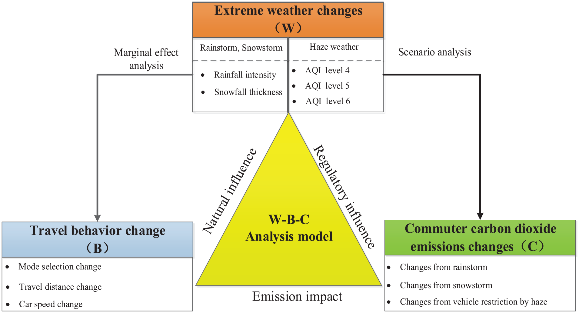
W-B-C analysis framework.

The “W” part of Figure 1, examines extreme weather events, which can be divided into two categories. The first includes rainstorms and snowstorms, while the second includes smog-related haze. These two types of extreme weather influence residents’ travel behavior in different ways. Rainstorm and snowstorm generally lead to a deterioration in natural weather conditions, and as such they reduce the capacity of local road transportation networks. Although hazy weather conditions may not directly lead to urban transportation systems becoming paralyzed, the implementation of urban traffic pollution reduction policies have ensured that when the air pollution reaches a certain level, governments have utilized vehicle restriction strategies, including the One-Day-Per-Week (ODPW) and Odd-And-Even (OAE), which have forced residents to change the way they commute (Z. Y. Liu, Li, et al., 2017). The ODPW policy forces private cars off the road 1 day per week (20% of vehicles are restricted/day), while the OAE policy allows private cars to be used on the road according to the odd/even numbers shown on their license plates (50% of vehicles are restricted/day). The restrictive nature of these policies has meant that many commuters have abandoned the use of private cars by deciding to use greener modes of transportation such as city buses, the subway, riding a bike, or even walking. In Section “B” section, as a consequence of extreme rain and/or snowstorms, traffic capacity on the roads is reduced, or in the case of haze, vehicle numbers are restricted on urban roads. These situations may change the commuter travel behavior of urban residents (such as the mode of transportation they use or the distance they travel, etc.). Using Xi’an, China, as an example, the city utilizes a dynamic vehicle restriction policy during period of severe air pollution. In this instance, when the air quality index (AQI) reaches level 4 or level 5, the ODPW policy is immediately triggered. Moreover, if the problem reaches level 6, the local Government implements its OAE policy, as shown in Table 1. In “C” section, as a result of changes in urban commuter behaviors due to various extreme weather events, the factors used to measure carbon dioxide levels for urban commuters will also change, thereby affecting total emissions as well (see Figure 2).

Table 1.

Xi’an Vehicle Restriction Policy During Period of Heavy Air Pollution.

AQI	AQI level	Vehicle restriction policy	Policy impact
0–50	Level 1 (excellent)	No vehicle restriction	None
51–100	Level 2 (good)	No vehicle restriction	None
101–150	Level 3 (light pollution)	No vehicle restriction	None
151–200	Level 4 (moderate pollution)	One-Day-Per-Week	20% of vehicles are restricted per day
201–300	Level 5 (severe pollution)	One-Day-Per-Week	20% of vehicles are restricted per day
301+	Level 6 (serious pollution)	Odd-and-even	50% of vehicles are restricted per day

Figure 2.

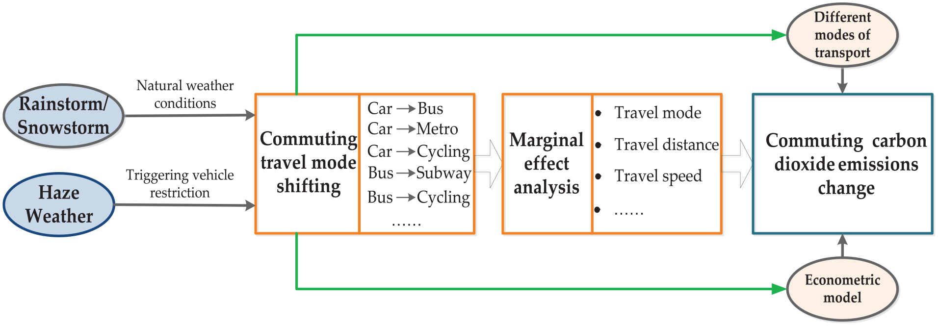
Change analysis framework for commuter carbon dioxide emissions.

Research Model

Transportation Mode Shift Model

Under the influence of extreme weather events, such as rainstorms, snowstorms and haze, the urban commuters’ transportation mode will shift. This shift in behavior to adopt alternative forms of transportation, can be described using a shift matrix, which is around the probability of a shift occurring, which is called the transportation mode shift matrix (S). Sⁱ describes the probability of a shift occurring in the commuters’ chosen form of transportation mode, including the use of private cars, buses, subways, and bicycles (walking), as shown in Formula (1).

\begin{array}{l} c a r b u s m e t r o c y c l i n g \\ S^{i} = \begin{matrix} c a r \\ b u s \\ m e t r o \\ c y c l i n g \end{matrix} {[\begin{matrix} S_{11}^{i} \\ S_{21}^{i} \\ \dots \\ S_{m 1}^{i} \end{matrix} \begin{matrix} S_{12}^{i} \\ S_{22}^{i} \\ \dots \\ S_{m 2}^{i} \end{matrix} \begin{matrix} \dots \\ \dots \\ \dots \\ \dots \end{matrix} \begin{matrix} S_{1 m}^{i} \\ S_{2 m}^{i} \\ \dots \\ S_{m m}^{i} \end{matrix}]}_{m \times m} \end{array}

(1)

where Sⁱ is the transportation mode shift matrix of commuter i, and sⁱ_jk is the shift probability of commuter i in n transportation mode. The solution of the shift probability sⁱ_jk can be performed using a multiple logistic regression method. Logistic regression is currently the most widely used modeling method for dealing with causal variables such as probabilities or proportional problems (W. Chen et al., 2018; Seo et al., 2018; Simone et al., 2018; Wu et al., 2018; Zhao & Chen, 2016). Therefore, based on the RP + SP tracking survey of certain commuters, this study uses a multiple logistic regression method to construct a urban commuters transportation mode shift model, given an extreme weather event, and then analyze its statistically significant impact factor.

Multiple logistic regression is an extension of the binomial logistic regression model. It is divided into an ordered multiple logistic model and a disordered multiple logistic model. Disordered multiple logistic regression models are used in this study because there is no incremental or decreasing order relationship between the selected proportions of transportation modes studied. Assuming that the dependent variable has m categories, the conditional probability of each category of the dependent variable is

P_{k}^{i} = P (y = k | x_{i j}) = \frac{e^{α_{k} + \sum_{i = 1}^{n} β_{i k} x_{i}}}{\sum_{k \in C_{k}} e^{α_{k} + \sum_{i = 1}^{n} β_{i k} x_{i}}}

(2)

where P_kⁱ is the probability that the commuter i chooses the transportation mode k; y is the dependent variable, which indicates the choice of transportation used by the commuter; C_k is the variable selection set; x_i is the independent variable (i = 1, 2,. . ., n, j = 1, 2, . . .,l), j is the dummy variable label, and α_k and β_ik are the parameters to be calibrated. Multiple logistic regression is modeled by fitting a generalized Logit model. First, we select a certain category, such as cars as a reference class. For example, if class 1 is used as the reference class, α_k and β_ik are equal to 0, and the conditional probabilities of the reference class and other categories are

P_{1}^{i} = P (y = 1 | x_{i j}) = \frac{1}{\sum_{k \in C_{k}} e^{α_{k} + \sum_{i = 1}^{n} β_{i k} x_{i}}},

(3)

P_{q}^{i} = P (y = q | x_{i j}) = \frac{e^{α_{q} + \sum_{i = 1}^{n} β_{i q} x_{i}}}{\sum_{q \in C_{q}} e^{α_{q} + \sum_{i = 1}^{n} β_{i q} x_{i}}}

(4)

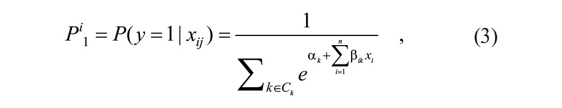
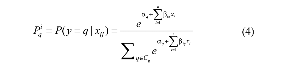
Then, each category is compared with the reference class to obtain (m − 1) generalized logit models. For example, the research object in this study is the choice of transportation modes, given specific extreme weather events. The choice of transportation mode is cars, buses, subways, and bicycles (walking), and they are expressed as P₁ⁱ, P₂ⁱ, P₃ⁱ, P₄ⁱ, respectively. If cars are used as a reference class, we are able to obtain the following general logit model:

s_{j k}^{i} = \ln (\frac{p_{j}^{i}}{p_{k}^{j}}) = α_{j} + \sum_{i = 1}^{n} β_{i j} x_{i}

(5)

s_{12}^{i} = \ln (\frac{p_{2}^{i}}{p_{1}^{i}}) = α_{2} + \sum_{i = 1}^{n} β_{i 2} x_{i}

(6)

s_{13}^{i} = \ln (\frac{p_{3}^{i}}{p_{1}^{i}}) = α_{3} + \sum_{i = 1}^{n} β_{i 3} x_{i}

(7)

s_{14}^{i} = \ln (\frac{p_{4}^{i}}{p_{1}^{i}}) = α_{3} + \sum_{i = 1}^{n} β_{i 3} x_{i}

(8)

s . t . p_{1}^{i} + p_{2}^{i} + p_{3}^{i} + p_{4}^{i} = 1

where $p_{1}^{i} p_{2}^{i} p_{3}^{i} p_{4}^{i}$ are the probability of choosing a car, bus, subway, bicycle (walking) for commuter i under a respective extreme weather event; x_i is the indicator (including extreme weather variables) that affects urban commuter travel choices; α_k and β_ik are the regression intercept and regression coefficients of the model, corresponding to different intercepts and coefficients for each generalized logit model.

Marginal Effect of Extreme Weather on Residents’ Commuting Travel Behaviors

In Section 3.1, the multiple logistic regression method is used to measure the changes of urban commuter behavior caused by the effects of extreme weather x_i. In order to further express the changes in commuter transportation behavior caused by a change in a unit weather variable, this study proposes the Marginal Effect of urban commuter behavior. Taking a shift in the mode of commuter transportation as an example, the marginal effect of extreme weather on urban commuter behavior is illustrated (travel distance and driving speed are the same) in Formula (9).

M E_{k}^{i} = \frac{\partial P_{k}^{i}}{\partial x_{i}} = \lim_{Δ x_{i} \to 0} \frac{P_{k}^{i} (x_{i} + Δ x_{i})}{Δ x_{i}} = \frac{\int_{- \infty}^{\infty} \frac{e^{α_{q} + \sum_{i = 1}^{n} β_{i q} (x_{i} + Δ x_{i})}}{\sum_{q \in C_{q}} e^{α_{q} + \sum_{i = 1}^{n} β_{i q} (x_{i} + Δ x_{i})}} f (μ_{i}) d μ_{i} - \int_{- \infty}^{\infty} \frac{e^{α_{q} + \sum_{i = 1}^{n} β_{i q} x_{i}}}{\sum_{q \in C_{q}} e^{α_{q} + \sum_{i = 1}^{n} β_{i q} x_{i}}} f (μ_{i}) d μ_{i}}{Δ x_{i}}

(9)

where Δx_i represents a small change in the given weather variable x_i. In this study, Δx_i takes 1% of the mean of x_i values of all samples. $M E_{k}^{i}$ is the marginal effect of extreme weather on urban commuter travel behavior, characterizing the change in the probability of a dependent variable due to a unit change in a given weather variable. For the purpose of this study, the integral in Formula (9) can be solved using MATLAB simulation technology.

Changes in Carbon Dioxide Emissions From Commuter Transportation, Under an Extreme Weather Scenario

Given an extreme weather context, although the marginal effect provides an explanation of the changes in carbon dioxide emissions that occur in an urban commuter transportation environment, the actual quantitative characteristics of the changes remain unclear. The marginal effect of extreme weather variables on urban commuter carbon dioxide emissions can be derived from an econometric model. In order to obtain the change in carbon dioxide emissions from this commuter group, the variable change in commuter behavior is obtained through Section 3.2

The amount of carbon dioxide emitted by urban commuters depends on a range of emission factors and the distance of travel involved. The most effective means of estimating the carbon dioxide emission from urban commuters, is to use the unit travel volume of the different transportation modes to calculate the total energy consumption and its subsequent carbon dioxide emissions (Feng et al., 2016; Simone et al., 2018). Based on a combination of the current literature and the actual characteristics of the Xi’an urban commuters travel activities, as well as the direct energy consumption levels of the vehicles used, we intend to adopt the “Carbon emission intensity table for Chinese mass transit” as issued by the Lvyuan Group. We also refer to the EU 2006 TREMOVE2.4 manual to ascertain the carbon dioxide emission intensity indicators for the various transportation modes utilized in our study (X. Y. Zhang et al., 2014; (Table 2).

Table 2.

Carbon Dioxide Emission Intensity For the Different Transportation Modes.

Number	Transportation	Carbon dioxide emission intensity (g/person·km)	Intensity grading
1.	Private car	135	High
2.	Bus	37	Medium
3.	Subway	9.10	Low
4.	Bicycle/walking	0	Zero

Urban commuters’ carbon dioxide emissions (CCDE) can be calculated by using the product sum for the carbon emission factor and distance traveled at each stage of the trip (X. Huang et al., 2015; J. C. Huang, & Lin, 2017; Sheyda et al., 2012), as shown in Formula (10).

C C D E_{i} = \sum_{j = 1}^{n} d_{j} \times e_{j}

(10)

where CCDE_i is the total level of carbon dioxide emissions generated through the daily travel by commuter i (g); j is the transportation mode used; d_j is the total distance traveled by the transportation mode j (km); e_j is the carbon dioxide emission intensity per unit of distance traveled using transportation mode j (g/person·km). Changes in carbon dioxide emissions due to the adoption of different transportation modes, under extreme weather conditions, can be measured using Formula (11).

Δ C C D E_{i} = \sum_{j = 1}^{n} d_{j} \times e_{j} - \sum_{j^{'} = 1}^{n} d_{j^{'}} \times e_{j^{'}}

(11)

where the ΔCCDE_i represent the amount of change in carbon dioxide emissions generated by commuter i before and after the change in transportation mode due to extreme weather (g); j′ is the new transportation mode; d_j_′, e_j_′ is the distance traveled and the carbon dioxide carbon emission factor of the mode j′, respectively.

Variable Selection

Shifts in the urban commuters’ mode of transportation as well as changes in carbon dioxide emission due to extreme weather events are now discussed. There are four modes of transportation type: car, bus, subway, and bicycle (walking). Based on the above analysis, we build a transportation mode shift model based on multiple logistic regressions to analyze the changes in commuter travel behavior and carbon dioxide emissions under extreme weather conditions (F. Zhang et al., 2018). Therefore, commuter transportation mode shift and carbon dioxide emissions are used as dependent variables, and the explanatory variables are divided into individual demographic characteristics (including gender, age, education level, occupation, income, family structure, and private car ownership), commuter transportation information variables (including daily round trips, weekly commuting days, and transportation mode), and weather attribute variables (including rainstorms, snowstorms, and haze). The variable settings are shown in Table 3.

Table 3.

Group and Explanation of Independent Variables.

Variable classification	Variable name	Sign	Variable description
Personal demographics Characteristic	Gender	X1	1. Male
	Gender	X1	2. Female
	Age	X2	1. 20 years old and below
			2. 21–40 years old
			3. 41–60 years old
			4. 60 years old older
	Occupation	X3	1. State organs, party organizations, enterprises, and institutions
			2. Professional technology and cultural and educational personnel
			3. Private owners
			4. Business and service personnel
	Education	X4	1. High school and below
			2. College or technical school
			3. Undergraduate
			4. Master degree and above
	Family structure	X5	1. Single
			2. A couple
			3. A couple and one child
			4. A couple and more than two children
			5. Other
	Income	X6	1. 3,000 yuan or less
			2. 3,001–5,000 yuan
			3. 5,001–8,000 yuan
			4. 8,001–15,000 yuan
			5. 15,001–20,000 yuan
	Private car	X7	1. No car
			2. One car
			3. More than two cars
Commuting information variable	Daily round trips	X8
	Weekly commute days	X9
	Transportation mode	X10	1. Private car
			2. Bus
			3. Subway
			4. Walking/bicycle
			5. Taxi
Weather attribute	Rainfall	X11	1. 5.0–16.9 mm/24 hours (light rain–moderate rain)
			2. 17.0–37.9 mm/24 hours (moderate rain–heavy rain)
			3. >50 mm/24 hours (above heavy rain)
	Snowfall	X12	1. 2.5–4.9 mm/24 hours (medium snow)
			2. 3.8–7.4 mm/24 hours (medium to heavy snow)
			3. 5.0–9.9 mm/24 hours (heavy snow)
			4. 7.5–14.9 mm/24 hours (heavy snow to blizzard)
	Air quality	X13	1. Excellent
			2. Mild pollution
			3. Moderate pollution
			4. Heavy pollution
			5. Serious pollution

Research Area and Data Sources

Xi’an is one of the nine largest cities, emerging national central cities in China. It is located in the central part of China, where it enjoys a warm temperate semi-humid continental monsoon climate. However, in recent years, extreme weather events, such as the rainstorms, snowstorms, and haze have occurred frequently in Xi’an, with 2016 and 2017 being particularly severe. During this time, heavy rainfall of more than 16.9 mm falling over a 24-hour period occurred some 20 times in summer. While in winter heavy snow falls were recorded in which 7.4 mm of snow fell over a 24-hour period on 10 occasions. At the same time, the city also experienced concerning levels of air pollution, with 35% of this period classified as having moderate levels of haze. In response to this, the Government introduced the ODPW and OAE vehicle restriction policies. These extreme weather events have greatly affected the ways in which the city’s residents commute, and as a consequence the levels of carbon dioxide emissions generated by its residents. Given this context, the city of Xi’an represents an ideal place to investigate these impacts.

Furthermore, as part of our analysis, we examine the effects of extreme weather events at different locations across Xi’an. These areas include the central and marginal areas (Lianhu District, Yanta District, Weiyang District, Chang’an District, and Lintong District), which can represent different urban spatial structures. Moreover, the residents’ transportation preferences across the different regions also have their own characteristics (Lin et al., 2020). Taking into account the time when extreme weather is prone to occur, the investigation was carried out from November 15, 2016 to March 15, 2017 (city heating), from June 1, 2017 to August 30, 2017 (summer), and from December 1, 2016 to February 28, 2017 (winter). The stratified sampling method was used to track the travel activities of 130 residents in the above five districts according to the demographics of the community. From this assessment, our study obtained 5,848 pieces of travel activity information (see Table 4). The scope of the survey is shown in Figure 3. In addition to the tracking data that was collected, we also obtained weather data from the following official websites: the “National Meteorological Information Center (2021),” the “Shaanxi Provincial Meteorological Bureau (2021),” and the “Xi’an real-time Air Quality Index (2021).”

Table 4.

The Stratified Sampling Result.

Commuter travel location	Number of commuters	Number of commuting activities	Proportion (%)
Lianhu district	28	1,145	19.6
Yanta district	27	1,268	21.7
Weiyang district	25	1,331	22.8
Chang’an district	23	1,123	19.2
Lintong district	27	981	16.7

Figure 3.

Overview of the study area.

Empirical Research

Analysis of the Impact of Extreme Weather on Residents’ Commuting

By tracking the individual commuter travel data, we are able to develop the commuter transportation shift model. The likelihood ratio test is performed to ascertain whether all of the partial regression coefficients of the independent variable are zero in the model (see Table 5). The results show the following:

(1) Under the influence of rainstorm, the (−2) times log-likelihood value is 2,653.39, when the independent variables are not introduced into the transportation mode shift model, while it reduced to 2,612.32 after introducing these variables. The difference between the two situations is equal to 41.07, and the degree of freedom is 13 and p < .001, indicating that the partial regression coefficient of at least one independent variable is not zero, which illustrates the robust nature of the model.

(2) Under the influence of snowstorm, the (−2) times log-likelihood value is 2,574.46 when the independent variables are not introduced into the commuter transportation mode shift model, while it reduced to 2,524.72 after introducing these variables. The difference between the two situations is equal to 43.74, and the degree of freedom is 13 and p < .001, indicating that the partial regression coefficient of at least one independent variable is not zero, again highlighting appropriateness of the model.

(3) Under the influence of haze, the (−2) times log-likelihood value is 2,496.53 when the independent variables are not introduced in the commuter transportation mode shift model, while it reduced to 2,432.31 after introducing these variables. The difference between the two situations is equal to 64.22, and the degree of freedom is 13 and p < .001, indicating that the partial regression coefficient of at least one independent variable is not zero, indicating that the model is meaningful. The rest are similar. It can be seen that the transportation mode shift model likelihood ratio test results, for urban commuters traveling in heavy rainstorms, snowstorms, and hazy weather conditions are shown in Table 5. Variables such as occupation, income, private car, commuter transportation mode, rainstorm, snowstorm, and hazy weather have significant effects on the shift model. By tracking the survey data, Table 6 provides the parameter calibration results of the commuter transportation mode shift model under the influence of rainstorms, snowstorms, and haze (B is the partial regression coefficient).

Table 5.

Likelihood Ratio Test Result.

Variable effect	Model fitting criteria			Likelihood ratio test
	(−2) Times log-likelihood value of the simplified model			χ²				Significant level
	Rainstorm	Snowstorm	Haze	Rainstorm	Snowstorm	Haze	df	Rainstorm	Snowstorm	Haze
Intercept	2,565.73	2,432.92	2,398.27	0	0	0	—	—	—	—
X3	2,612.32	2,524.72	2,432.31	24.325	22.458	21.318	1	.002	.000	.001
X4	2,554.78	2,476.13	2,329.34	23.321	22.237	21.497	1	.000	.003	.003
X6	2,542.67	2,454.71	2,445.39	25.672	23.568	24.372	0	.001	.000	.002
X7	2,513.35	2,418.38	2,408.24	23.371	21.487	20.257	1	.002	.001	.003
X10	2,556.78	2,431.45	2,467.87	26.315	23.479	22.871	1	.001	.001	.000
X11	2,546.14	2,498.24	2,498.25	25.476	24.248	24.798	1	.003	.003	.000
X12	2,346.90	2,239.64	2,317.49	24.128	22.271	21.477	1	.001	.001	.000
X13	2,489.26	2,356.38	2,276.15	23.174	21.983	22.157	1	.002	.002	.000

Table 6.

Parameters Calibration Results of Commuting Mode Shift Model Under the Extreme Weather.

Rainstorm							Snowstorm						Haze
Variables		B	SE	Wald	df	Significant level	Variable	B	SE	Wald	df	Significant level	Variable	B	SE	Wald	df	Significant level
Car→bus	X3	0.34	0.19	10.23	1	.002	X3	0.67	0.34	7.32	1	.012	X3	0.75	0.32	4.31	1	.024
	X4	0.22	0.12	4.59	1	.421	X4	0.35	0.27	9.45	1	.532	X4	0.46	0.23	5.49	1	.031
	X6	−0.13	0.43	2.46	0	.036	X6	0.46	0.23	3.74	0	.023	X6	0.58	0.28	2.62	0	.012
	X7	0.58	0.36	5.67	1	.012	X7	0.47	0.26	6.69	1	.023	X7	−0.68	0.34	5.62	1	.023
	X10	0.79	0.44	6.23	1	.059	X10	0.53	0.21	4.24	1	.053	X10	1.57	0.76	3.21	1	.042
	X11	0.94	0.57	2.70	1	.029	X12	0.79	0.47	3.52	1	.018	X13	0.36	0.17	2.36	1	.027
Car→subway	X3	0.56	0.28	7.29	1	.017	X3	0.46	0.26	1.32	1	.034	X3	0.25	0.16	1.74	1	.012
	X4	0.74	0.38	3.57	1	.259	X4	0.57	0.39	2.58	1	.154	X4	0.37	0.19	2.65	1	.145
	X6	−0.36	0.57	3.94	0	.027	X6	0.39	0.17	2.45	0	.037	X6	0.47	0.29	2.54	0	.021
	X7	0.76	0.47	4.32	1	.010	X7	0.86	0.49	3.31	1	.019	X7	0.54	0.29	4.15	1	.029
	X10	0.68	0.34	8.26	1	.063	X10	0.32	0.14	5.23	1	.032	X10	−0.98	0.44	5.63	1	.031
	X11	0.54	0.27	3.78	1	.017	X12	0.67	0.42	4.79	1	.026	X13	0.77	0.36	2.72	1	.028
Car→walking	X3	0.43	0.22	4.28	1	.026	X3	0.21	0.14	3.12	1	.014	X3	−0.65	0.34	2.62	1	.024
	X4	0.54	0.28	2.55	1	.235	X4	0.64	0.32	2.32	1	.312	X4	0.57	0.31	3.41	1	.334
	X6	−0.39	0.39	2.85	0	.019	X6	0.57	0.42	3.89	0	.021	X6	−0.79	0.32	2.82	0	.015
	X7	0.58	0.27	3.36	1	.014	X7	0.78	0.29	2.45	1	.023	X7	0.45	0.21	2.31	1	.027
	X10	0.59	0.24	7.18	1	.042	X10	0.35	0.18	5.24	1	.031	X10	0.75	0.34	4.26	1	.027
	X11	0.67	0.38	5.64	1	.021	X12	1.32	0.65	2.65	1	.013	X13	1.12	0.66	2.74	1	.020
Bus→subway	X3	0.25	0.13	3.29	1	.034	X3	0.43	0.24	3.65	1	.063	X3	0.23	0.12	2.64	1	.073
	X4	0.45	0.29	2.57	1	.015	X4	0.23	0.19	2.45	1	.021	X4	0.52	0.27	2.42	1	.013
	X6	0.36	0.19	2.65	0	.021	X6	0.64	0.37	2.98	0	.056	X6	0.78	0.47	1.96	0	.034
	X7	−0.58	0.25	5.38	1	.026	X7	0.87	0.46	3.12	1	.054	X7	−0.64	0.33	3.22	1	.034
	X10	0.24	0.19	3.24	1	.032	X10	0.65	0.23	2.18	1	.023	X10	0.45	0.22	4.28	1	.045
	X11	0.42	0.32	4.37	1	.011	X12	0.78	0.36	3.38	1	.032	X13	0.87	0.46	3.13	1	.025
Bus→walking	X3	0.38	0.21	4.24	1	.021	X3	0.43	0.20	3.21	1	.016	X3	0.75	0.35	1.67	1	.020
	X4	0.32	0.19	4.41	1	.011	X4	0.67	0.37	3.42	1	.021	X4	0.37	0.17	2.53	1	.014
	X6	0.46	0.23	2.12	0	.018	X6	0.54	0.27	4.20	0	.024	X6	0.76	0.37	3.17	0	.022
	X7	−0.86	0.47	6.56	1	.021	X7	0.84	0.52	4.57	1	.057	X7	0.78	0.34	2.47	1	.042
	X10	0.56	0.29	4.28	1	.026	X10	0.46	0.26	3.15	1	.019	X10	−0.71	0.37	4.25	1	.021
	X11	0.21	0.13	2.21	1	.093	X12	1.02	0.54	7.28	1	.012	X13	0.99	0.53	6.27	1	.023

Changes Analysis of Carbon Dioxide Emissions

According to the tracking data for those residents commuting in the five districts of Xi’an, the marginal effects of the extreme weather variables on their commuter behavior variables are analyzed using equation (11) as shown in Table 7. Table 7 shows the marginal impact of these extreme weather variables on the residents’ transportation behaviors, including travel patterns, travel distances, and travel speeds. Our research showed that due to the influence of marginal effects, changes in the residents’ transportation behavioral variables will cause carbon dioxide emissions to change according to the extreme weather events. The marginal effect indicates the direction of the changes in commuter carbon dioxide emissions from residents whose modes of transportation had been affected by extreme weather changes. The change (increase/decrease) of specific transportation behavior variables can intuitively explain the direction of the carbon dioxide emissions changes. In addition, for those who do not have a car at home (note that only a few people in the sample do not have a car at home), the marginal effect of the extreme weather variables on the choice of a bus as the primary mode is relatively low. For those who have at least one car in their home, the possibility of choosing a car for commuting is relatively constant for some extreme weather events, such as haze, when compared to their expected commuting behavior.

Table 7.

The Marginal Effect Of Residents’ Commuting in Extreme Weather.

Weather variable	Travel behavior variable
Weather variable	Transportation mode	Distance of travel	Average speed of travel
Rainfall intensity	.351** (3.98)	−.127* (−1.37)	−.232 (−.98)
Snowfall thickness	.472* (4.53)	−.350* (−2.67)	−.467* (−1.59)
Air pollution	.781* (6.25)	.091 (.52)	.138** (2.54)
Model information
Total number of trips	23,378	21,031	25,439
Travel individual	45	40	45
Log-likelihood function	−43.5	−59.6	−65.2
Standard deviation of individual error terms	3.512* (7.51)	2.479** (4.38)	5.401*** (3.59)

10% significance level. ** Is 5% significance level. ***Is 1% significance level.

According to the marginal effects of the residents’ transportation behavior, given various extreme weather variables in Table 6, the related change of carbon dioxide emissions in transportation behavior can be calculated. Figures 4 to 6 show the changes in the carbon dioxide emissions of residents’ commuting due to the changes in transportation behavior under different respective rainstorm, snowstorm, and haze levels. With the aggravation of extreme weather, per capital carbon dioxide emissions gradually increase. In general, the occurrence of extreme weather will reduce people’s demand for driving, or use urban public transport to travel, thus reducing carbon dioxide emissions. However, this may be related to the large-scale pavement civil engineering construction and subway construction in the target city (Xi’an) in recent years. The construction of infrastructure has an impact on the urban transportation network, resulting in an increase in per capital carbon dioxide emissions instead of a decrease.

Figure 4.

Carbon dioxide emissions from residents commuting at different levels of the rainstorm.

Figure 5.

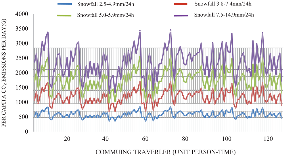
Carbon dioxide emissions from residents commuting at different levels of the snowstorm.

Figure 6.

Carbon dioxide emissions from residents commuting at different haze levels.

Discussion of Results

General characteristics of CCDE

Figures 4 to 6 illustrate the changes in carbon dioxide emissions caused by changes in commuting behaviors for urban residents under different rainstorms, snowstorms, and haze levels. Through the statistical analysis of the carbon dioxide emission data of residents’ commuting behavior in different extreme weather environments (see Table 8). As shown in Table 8, overall, under the influence of extreme weather the level of carbon dioxide emissions arising from travel by urban commuters is gradually decreasing. Under the rainstorm scenario, when the rainfall intensity is increased from 5.0–16.9 to 17.0–37.9 mm/24 hours, the total carbon dioxide emission intensity is reduced by 2.4%, and when the rainfall intensity reaches 50 mm/24 hours or more, the total carbon dioxide emission intensity is reduced by 3.5%. Under a snowstorm scenario, when the snowfall intensity is increased from 2.5–4.9 to 3.8–7.4 mm/24 hours, the total carbon dioxide emission intensity is reduced by 1.1%, and when it is increased to 5.0 to 9.9 mm/24 hours, the total carbon dioxide emission intensity is reduced by 2.1%. Moreover, when snowfall intensity is raised to 7.5 to 14.9 mm/24 hours, the total carbon dioxide emission intensity is reduced by 3.8%. Under a haze scenario, when the AQI is increased from 151–200 to 201–300, the total carbon dioxide emission intensity is reduced by 2.6%. Furthermore, when the level is increased to 300 or more, the total carbon dioxide emission intensity is reduced by 3.3% (see Table 8).

Table 8.

Characteristics of Carbon Dioxide Emissions Under Different Levels of Extreme Weather.

Statistical item	Rainstorm			Snowstorm				Haze
Statistical item	5.0–16.9 (mm/24 hours)	17.0–37.9 (mm/24 hours)	>50 (mm/24 hours)	2.5–4.9 (mm/24 hours)	3.8–7.4 (mm/24 hours)	5.0–9.9 (mm/24 hours)	7.5–14.9 (mm/24 hours)	151–200	201–300	>300
Maximum value (g)	882.39	856.45	840.32	844.43	861.56	873.72	885.32	881.59	996.45	882.34
Minimum value (g)	335.34	320.57	312.56	352.23	324.79	312.57	300.58	355.34	330.57	326.91
Average value (g)	601.76	587.27	580.91	596.64	590.47	584.41	573.79	602.82	587.42	582.73
Average reduction ratio (%)	—	2.4	3.5	—	1.1	2.1	3.8	—	2.6	3.3
<Average ratio (%)	45.67	49.71	48.39	47.41	48.54	46.59	47.89	46.77	48.68	49.28
>Average ratio (%)	54.33	50.29	51.61	52.59	51.46	43.41	52.11	53.23	51.32	50.72

Individual characteristics of CCDE

For convenience, we used A, B, and C to represent rainfall intensity levels of 5.0 to 16.9, 17.0 to 37.9, and >50 mm/24 hours, respectively; D, E, F, and G represent snowfall intensity levels of 2.5 to 4.9, 3.8 to 7.4, 5.0 to 9.9, and 7.5 to 14.9 mm/24 hours, respectively; while H, I, and J represent air pollution index levels of 151 to 200, 201 to 300, and more than 300, respectively. Under different extreme weather levels, carbon dioxide emissions from residents’ commuting showed different characteristics, as shown in Table 9.

(1) Under the rainstorm scenario, on the one hand, as the rainfall intensity continues to increase, the trend of decreasing carbon dioxide emissions from the residential commuters is the largest (accounting for 92.57%). This reflects the fact that most of the travelers gave up driving the car, or using public buses by choosing to use more environmentally friendly, low-emission forms of transportation such as the subway or by walking. In this instance, these changes are not directly affected by the weather events that are happening on the ground, which resulted in a sharp drop in carbon dioxide emissions as fewer people were using the roads to get around. However, on the other hand, 4.47% of the carbon dioxide emissions from commuting showed an increasing trend initially before then decreasing. This was due to the fact that some travelers chose to take a taxi when the amount of rainfall was relatively small. However, as the amount of rainfall increases, those travelers decided to use the subway or walk, which in turn reduced carbon dioxide emissions.

(2) Under the snowstorm scenario, as the intensity of snowfall continues to increase, in general, the proportion of declining trend of carbon dioxide emissions from the residential commuters is the largest (accounting for 95.23%), reflecting the fact that in heavy snow conditions, due to the impaired capacity of the, most travelers chose to use modes of transportation that had low-emission levels, such as the subway or by walking, which led to a sharp decline in carbon dioxide emissions. However, some of the results showed that in some instances carbon dioxide emission levels fluctuated up and down before than increasing again (1.21% of the sample). This may be due to the fact that some commuters choose high-emission forms of transportation such as the use of taxis in heavy snow conditions.

(3) Under the haze scenario, the change in carbon dioxide emissions from residential commuters is very different from the rainstorm and snowstorm scenarios. During hazy weather, the main factors affecting residents’ transportation behaviors are the government’s vehicle restriction measures (the ODPW and OAE). With the implementation of the vehicle restriction measures,51.83% of commuters changed their mode of transportation, giving up the use of private cars to then use low-carbon forms of transport such as subways, buses, or bicycles. Given this change, carbon dioxide emissions declined. However, 18.25% of commuters chose to use high emission forms of transportation, such as taxis or public buses. Moreover, about 12.69% of commuters owned a second car in their family, so they were able to avoid these vehicle restrictions by simply using the second vehicle, when their first choice of car was not able to be driven. Such actions caused the carbon dioxide levels to remain basically unchanged so that the effect of reducing carbon dioxide emissions together with other pollutants resulting from residents’ daily commuting was not achieved.

Table 9.

Changing of Carbon Dioxide Emissions During Extreme Weather Evolution.

Extreme weather scenario	Extreme weather trends	Changing trends in carbon dioxide	Proportion (%)
Rainstorm	A → B → C	Increasing	0.98
		Increasing first and then decreasing	4.47
		Decreasing	92.57
		Decreasing first and then increasing	1.98
Snowstorm	D → E → F → G	Increasing	0.74
		Increasing first and then decreasing	3.56
		Decreasing	95.23
		Decreasing first and then increasing	0.47
Haze	H → I → J	Increasing	18.25
		Increasing first and then decreasing	1.74
		Decreasing	2.18
		Basically unchanged	77.83

Note. A, B, and C represent rainfall intensity of 5.0 to 16.9, 17.0 to 37.9, and >50 mm/24 hours, respectively; D, E, F, and G represent snowfall intensity 2.5 to 4.9, 3.8 to 7.4, 5.0 to 9.9, and 7.5 to 14.9 mm/24 hours, respectively; and H, I, and J represent air pollution index 151 to 200, 201 to 300, and more than 300, respectively.

Conclusions

Although people are increasingly aware of the impact of weather on changes in travel behavior, the impact of extreme weather on carbon dioxide emissions from urban commuted is poorly understand. However, after understanding that extreme weather has an impact on commuter behavior, it is necessary to consider the emission factors of the alternative travel mode and the travel behavior to determine the exact changes in carbon dioxide emissions. Therefore, our study constructs a “W–B–C” analysis framework, by developing commuter transportation shift model that is based on the multiple logistic regression method to analyze the marginal impact of extreme weather on travel behavior based on the econometric models. By combining different methods of carbon dioxide emission factors and travel distance, the changes in carbon dioxide emissions from urban commuter travel under extreme weather conditions has been comprehensively analyzed.

This study collected 5,848 pieces of commuter travel data from Xi’an, China, which embodies the typical characteristics of winter, spring, and heating seasons. It also considers the probability that residents will change transportation mode due to various extreme weather events. At the same time, using a series of econometric models to describe the commuting travel behavior, we proposed the marginal effect of each extreme weather variable on various commuter transportation behavior variables. Through this analysis, the changing characteristics of carbon dioxide emissions caused by extreme weather changes can be obtained. The results illustrate the importance of extreme weather in the assessment of carbon dioxide emissions from residential commuters. In general, extreme weather events (rainstorms, snowstorms, and haze) gradually decrease the level of carbon dioxide emitted by urban commuters in Xi’an. However, the level of impact that governmental policies had under rainstorm, snowstorm, and haze conditions was different. With the increasing intensity of rainfall and snowfall, the level of carbon dioxide emissions from urban commuters fell 95.23% and 92.57% of the emissions for commuters in each category fell. As some travelers still chose to adopt high emission causing modes of transportation, such as taxis or ride-hailing in extreme weather, approximately 1.21% to 2.96% of CCDE recorded an increasing trend. Unlike the recorded results of rainstorms and snowstorms, in the haze scenario, the vehicle restriction policy only reduced the CCDE by 2.18%, with 77.83% of the CCDE remaining unchanged. This is because some travelers adopt high emission generating modes of transportation such as taxis or ride-sharing. Moreover, at the same time, about 12.69% of the travelers owned a second car, and as such they were able to get around the vehicle restriction requirements. As a result, most of the CCDE remain basically unchanged and the emission reduction effect has not been achieved. Therefore, due to the large-scale haze in during the hot season in Northern China, some cities will adopt dynamic vehicle restriction methods to reduce the emission of carbon dioxide and other pollutants. However, as can be seen from the results of this study, the effect of this measure is not obvious. On the one hand, government policies should focus on the market promotion and use of new energy vehicles, and on the other hand, strengthen publicity through the use of modern information transmission to improve the public’s awareness of low carbon emission reduction, and regulate the public’s choice of travel behavior through taxation, credit, and subsidies. The urban traffic management department should formulate traffic emergency plans that are specifically targeted for extreme weather events, particularly those that increase the use of bus and rail transit, and improve the emergency response capacity of public transportation networks during extreme weather events. The results of which will greatly reduce carbon dioxide emission levels from urban commuter travel.

This study also has certain limitations. First, this study uses tracking data from emerging national central cities in China-Xi’an city. Although it covers the data from different time periods and different types of extreme weather, this data source is also limited. Considering extreme weather factors, it is best to use large-scale supply and demand models to analyze further results in the future. Second, the marginal effects of extreme weather variables may vary depending on the climate conditions experienced across the different regions, while this study mainly analyzes the impact of extreme weather events on carbon dioxide emissions from residential commuters in Xi’an, China, the results may not be applicable to other regions and countries with different climatic conditions. In addition, this study mainly considers the characteristics of direct carbon dioxide changes generated during shifts in choice of transportation mode from urban commuters has not considered the carbon emissions from non-residential (or heavy industry, i.e., trucks, etc.) travel behaviors, and due to logistics and transportation. As well know, China’s economic development is closely related to logistics and transportation (Wang et al., 2021). These problems may become the focus of subsequent studies in the future.

Footnotes

Declaration of Conflicting Interests

The author(s) declared no potential conflicts of interest with respect to the research, authorship, and/or publication of this article.

Funding

The author(s) disclosed receipt of the following financial support for the research, authorship, and/or publication of this article: This study was supported by National Social Science Foundation of China (No. 20BJY179), Research Project on Major Theoretical and Practical Problems of Philosophy and Social Sciences in Shaanxi Province, China (No. 2021ND0447), the Fundamental Research Funds for the Central Universities, China (CHD No. 300102231666), Annual Scientific Research Program for Youth Innovation Team Construction of Shaanxi Provincial Department of Education, China (No. 21JP005), Social Science Planning Foundation of Xi’an city, China (No. 22JX197), and Social Science Foundation of Shaanxi Province, China (No. 2022D138).

ORCID iD

Chao Wang

References

Abenoza

R. F.

Liu

Cast

(2019). What is the role of weather, built-environment and accessibility geographical characteristics in influencing travelers’ experience? Transportation Research Part A: Policy and Practice, 122, 34–50.

AI Duhayyim

Albraikan

A. A.

Rizwanullah

. (2022). Modeling of artificial intelligence based traffic flow prediction with weather conditions. Computers Materials & Continua, 71(2), 3953–3968.

Ben

Kiron

Steve

(2016). Changes to commute mode: The role of life events, spatial context and environmental attitude. Transportation Research Part A: Policy and Practice, 89, 89–105.

Böcker

Prillwitz

Dijst

(2013). Climate change impacts on mode choices and travelled distances: A comparison of present with 2050 weather conditions for the Randstad Holland. Journal of Transport Geography, 28, 176–185.

Brand

Goodman

Rutter

(2013). Associations of individual, household and environmental characteristics with carbon dioxide emissions from motorized passenger travel. Applied Energy, 104, 158–169.

Brand

Preston

J. M.

(2010). ‘60–20’ emission-the unequal distribution of greenhouse gas emissions from personal, non-business travel in the UK. Transport Policy, 17(1), 9–19.

Cervero

(1996). Mixed land-uses and commutings: Evidence from the American Housing Survey. Transportation Research Part A: Policy and Practice, 30(5), 361–377.

Chai

Y. W.

Xiao

Z. P.

Liu

Z. L.

(2012). Low–carbon optimization strategies based on CO₂ emission mechanism of household daily travels: A case study of Beijing. Geographical Research, 31(2), 334–344.

Chen

Zhang

J. Q.

Jiang

X. Y.

(2012). Scenario simulation-based assessment of trip difficulty for urban residents under rainstorm waterlogging. International Journal of Environmental Research and Public Health, 9(6), 2057–2074.

10.

Chen

Shahabi

Zhang

(2018). Landslide susceptibility modeling based on GIS and novel bagging-based kernel logistic regression. Applied Sciences, 8(12), 2540.

11.

Chowdhury

Dey

Tripathi

S. N.

Beig

Mishra

A. K.

Sharm

(2017). “Traffic intervention” policy fails to mitigate air pollution in megacity Delhi. Environmental Science and Policy, 74, 8–13.

12.

de Kuijf

Waerden van der

Dijst

. (2021). Integrated weather effects on e-cycling in daily commuting: A longitudinal evaluation of weather effects on e-cycling in the Netherlands. Transportation Research Part A: Policy and Practice, 148, 305–315.

13.

Dijst

Böcker

Kwan

M. P.

(2013). Exposure to weather and implications for travel behavior: Introducing empirical evidence from Europe and Canada. Journal of Transport Geography, 28(1), 24–26.

14.

Feng

(2016). Risk factors affecting fatal bus accident severity: Their impact on different types of bus drivers. Accident Analysis & Prevention, 86, 29–39.

15.

Ferri-Garcia

Fernandez-Luna

J. M.

Chillon

(2020). Data mining techniques to analyze the factors influencing active commuting to school. International Journal of Sustainable Transportation, 14(4), 308–323.

16.

Lam

W. H. K.

Meng

(2014). Modelling impacts of adverse weather conditions on activity–travel pattern scheduling in multimodal transit networks. Transportmetrica B: Transport Dynamics, 2(2), 151–167.

17.

Gong

Y. X.

G. C.

Lin

Y. Y.

Duan

Z. Y.

(2013). Impact of land use on urban household travel carbon emissions. Urban Development Studies, 20(9), 111–118.

18.

Huang

J. C.

Lin

H. X.

(2017). Spatial evolution analysis and multi-scenarios simulation of Beijing-Tianjin-Hebei urban agglomeration. Geographical Research, 36(3), 506–517.

19.

Huang

Liu

Cao

(2015). Commuting carbon emission characteristics of community residents of three spheres: A case study of three communities in Guangzhou city. Geographical Research, 34(4), 751–761.

20.

Koetse

M. J.

Rietveld

(2009). The impact of climate change and weather on transport: An overview of empirical findings. Transportation Research Part D: Transport and Environment, 14(3), 205–221.

21.

Lin

P. F.

Weng

J. C.

Yin

B. C.

(2020). Analysing the relationship between weather, built environment, and public transport ridership. IET Intelligent Transport Systems, 14(14), 1946–1954.

22.

Liu

C. Q.

Shi

N. N.

Zhu

L. C.

(2017). Transferability of commute behavior across different spaces within metropolis. Journal of Transportation Systems Engineering and Information Technology, 17(13), 206–212.

23.

Liu

C. Q.

Susilo

Y. O.

Dharmowijoyo

(2018). Investigating intra-household interactions between individuals’ time and space constraint. Journal of Transport Geography, 73, 108–119.

24.

Liu

C. Q

Susilo

Y. O.

Karlström

(2015a). The influence of weather characteristics variability on individual’s travel mode choice in different seasons and regions in Sweden. Transport Policy, 41, 147–158.

25.

Liu

C. Q.

Susilo

Y. O.

Karlström

(2015b). Investigating the impacts of weather variability on individual’s daily activity-travel patterns: A comparison between commuters and non-commuters in Sweden. Transportation Research Part A: Policy and Practice, 82, 47–64.

26.

Liu

C. Q.

Susilo

Y. O.

Karlström

(2015c). Measuring the impacts of weather variability on home-based trip chaining behavior: A focus on spatial heterogeneity. Transportation, 43(5), 843–867.

27.

Liu

C. Q.

Susilo

Y. O.

Karlström

(2016). Estimating changes in transport CO2 emissions due to changes in weather and climate in Sweden. Transportation Research Part D: Transport and Environment, 49, 172–187.

28.

Liu

Z. Y.

R. M.

Wang

X. K.

Shang

(2017). Effects of vehicle restriction policies: Analysis using license plate recognition data in Langfang, China. Transportation Research Part A: Policy and Practice, 118, 89–103.

29.

National Meteorological Information Center. (2021). Retrieved December 20, 2021, from http://data.cma.cn/

30.

Romano

L. G.

Johannesson

Fredrik

Jacobson

(2021). An enhanced stochastic operating cycle description including weather and traffic models. Transportation Research Part D, 97, 102878.

31.

Seo

Shim

Seo

(2018). Underwater cylindrical object detection using the spectral features of active sonar signals with logistic regression models. Applied Sciences, 8(1), 116.

32.

Shaanxi Provincial Meteorological Bureau. (2021). Retrieved December 20, 2021, from http://sn.cma.gov.cn/

33.

Sheyda

Roorda

J. M.

Kennedy

(2012). Modelling the impact of weather conditions on active transportation travel behavior. Transportation Research Part D: Transport and Environment, 17, 129–137.

34.

Sikder

Wang

Yao

X. X.

Huai

L. M.

Yeboah

F. K.

Wood

Zhao

Y. L.

Dou

X. C.

(2022). The integrated impact of GDP growth, industrialization, energy use, and urbanization on CO₂ emissions in developing countries: Evidence from the panel ARDL approach. Science of the Total Environment, 837, 155795. https://doi.org/10.1016/j.scitotenv.2022.155795

35.

Simone

Lin

Richard

(2018). The potential implications of autonomous vehicles in and around the workplace. International Journal of Environmental Research and Public Health, 15, 1–19.

36.

Wang

Kim

Y. S.

Kim

C. Y

. (2021). Causality between logistics infrastructure and economic development in China. Transport Policy, 100, 49–58.

37.

Wang

Wood

Geng

X. R.

Wang

Y. J.

Long

X. L.

(2020). CO₂ emission in transportation sector across 51 countries along the Belt and Road from 2000 to 2014. Journal of Cleaner Production, 266, 122000.

38.

Wang

Wood

Geng

X. R.

Wang

Y. J.

Qiao

C. Y.

Long

X. L.

(2020). Transportation CO₂ emission decoupling: Empirical evidence from countries along the belt and road. Journal of Cleaner Production, 263, 121450.

39.

Wang

Zhao

Y. L.

Wang

Y. J.

Wood

Kim

C. Y.

(2020). Transportation CO₂ emission decoupling: An assessment of the Eurasian logistics corridor. Transportation Research Part D: Transport and Environment, 86, 102486.

40.

Jiang

Shen

Yang

(2018). Gene selection in cancer classification using sparse logistic regression with L_1/2 regularization. Applied Sciences, 8(9), 1569.

41.

Xi’an Real-time Air Quality Index. (2021). Retrieved December 20, 2021, from http://aqicn.org/city/xian/cn/

42.

Yang

W. Y.

Liang

F. W.

Cao

X. S.

(2020). Examining the effects of the multi-scale built environment on residents’ CO₂ emissions from commuting: An empirical study of Guangzhou. Geographical Research, 39(7), 1625–1639.

43.

Y. C.

Wang

Y. J.

Y.Q.

(2021). Impact of urban density on carbon emissions in China. Applied Economics, 53(53), 6153–6165.

44.

Zanni

Ryley

T. J.

(2015). The impact of extreme weather conditions on long distance travel behavior. Transportation Research Part A: Policy and Practice, 77, 305–319.

45.

Zhang

Han

Z. L.

Chen

Y. Y.

J. X.

Cui

(2018). A model of highway travelers’ travel mode shift under rainy weather. Journal of Highway and Transportation Research and Development, 35(6), 105–111, 130.

46.

Zhang

X. Y.

Yang

X. M.

Yan

(2014). Statistical estimation method for energy consumption and carbon emissions by urban transport. China Soft Sciences, 6, 142–150.

47.

Zhao

H. R.

Chen

(2016). Application of improved MOPSO in logistics node location model. Computer Engineering and Applications, 52(12), 239–245.

Extreme Weather Influence on Carbon Emissions in Chinese Urban Traffic Environments

Abstract

Keywords

Introduction

The Analysis Framework

Research Model

Transportation Mode Shift Model

Marginal Effect of Extreme Weather on Residents’ Commuting Travel Behaviors

Changes in Carbon Dioxide Emissions From Commuter Transportation, Under an Extreme Weather Scenario

Variable Selection

Research Area and Data Sources

Empirical Research

Analysis of the Impact of Extreme Weather on Residents’ Commuting

Changes Analysis of Carbon Dioxide Emissions

Discussion of Results

General characteristics of CCDE

Individual characteristics of CCDE

Conclusions

Footnotes

Declaration of Conflicting Interests

Funding

ORCID iD

References