Sage Journals: Discover world-class research

Abstract

The accumulation of properties by Spanish banks during the crisis of the first decade of the 21st century has definitely changed the housing market. An optimal house price valuation is useful to determine the bank’s actual financial situation. Furthermore, properties valued according to the market can be sold in a shorter span of time and at a better price. Using a sample of 24,781 properties and a simulation exercise, we aim to identify the decision criteria that Spanish banking used to decide which properties were going to be sold and at what price. The results of the comparison among four methods used to value real estate—artificial neural networks, semi log regressions, a combined model by means of weighted least squares regression, and quantile regressions—and the actual situation suggest that banking aimed to maximize the reversal of impairment losses, although this would mean capital losses, selling less properties, and decreasing their revenues. Therefore, the actual combined result was very detrimental to banking and, consequently, to the Spanish society because of its banking bailout.

Keywords

artificial neural networks hedonic prices banking real estates housing Spain

Introduction

Financial institutions are big players in the Spanish housing market. This has been particularly evident during and after the financial crisis of the first decade of the 21st century, given many foreclosed properties were acquired by financial institutions because of both evictions and bankruptcies of construction companies (Cano et al., 2013). In this regard, Gutiérrez & Domenech (2017) conclude that “as a result of the massive wave of evictions, banks have emerged as large-scale property owners in Spain and key agents for present and future housing policies.”

The emergence of a new accumulation regime in the housing market by the banking industry in Spain since the early 2000s is a case of financialization (Zwan, 2014). Aalbers (2008) concludes that housing is a central aspect of financialization given that homes and homeowners became considered to be financially exploitable. Rolnik (2013) suggests that there has been all around the world a change in housing and urban policies due to globalization and neoliberalism, which has generated a new paradigm mainly focused on the implementation of policies to commoditize housing so as to contribute to the financialization of the real estate market. There is an abundance of literature about housing and financialization: Fernández and Aalbers (2016), Smart and Lee (2003), Fields (2017), Wainwright and Manville (2017), Wijburg and Aalberts (2017), Çelik (2021), Migozzi (2020), and Fernández and Aalbers (2020) among others. And some of them have analyzed the Spanish case: Garcia-Lamarca and Kaika (2016), Coq-Huelva (2013), Palomera (2014), and Byrne (2020).

Nonetheless, for the time being, no paper has analyzed the decision criteria that Spanish banks used to sell the properties they had accumulated during the crisis. To achieve it, we compared the results of the making decision criteria actually used by banking with the results obtained using three methods to value real estate, namely artificial neural networks (ANN), semi log regressions (SLR), and quantile regressions (QR; Torres-Pruñonosa et al., 2021). Hedonic regression models (SLR and QR) have been selected to be applied to this paper given that they have been extensively used by academia to analyze housing prices (Chin & Chau, 2003; Owusu-Ansha, 2011). In regard to SLR hedonic models, Follain and Malpezzi (1980) highlight different advantages in their use, such as helping to alleviate the heteroscedasticity problem. In regard to QR models, Zietz et al. (2007) point out as their advantage that the truncation problem is avoided because they use the entire sample and, therefore, the biased estimates created by SLR is eliminated. Nonetheless, since housing scholars do not agree in regard to the functional form to be used, we have considered it appropriate to complement hedonic models with ANN, taking into account that the latter have been also widely used by scholars in price housing studies and there is an abundant and solid scientific literature that validates its use in housing (see Section 3). Additionally, a fourth method resulting from the combination of ANN and SLR by means of a weighted least squares (WLS) regression has also been applied, because independent information is given by ANN and SLR models in view that they process data differently (Terregrosa & Ibadi, 2021).

Therefore, the aim of this paper is to identify the decision criteria that Spanish banking used to decide which properties were going to be sold and at what price. Analyzing the decision-making criteria used by Spanish banks will contribute to the understanding of how they shaped the housing market, converting it into a mere commodity to be financially exploited.

In this sense, ANN, SLR, QR, and WLS regression models have been applied to a sample of one Spanish bank’s sold and unsold properties, which was the result of the merger of three savings banks and the forecasting skill has been compared to the transaction prices. Furthermore, a simulation exercise is presented in which has been estimated the increase of revenues the bank would obtain in case of using the most appropriate methodology. According to the results obtained, if the proposed methods had been used in order to determine the value and the consequent selling strategy of these assets, an increase in revenues and a better combined outcome—on the grounds of both capital gains and losses obtained and the impairment losses not deleted after the selling—in comparison to the actual situation would have been obtained.

The structure of the paper is the following: Section 2 analyses the Spanish real estate bubble and how the banking industry was affected. In Section 3 the methodology applied, as well as the datasets used and the variables analyzed are described. Thereafter, in Section 4 the results are shown and discussed. Finally, the conclusions and proposal for further research are presented in Section 5.

The Spanish Case

Spain experienced an outstanding housing boom in the period between 1998 and 2007 (Raya et al., 2017), increasing both the number of houses constructed and mortgages contracted. Take the example of 2006, when 860,000 dwellings were started. Likewise, with an annual average of 15.5 million dwellings during the boom years, an average of 1.1 million mortgages were contracted annually.

In this context, banking managers were pressured to increase the number of new mortgages so as to increase profits. Furthermore, prices were inflated during the boom period because appraisers’ incentives were distorted. Appraisers were incentivized to inflate their appraisal prices in order to satisfy banks, so as to receive more appraisal assignments. Akin et al. (2014) estimate the overappraisal mean at around 30%. When housing prices increase, if expectations are bullish, drawing larger mortgages may not appear to increase risk (Hott, 2015). For this reason, during housing boom years, financial institutions are eager to open the market for financially constrained borrowers. As mentioned earlier, to do so, appraisers were encouraged to bias upwardly their appraisal prices. Given that the appraisal price was used by banking to calculate the loan-to-value (LTV) ratio, the artificially appraisal increase allowed granting larger mortgages (Duca et al., 2010) and interest rates.

Finally, the Spanish housing market collapsed. Spain was affected by the financial crisis more severely than other developed countries due to both the excessive dependence on the real estate industry and the softening of the credit standards (Akin et al., 2014).

Consequently, one of the main problems for financial institutions was that risky mortgages as well as properties with inflated prices were registered on their balance sheets. The vast majority of the housing stock from financial institutions came from foreclosures (in the case of family properties) or, especially, bankruptcy (in the case of properties from construction companies). To illustrate, using the net value of properties assets (16,929 million euros) provided by the financial institutions as well as information of the properties sold, we estimate that the amount of dwellings in the balance sheet of the financial institutions at the end of 2013 was 245,000. This figure represented 28.8% of the housing stock. In this scenario, financial institutions created subsidiaries that acted as real estate broker companies in order to sell housing stock. The following companies are examples: Altamira Asset Management, S.A. (created in 2013 by Banco Santander), Haya Real Estate, S.L. (created in 2013 by Bankia), and Aliseda Inmobiliaria Servicios de Gestión Inmobiliaria S.L. (created in 2014 by Banco Popular). These companies are responsible for a higher portion of housing transactions. Unlike traditional real estate agents, these companies own the dwellings and in consequence their incentives are to maximize selling prices (Hendel et al., 2009; Levitt & Syverson, 2008).

Finally, banks were forced by the Bank of Spain to register impairment losses. As a consequence, most savings banks were merged and transformed into commercial banks (San-José et al., 2020) and the Spanish banking system was bailed out: 61,495 million euros were needed. A large part of this bailout can be explained by the inflated appraisal values.

All in all, real estate crisis left a large proportion of dwellings at inflated prices on the balance sheets of many banks. In this regard, the banking industry needed to face the challenge of how to find a way to value their real estate stock. If the valuation were accurate, it would help to assess the actual financial situation of the bank and, given that the real estate would be valued according to the market, it would allow to sell properties more quickly and at a higher price. Therefore, the best way to value the properties stock would be the one that reduces the selling time since it assesses properly the market value. We aim to identify what criteria were used by banking when selling the real estates accumulated during the crisis.

Methodology

Hedonic analysis has been commonly used in order to deal with quality heterogeneity to value housing. Hedonic models are applied to explain the price of non-homogenous products. They note that the implicit marginal price of their heterogonous characteristic can be calculated by means of estimating models, which can explain the price on the basis of their characteristics. Court (1941) is considered to be the first hedonic price methodology paper. The inception of economic literature on hedonic prices has the car market as its framework: Griliches (1971) used this methodology to estimate car prices once the characteristics that affected them were controlled, for instance, horsepower or the consumption of fuel. Previously, the technique was popularized by Tinbergen (1951) who established the theoretical framework, and Rosen (1974), who provided a theoretical foundation that showed that the characteristics of heterogeneous products determine implicitly marginal prices. The modern consumer choice theory, according to which the consumer derives utility not directly from the good but from its features (Lancaster, 1966), is the basis of the hedonic technique. Given that each and every house is a different product with unique characteristics, real estates are products that perfectly fit into the framework of hedonic price models. For this reason, there are many examples of outstanding hedonic studies of the housing market: Bartik (1987), Bin (2006), Bover and Velilla (2002), García and Raya (2011), Mendelsohn (1984), Mills and Simenauer (1996), and Palmquist (1984). Over the last years, this methodology has been widely applied to analyze the determinants of housing price, such as air quality (Li et al., 2016), energy efficiency (Bisello et al., 2019; De Ayala et al., 2016; Fuerst et al., 2015) environmental amenities (Chen et al., 2017; Wu et al., 2017), service amenities (Li et al., 2019), and transportation accessibility (Geng et al., 2015; Yang et al., 2020) among others. Jayantha and Oladinrin (2019) carry out a co-citation bibliometric analysis of hedonic price models literature and reveal that the research areas that have most attracted the attention of academia are housing state, economic return and neighborhood parks.

In order to calculate hedonic models, equation (1) needs to be estimated:

P_{i t} = β_{0} + \sum_{k = 1}^{k = K} β_{k} X_{i k} + \sum_{l = 1}^{l = L} α_{l} D_{l} + \sum_{t = 1}^{t = T} δ_{t} D_{t} + e_{i t}

(1)

where the aim is to try to explain the price of a dwelling ( $P_{i t}$ ) based on its characteristics ( $X_{i k}$ ), the postal code in which it is located ( $D_{l}$ ), and the year ( $D_{t}$ ) in order to know the time trend. Lastly, $β_{k}, α_{l} and δ_{t}$ are parameters and $e_{i t}$ is the disturbance term, which follows the usual assumptions.

Thus, the hedonic price theory supports the application of this regression model and allows calculating the homogeneous parameters of real estates. When it comes to the housing context, it is evident that the price of dwellings is a differentiating factor in the valuations made by individuals with regard to their physical characteristics. For this reason, we aim to find out the price distribution along with the explanatory variables’ behavior.

In SLR model, ordinary least squares (OLS; Gujarati & Porter, 2010) were used to calculate hedonic equations which parameters aims to minimize the residual ( $e_{i t}$ ) of the econometric model shown in equation (1) as follows:

\sum {(e_{i t})}^{2} .

(2)

Quantile regressions (QR) can also be used to estimate hedonic prices. When the links between the dependent variable and the explanatory ones throughout the entire distribution of the former cannot be captured by means of estimating conditional mean, QR are often used. For instance, a median-based estimator can be appealing, in view that it is less sensitive to outliers than a mean-based estimator obtained by means of SLR. Thus, the bias from unobserved characteristics should be smaller. Many are the papers that have used QR on housing: Coulson and McMillen (2007), Garcia and Raya (2015), McMillen (2008), McMillen and Thorsnes (2006), Nicodemo and Raya (2012), Fernández and Bucaram (2019), and Torres-Pruñonosa et al. (2021). In regard to the application of QR on housing, some papers analyze the determinants of house prices, such as housing characteristics (Ebru & Eban, 2009; Mora-García et al., 2019), environmental amenities (Czembrowski et al., 2016; Fernández & Bucaram, 2019; Trojanek et al., 2018; Tuofu et al., 2021), environmental hazards (Mueller & Loomis, 2014), air pollution (Chasco & Le Gallo, 2015), transport accessibility (Wen et al., 2018; Yang et al., 2020), hospital’s proximity (Peng & Chiang, 2015), educational facilities (Wen et al., 2019), and crime perception (Buonanno et al., 2013; Wilhelmsson & Ceccato, 2015) as well as other amenities (Cui et al., 2018; McCord et al., 2018). Kang and Liu (2014) use QR to analyze the impact of financial crisis on housing prices and Torres-Pruñonosa et al. (2021) the use of QR by banks in mass appraisal in housing.

In a QR (Buchinsky, 1998), the target quantile (q) from the distribution residuals is a parameter that is specified before the estimation. Therefore, the quantile parameter estimates are the coefficients that minimize Equation 3:

\sum_{e_{i t} > 0} 2 q | e_{i t} | + \sum_{e_{i t} < 0} 2 (1 - q) | e_{i t} |

(3)

For example, at the median (the 50th quartile or q = 0.5), equal weights are assigned to positive and negative residuals. Nonetheless, in the case of the 75th percentile (q = 0.75), positive residuals are given more weight. Therefore, equation (3) will be minimized to a set of parameter values in which 100q% of the residuals are positive. Classically, this criterion is known as minimum absolute deviations. In this regard, the Koenker and Bassett (1978) algorithm is commonly employed.

In regard to QR model, we have estimated quantile 10th, 25th, 50th, 75th, and 90th. There is no consensus among scholars in regard to the selection of percentiles used when conducting QR on housing studies. Among many options (Hodge, 2016; McMillen & Shimizu, 2020), some authors use only the quartiles (Okkola & Brunelle, 2018; Zhang & Yi, 2018) whereas others use the deciles (Liao & Wang, 2012; Zietz et al., 2007). Combining both approaches and using the same criteria of Chen et al. (2007), Zahirovich-Herbert and Gibler (2014), and Mora-Garcia et al. (2019), the quantile regression was carried out for three quartiles (the 25th, the 50th, and the 75th quantile) as well as for the first decile (the 10th quantile which represent the bottom segment) and the last decile (the 90th quantile which represent the top segment).

There is no consensus also among scholars in regard to the linearity of hedonic function. Although some studies use the linear-hedonic function (Baen & Guttery, 1997; Rossini et al., 1993), others use a nonlinear function, such as the early work of Palmquist (1984). In this same line, Sheppard (1999) bases his research on the nonlinearity of the hedonic equation and Ekeland et al. (2002) support the idea that in the hedonic model nonlinearity is a generic property of equilibrium. In order to take into account the approach that considers that the hedonic price function is a nonlinear function and, therefore, the marginal implicit price is an endogenous variable of it, we will also use artificial neural networks (ANN) to be able to assess the nonlinear structure. Another solution would be to choose a nonlinear specification that is suitable for the hedonic price function. In this regard, Ekeland et al. (2002) consider that, if the marginal price function is nonlinear, the demand parameters are always identified in single market data. Ekeland et al. (2004) affirm that the linearization of the hedonic model can produce identification problems, concluding that the hedonic model is nonlinear. Goodman (1978) states that there is no theoretical basis for a priori determination of the functional form of the hedonic model and chooses multiplicative models instead of linear forms.

There is abundant literature about ANN assessing real estates. The first paper to apply ANN to this industry was written by White (1988). In it, there is a comparison between ANN and traditional methods. Other authors showed that ANN perform better (Do & Grudnitski, 1992; Kauko, 2003; Landajo et al., 2012; Limsombunchai, 2004; Peter et al., 2020; Peterson & Flanagan, 2009; Tay & Ho, 1992). Selim (2009) shows that ANN are better predictors than traditional models. Nevertheless, Curry et al. (2002) and McGreal et al. (1998) demonstrated that standard hedonic regressions work as well as ANN. Some authors show that the performance of ANN is conditional on the use of certain variables (Do & Grudnitski, 1993; Liu et al., 2006; McGreal et al., 1998; Nghiep & Cripps, 2001; Peterson & Flanagan, 2009). Nonetheless, Worzala et al. (1995) show that ANNs are better only in the case of a very homogeneous data sample, in which all houses belong to the same postal code. From this point, there are more papers that reach the same conclusion (Lenk et al., 1997; McCluskey et al., 2013). There are different authors who have used machine learning algorithms to obtain house price predictions. (Park & Bae, 2015). Other authors make comparisons of these algorithms with other models, including neural networks (Baldominos et al., 2018). Moreno-Izquierdo et al. (2018) compare the results of neural networks and hedonic regression models to achieve price optimization. Their conclusions are that neural networks achieve better estimates than hedonic regression models. Kang et al. (2020) reach the same conclusion, concluding that neural networks are a good method to calculate the prices of residential houses. In his study, he compares neural networks with genetic algorithms. In some studies, neural networks conclude that location is the key variable in the formation of house prices (Chiarazzo et al., 2014). Ambika et al. (2020) assess the present status of the market using multi-level models and ANN to demonstrate house costs. This undertaking presents the advancement of a multi-layer neural system based models to help land financial specialists and home designers in this basic assignment.

Neural networks are mathematics algorithms based on the way biological neurons compute information. There are different families of neural networks and the most well-known are the supervised neural networks—commonly known as ANN—which are universal proxies of functions; if there are any relations between two sets of data, the ANN find the algorithm that links both.

The basic unit of a ANN is the artificial neuron which is a node that receives information from other neurons, that are the variables of the model. The information that receives the neuron is averaged by synaptic weights which are calculated by the model. Equation (4) is the sum of the multiplications of each variable of the model by synaptic weights of each variable which is received by the neural network.

H = \sum_{i = 1}^{N} X_{i} W_{i} .

(4)

where X_i is the value of the variable and W_i is the synaptic that link variable i with the neuron. If the result of this calculus is higher than a number called bias, a transfer function to modify this result is used which can be either linear or sigmoid. The result of this function will be the result of the artificial neuron. For instance, if an artificial neuron has a log sigmoid transfer function, the result of the function would be the following algorithm (equation (5)):

Y_{j} = \frac{1}{1 + e^{- (\sum_{i = 1}^{N} X_{i} W_{i} + θ)}} .

(5)

where θ is the bias, X_i is the value of the variable i, W_i is the synaptic weight that links the variable i with neuron j, and Y_i is the answer of neuron j.

An artificial neuron is not able to make a logical process, but a set of artificial neurons can; therefore, neurons are grouped in networks to make logical calculus. Neural networks have layers and, usually, a typical neural network has three layers: the first one is the input data layer, the second one is a hidden layer where the data is processed, and the last one is the output result layer. Depending on the kind of research to be carried out by the analyst, the design may change, in particular in regard to the number of neurons in each layer. Each and every neuron of layers is linked with each and every neuron of the next layer. Thus, when a neuron computes a result, it is sent averaged by synaptic weight to each and every neuron of the next layer.

Figure 1 shows a representation of a three-layer neural network. In this example, X₁ and X₂ are two input data variables that send information to each and every hidden layer neuron. Therefore, the number of links between input data variables and the hidden layer is equal to the number of neurons of the latter. In our example, two input data variable are linked to three hidden layer neurons; consequently, these three hidden layer neurons receive two information flows from two input data variables which are averaged by synaptic weights.

Figure 1.

Neural network with two input data neurons, three hidden ones, and one output data neuron [2–3–1].

The mathematic process previously described occurs within the hidden layer neuron. The reaction of each and every neuron is to send data averaged by synaptic weight to the output data layer. The same process runs in the output data layer and, finally, the output of the net will be the result of the output data layer neuron.

If neural networks are trained, by means of introducing data and the expected result by the analyst, they can find non-linear links between two datasets. Neural networks use the learning algorithms several times, changing the weights—initially values are assigned randomly–in order to find the set of weights that minimize the forecast error. This kind of net is called supervised, given that during the training the result is compared with target data. The differences are used to modify the synaptic weights to decrease the error.

The most used neural network is called Multi-Layer Perceptron (MLP; Saeidi et al., 2017). This kind of ANN is considered as a universal function approximation. This is a multiple-layer net—usually a three-layer net (input data, hidden, and output data)—and uses a sigmoid transfer function in the hidden layer and a linear or sigmoid transfer function in the output data, depending on the expected result. The main characteristic of MLP is the use of a learning function called back-propagation or BP rule. This algorithm computes during the training process the error and changes the synaptic weights of the previous layer to decrease the error. Initially, BP changes output weights and, thereafter, it back-propagates to the hidden layer, changing their weights. This process may iterate so as to obtain the minimum error between the set of results and the target data.

All in all, the ANN used in this paper is a MLP with 15 neurons in both the input and hidden layer as well as 1 neuron in the output layer. Whereas the transfer function in the hidden layer is tan-sigmoid, the one in the neuron of the output layer is linear. The training algorithm is the back-propagation algorithm with the Levenberg–Marquardt algorithm with an early stop to avoid the over-training.

The combination of different forecast models aims to reduce the bias of individual models and improve their forecasting performance (Bates & Granger, 1969; Terregrossa, 2005; Timmermann, 2006). In this regard, some papers used combination forecast of prices applied to real estates by means of combining housing models, with different approaches, and improving the forecasting accuracy in comparison with their components (Gupta et al., 2011; Cabrera et al., 2011; Alexandridis et al., 2018). In particular, Terregrossa and Ibadi (2021) combines hedonic models and ANN by means of a restricted WLS regression–to overcome heteroscedasticity–using the inverse of component model forecast errors as forecast weights (Drought & McDonald, 2011) which increases the forecasting accuracy over hedonic and ANN model. Following Terregrossa and Ibadi’s (2021) approach, we have used a WLS regression to combine the SLR and ANN models by means of estimating equation (6):

P_{i t} = α + β [{\hat{P}}_{i t} (S L R)] + γ [{\hat{P}}_{i t} (A N N)] + e_{i t} .

(6)

where $P_{i t}$ is the price of a dwelling, ${\hat{P}}_{i t} (S L R)$ are the forecasts generated by the SLR model, ${\hat{P}}_{i t} (A N N)$ are the forecasts generated by the ANN model, $α, β, γ$ are parameters and $e_{i t}$ is the error term. If the estimated $\hat{β}, \hat{γ}$ parameters are different to zero, it can be assumed that SLR and ANN models have independent information useful to be combined (Terregrossa & Ibadi, 2021). In regard to WLS regression restrictions, two variations have been applied, namely with a constant term a with a suppressed constant term.

Two datasets have been analyzed, which included properties located in Catalonia. The first one, dataset I was provided by a Spanish commercial bank that formerly was a savings bank resulting from the merger of three savings banks. This financial institution was the owner of the properties as a consequence of foreclosures and the bankruptcies of construction companies. All properties in dataset I were valued by independent appraisals companies. The time period for the dataset is 2004 to 2013. Finally, dataset II is a sample of dataset I, which consists of 5,334 properties from 2004 to 2013 whose transaction prices are also included. Hence, the price variable consists of independent real estate appraisals for dataset I and both appraisal and transaction prices for dataset II. The natural logarithm has been used in all cases. When it comes to explanatory variables, nine dwelling characteristics or hedonic variables, year and postal code have been used. In Table 1 these variables are shown in detail, as well as their definitions, whereas Table 2 shows the descriptive statistics.

Table 1.

Definition.

Variable	Type	Definition
Ln (Price_A)	Quantitative	Natural logarithm of the appraisal price
Ln (Price_T)	Quantitative	Natural logarithm of the transaction price (online available for dataset II)
Ln (Price_O)	Quantitative	Natural logarithm of the offer price (online available for dataset II)
Height	Qualitative	The height of the house
Elevator	Dichotomous	Whether the access to the house is by means of an elevator (1 = yes, 0 = no)
Heating	Dichotomous	Whether the house use a heating system (1 = yes, 0 = no)
Pool	Dichotomous	Whether the house or the residents’ association property include a swimming pool (1 = yes, 0 = no)
Gardens	Dichotomous	Whether the house or the residents’ association property include gardens (1 = yes, 0 = no)
Size	Quantitative	Constructed square meters of the house
Condition	Dichotomous	Physical state of the house meaning (1 = good, 0 = bad)
Baths	Quantitative	Number of baths per house
Rooms	Quantitative	Number of rooms per house
PC	Qualitative	Postal Code
Year_A	Quantitative	Year where the house is appraisal priced
Year_T	Quantitative	Year where the house is transaction priced
Year_O	Quantitative	Year where the house is offer priced

Table 2.

Descriptives.

Variable1	Dataset I		Dataset II
Variable1	M	SD	M	SD
Ln (Price_A)	11.839	0.553	12.031	0.490
Ln (Price_T)			11.613	0.581
Ln (Price_O)			11.876	0.524
Height	1.897	2.000	2.528	6.460
Elevator	0.410	0.492	0.537	0.499
Heating	0.434	0.496	0.507	0.500
Pool	0.073	0.260	0.090	0.286
Gardens	0.080	0.271	0.099	0.298
Size	85.672	63.464	85.143	32.371
Condition	0.228	0.419	0.127	0.333
Baths	1.295	0.660	1.373	0.626
Rooms	2.533	1.233	2.570	1.340
N	24,781		5,334

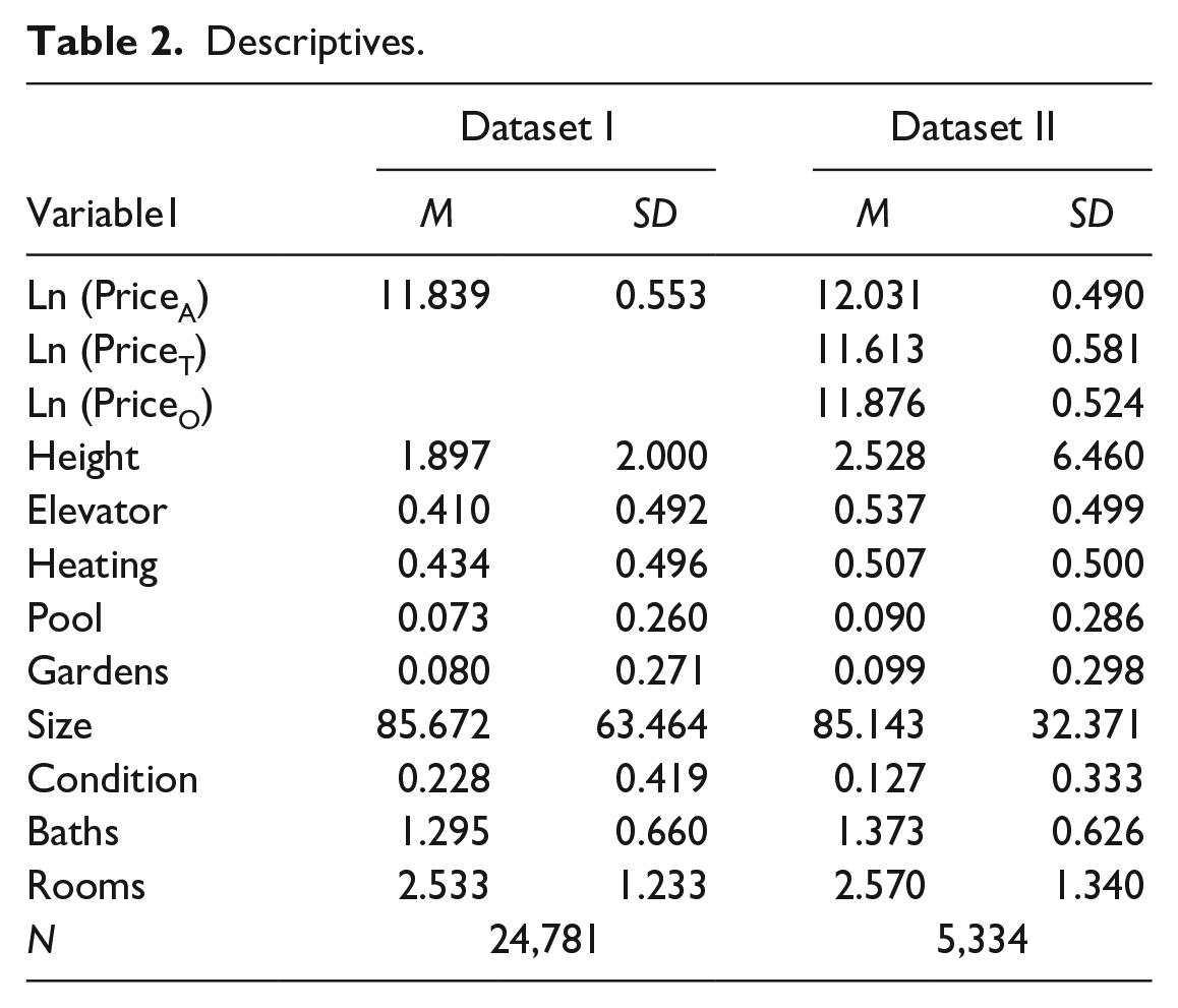
The number of properties analyzed is 24,781. Given that between 2004 and 2013 890,554 housing transactions were conducted (according to the Spanish Ministry of Development), the sample was 2.78% of the complete housing market in Catalonia. 607 postal codes are analyzed in dataset I and 324 in dataset II, which means that the real estates considered are not concentrated and that can be considered as a good sample of the housing market in Catalonia, given that Catalonia comprises 1,146 postal codes. Finally, the period from 2004 to 2013 covers the rise and fall of the Catalan housing market.

All in all, we have created ANN, SLR, and QR models using all the explanatory variables and the appraisal price’s natural logarithm as the variable that needs to be explained. Finally, a combined forecast model has been created by means of WLS regression.

Results and Discussion

Appendix A shows the results for the SLR model. Appendix B shows the QR model results. Appendix C shows the performance of these models. Along with the results for the ANN model.

In regard to the combined model by means of WLS regression, Table 3 shows the results obtained for both variations: with a constant term (Combined 1) and with a suppressed constant term (Combined 2), as well as the performance of the models for dataset I.

Table 3.

Combined Models.

	Combined 1		Combined 2
	Coefficient	t	Coefficient	t
SLR	0.5852	135.09***	0.6167	130.24***
ANN	0.4174	96.46***	0.3834	80.95***
Intercept	−0.0312	−3.07***
R ²	0.7335		0.7356
MAE	0.2146		0.2135
MAPE	0.0183		0.0182
MSE	0.0835		0.0829
RMSE	0.2890		0.2878

***p < .001.

Both combined models perform better than ANN and SLR. In particular, the suppressed constant term model (Combined 2) performs slightly better in line with the findings of Terregrosa and Ibadi (2021). For this reason, we have used the suppressed constant term model (thereinafter WLS) in the forthcoming simulation exercise. WLS model performs also better being applied to dataset II with a R² coefficient equal to .6987 and slightly reducing errors in comparison with SLR (the model with the lowest performance error), namely MAE in 0.0092, MAPE in 0.0008, MSE in 0.0094, and RMSE in 0.0169. Table 4 shows the nonparametric Wilcoxson signed rank test for Dataset II between the absolute forecast errors for the following pairs of models, being all significant: ANN and SLR; ANN and WLS; as well as SLR and WLS.

Table 4.

Wilcoxon Signed Rank Tests.

	SLR-ANN	WLR-ANN	WLS-SLR
Standardized test statistic	13.227	22.837	7.499
Asymptotic significance (two-sided test)	0.000***	0.000***	0.000***

***p < .001.

The effectiveness of the obtained predictions provided by the models has been checked by means of a comparison between the revenues that would be obtained from the property estate sales if these models (ANN, SLR, QR, and WLS) were used to determine the selling price with the actual revenue obtained by the entity. As we will explain later, this simulation exercise has been made for a part of dataset I—only properties with at least one offer have been included—and for the dataset that includes properties that have been sold (dataset II).

Firstly, a model of hedonic prices has been estimated for dataset II. In this model the sale price has been censored (this estimation is available upon request). The reason for censoring is the following: it has been supposed—although not even in this case should be like this, because the price that the purchaser would be ready to pay would be between the price of the last offer and the selling price finally paid—that the price that the purchaser was able to pay is only known if the offer was made before the selling price was determined. Nevertheless, if the property received no offer, the sale price can be considered as the “minimum” price that a purchaser was ready to pay but not as a price that reflects his readiness to purchase it. The prediction of the underlying price in this model is considered the sale price that could have been obtained—and it will be the actual sale price obtained when a sold property has had an offer. For higher prices, it has been considered that the property would have been sold only if the price obtained by any of the procedures would have been lower or equal to the sale price.

Secondly, for the properties in dataset I that had received at least one offer, the lowest price set by the entity is unknown for unsold properties. This lowest price was about 10% and 20% lower than the price published in the web platform where the property was offered. Therefore, a higher price resulting from the analyzed methods would leave the property unsold. Conversely, if the price is lower than the minimum price, the property would be sold. Nonetheless, it has been only considered that the property could have been sold if it had an offer—which value we do not know—and has not been sold. So, if the price provided for each one method is lower than the minimum price and the property had an offer, it is considered that that property could have been sold by the price obtained by that method. This assumption can be considered quite conservative, because properties that have not received any offer may have received them if the minimum price was lower.

With all this information, the percentage of the properties that could have been sold by each of the prices is obtained. And, applying the corresponding price to each of these properties, the total revenues and the revenues per unit sold are arrived at. The method that maximizes total revenues is considered the best one. The total revenues obtained by the properties actually sold is the point of reference. It amounts to €493,366,318. It should be recalled that this price is unknown ex-ante and the purpose is to know by which method we could get closer to it. Finally, the revenues could have been increased in two different ways. First of all, using a different criterion more properties could have been sold. Secondly, more favorable prices could have been obtained in some sales. A Heckman sample selection model has been estimated. The selection parameter (Mills ratio) is not statistically significant. Therefore, it can be inferred that the distribution of sold properties is similar to the properties that have not been sold. The results for ANN, SLR, and QR models are presented in Tables 5 and 6.

Table 5.

Simulation Results.

	Number of sold properties (in percentage)	Total revenues in euros (per property)	Total gross book value in euros (per property)	Total net book value in euros (per property)	Percentage of impairment loss accounted	Capital gain/loss from gross book value in euros (in percentage)	Capital gain/loss from net book value in euros (in percentage)
Sold properties
Actual situation	3,889	493,366,318	807,675,687	591,110,888	26.81	−314,309,369	−97,744,570
Actual situation	(100.00)	(126,862.00)	(207,682.10)	(151,995.60)	26.81	(–38.92)	(–16.54)
ANN	920	174,538,320	211,357,672	157,375,108	25.54	−36,819,352	17,163,212
ANN	(23.66)	(189,715.57)	(229,736.60)	(171,059.90)	25.54	(–17.42)	(10.91)
SLR	952	162,031,296	267,072,842	204,713,130	23.35	−105,041,546	−42,681,834
SLR	(24.48)	(170,200.94)	(280,538.70)	(215,034.80)	23.35	(–39.33)	(–20.85)
QR	1,682	220,109,622	431,427,113	327,595,066	24.07	−211,317,491	−107,485,444
QR	(43.25)	(130,861.84)	(256,496.50)	(194,765.20)	24.07	(–48.98)	(–32.81)
WLS	886	171,839,354	230,553,024	174,936,128	24.12	−58,713,670	−3,096,774
WLS	(22.78)	(193,949.61)	(260,217.86)	(197,444.84)	24.12	(–25.47)	(–1.77)
Total properties	3,889		807,675,687	591,110,888	26.81
Total properties	(100.00)		(207,682.10)	(151,995.60)	26.81
Unsold properties
Actual situation	0	0	0	0	0.00	0	0
Actual situation	(0.00)	(0.00)	(0.00)	(0.00)	0.00	(0.00)	(0.00)
ANN	3,610	545,691,177	409,257,758	380,591,470	7.00	136,433,419	165,099,707
ANN	(40.53)	(151,160.99)	(113,367.80)	(105,427.00)	7.00	(33.34)	(43.38)
SLR	2,429	537,423,264	274,626,141	256,061,294	6.76	262,797,123	281,361,970
SLR	(27.27)	(221,252.89)	(113,061.40)	(105,418.40)	6.76	(95.69)	(109.88)
QR	6,315	540,009,774	674,346,644	614,438,765	8.88	−134,336,870	−74,428,991
QR	(70.89)	(85,512.24)	(106,784.90)	(97,298.30)	8.88	(–19.92)	(–12.11)
WLS	3,487	615,928,302	398,852,475	373,247,434	6.42	217,075,827	242,680,868
WLS	(39.14)	(176,635.59)	(114,382.70)	(107,039.70)	6.42	(54.43)	(65.02)
Total properties	8,908		928,833,597	837,066,053	9.88
Total properties	(100.00)		(104,269.60)	(93,967.90)	9.88
Total properties
Actual situation	3,889	493,366,318	807,675,687	591,110,888	26.81	−314,309,369	−97,744,570
Actual situation	(30.39)	(126,862.00)	(207,682.10)	(151,995.60)	26.81	(–38.92)	(–16.54)
ANN	4,530	720,229,497	620,615,430	537,966,578	13.32	99,614,067	182,262,919
ANN	(35.40)	(158,991.06)	(137,001.20)	(118,756.42)	13.32	(16.05)	(33.88)
SLR	3,381	699,454,560	541,698,983	460,774,423	14.94	157,755,577	238,680,137
SLR	(26.42)	(206,878.01)	(160,218.57)	(136,283.47)	14.94	(29.12)	(51.80)
QR	7,997	760,119,396	1,105,773,757	942,033,831	14.81	−345,654,361	−181,914,435
QR	(62.49)	(95,050.57)	(138,273.57)	(117,798.40)	14.81	(–31.26)	(–19.31)
WLS	4,373	787,767,656	629,405,501	548,183,562	12.90	158,362,155	239,584,094
WLS	(34.17)	(180,143.53)	(143,929.91)	(125,356.41)	12.90	(25.16)	(43.71)
Total properties	12,797		1,736,509,284	1,428,176,942	17.76
Total properties	(100.00)		(135,696.59)	(111,602.48)	17.76

Table 6.

Simulation Results for Total Properties.

	Reversal of impairment losses in euros (in %)	Impairment losses still accounted after the selling in euros (in %)	Combined result
Actual situation	216,564,799	91,767,544	−189,512,114
Actual situation	(70.24)	(29.76)	−189,512,114
ANN	82,648,852	225,683,490	−43,420,571
ANN	(26.81)	(73.19)	−43,420,571
SLR	80,924,560	227,407,782	11,272,354
SLR	(26.25)	(73.75)	11,272,354
QR	163,739,926	144,592,417	−326,506,851
QR	(53.11)	(46.89)	−326,506,851
WLS	81,221,939	227,110,403	12,473,690
WLS	26.34	73.66	12,473,690
Total properties	308,332,342
Total properties	(100.00)

Table 5 shows that, according to the actual situation, 100% of the properties were sold, by a total income of €493,366,318. In the sample of sold properties, the QR was the method that sold the highest percentage (43.25%) of the four compared alternative methods, while the WLS method presents the highest revenues per property. Regarding the sample of the unsold properties it is also the QRs method the one that sells the highest percentage of units (70.89%), while the method that gets the highest revenue per property is the SLR. As a whole, the QR method sells a 62.49% of the sample, hence, it is the method that sells the highest percentage of properties; and the SLR method is the one that obtains the highest revenues per property. Furthermore, the WLS method obtains the highest revenue, followed by the QR, SLR, and the ANN respectively. All the methods analyzed (ANN, SLR, QR, and WLS) obtain higher revenues than in the actual situation. This means that the entity would have earned €266,753,078 more if the QR method had been used. It is true that had the QR method been used, the entity would have fewer assets and according to the criteria of revenues per property, 26% less would have been obtained; but it is also true that with higher sales the bank would have saved many maintenance costs.

On the other hand, the actual situation shows that banks have sold properties with a higher book value than the average of the sample, concretely 53% higher than the gross book value and 36% higher than the net book value. The average value of properties sold by means of the other methodologies is also higher than the average of the sample: 6% more for ANN and QR, 12% more for WLS, and 22% more for SLR from the net book value. Therefore, banks have used, among others, the value of real estates as a criterion to decide which property should be sold, aiming to sell those with a higher book value.

Moreover, the actual situation shows that banks have sold properties whose percentage of impairment loss accounted was particularly high (26.81%) in comparison to both the average of the sample (17.76%) and the properties that have not been sold (9.88%). ANN (13.32%), SLR (19.94%) and QR (14.81%), and WLS (12.90%) models have sold properties whose percentage of impairment loss accounted was slightly inferior to the average of the sample. Hence, a second decision criterion used by banks when deciding which properties would be sold has been the maximization of the reversal of impairment losses. Table 6 shows that €216,567,799 have been reversed from the €308,332,342 of impairment losses that were originally accounted, which represents 70.24%. This is, by far, the highest reversal in comparison with the models analyzed because QR would have only reversed 53.11%, ANN a 26.81%, WLS a 26.34%, and SLR a 26.25% of impairment losses.

Finally, both the actual situation and the QR model have obtained capital losses from the net book value but, on the contrary, ANN, SLR, and WLS models have obtained capital gains. The combined result of capital gains and losses obtained, from the net book value, and the impairment losses not deleted after the selling is shown in Table 6. According to the results obtained, the actual situation is only better than the QR model, ANN model results would still be negative, but SLR and WLS would have provided a positive combined result. Thus, had ANN, SLR, or WLS been used, the financial system would have needed less money or it would have recovered it sooner and, as a result, the Spanish economy would have benefited.

Conclusions

Banks are key agents in the housing market and their economic and financial decisions affect the present and future housing and land use policy. The accumulation of properties by Spanish banks during the crisis is a vivid example of financialization, which has definitely changed the housing market.

In this regard, finding the way to value the properties registered in their balance sheets has been one of the biggest challenges banking industry has dealt with in recent years. There are two advantages in making a good valuation: firstly, the bank’s actual financial situation is known; secondly, properties valued according to the market can be sold more rapidly, which will maximize the revenues obtained (Torres-Pruñonosa et al., 2021). In this paper we aimed to estimate how much the financial entity would have been benefited—by means of an increase of revenues, capital gains generation and the reversal of impairment losses—if those methodologies had been used.

The results suggest that the decision criteria that have been used by banks were selling properties with particularly high book values and percentages of impairment loss accounted. Therefore, banks aimed to maximize the reversal of impairment losses and they achieved it, which provided a better image of their situation in their financial reports. Nonetheless, in comparison with the rest of models, banks did not maximize the selling of properties (only the SLR model sells less properties than the actual situation), obtained the least amount of revenues and obtained the highest capital losses and the second worst combined effect—only the QR model presents a worse combined result. However, the QR method provides another strategic possibility. In this sense, the total revenues and the percentage of properties sold are maximized (only the WLS model obtains higher total revenues). This one would have been the method used if the banking industry wanted to reduce its stock rapidly. The stock would have been halved—about 120,000 units in Spain at the end of 2013—and a huge amount of impairment losses would have been avoided which enhanced the banks’ income statement. Likewise, had this been previously done, the banking bailout would have been avoided partially or, at least, in a lower amount, which would have meant that fewer resources would have been needed in the financial system restructuring.

If banks had used ANN or SLR models, the results obtained would have been much better than the actual situation. Specifically, in comparison with the SLR model, ANN would have sold more properties, generated more revenues, obtained capital gains instead of capital losses and a better combined result than the actual situation, although it would still be negative. On the other hand, in comparison with the ANN model, SLR would have sold less properties, generated less revenues, obtained capital gains and a positive combined result. Finally, had WLS model been used, would have sold more properties than SLR but less than ANN and would have generated the highest amount of revenues, capital gains and combined result. Therefore, this is evidence that the combination of ANN and SLR by means of a WLS regression improves individual models, confirming the findings of Terregrossa and Ibadi (2021). Any of these three methods would have been more efficient than the actual situation. Thus, the financial entities would have maximized results with the beneficial effect that would have transferred to the company, to the shareholders, and even to society, given that a greater percentage of the bailout would have already been paid back. Quite the opposite, banks’ obsession to manipulate accounting by means of maximizing the reversal or impairment losses has been very detrimental to Spanish banking industry and society.

Finally, we would like to point out that the research’s limitation is due to the fact that the amounts of mortgages that use properties as collaterals are currently unknown. Future research will aim to compare the impact of the selection of real estate valuation methods on the risk-weighted assets of banks and, therefore, on their capital ratios.

Footnotes

Appendix

Appendix C.

Performance Measures of the Models Created for Dataset I and II.

Performance measure	Dataset I			Dataset II
Performance measure	SLR	QR	ANN	SLR	QR	ANN
R ²	0.7150	0.5360	0.5835	0.6562	0.2278	0.4934
MAE	0.2159	0.4979	0.2633	0.1721	0.4875	0.3163
MAPE	0.0175	0.0445	0.0224	0.0148	0.0423	0.0274
MSE	0.0853	0.4742	0.1273	0.0663	0.4072	0.1675
RMSE	0.2920	0.6886	0.3568	0.2374	0.5883	0.4092

Declaration of Conflicting Interests

The author(s) declared no potential conflicts of interest with respect to the research, authorship, and/or publication of this article.

Funding

The author(s) disclosed receipt of the following financial support for the research, authorship, and/or publication of this article: We acknowledge support of the publication fee by Universidad Internacional de la Rioja (UNIR), Colegio Universitario de Estudios Financieros, Fundació Tecnocampus Mataró-Maresme and Universidad Rey Juan Carlos.

ORCID iD

Jose Torres-Pruñonosa

References

Aalbers

(2008). The financialization of home and the mortgage market crisis. Competition & Change, 12(2), 148–166.

Akin

Montalvo

García

Peydró

J.-L.

Raya

(2014). The real estate and credit bubble: Evidence from Spain. SERIEs, 5(2), 223–243. https://doi.org/10.1007/s13209-014-0115-9

Alexandridis

K. A.

Karlis

Papastamos

Andritsos

(2018). Real Estate valuation and forecasting in non-homogeneous markets: A case study in Greece during the financial crisis. Journal of the Operational Research Society, 70(10), 1769–1783. https://doi.org/10.1080/01605682.2018.1468864

Ambika

B. J.

Bindush

U. S.

Hemanth

S. D.

(2020). Multi-layer artificial neural network for estimating real-estate prices. International Journal of Advanced Research in Computer Science, 11(1), 105.

Baen

J. S.

Guttery

R. S.

(1997). The coming downsizing of real estate: The implications of technology. Journal of Real Estate Portfolio Management, 3(1), 1–18.

Baldominos

Blanco

Moreno

A. J.

Iturrarte

Bernárdez

Ó.

Afonso

(2018). Identifying real estate opportunities using machine learning. Applied Sciences, 8(11), 2321.

Bartik

T. J.

(1987). The estimation of demand parameters in hedonic price models. The Journal of Political Economy, 95(1), 81–88.

Bates

J. M.

Granger

C. W. J.

(1969). The combination of forecasts. Journal of the Operational Research Society, 20(4), 451–468. https://doi.org/10.1057/jors.1969.103

Bin

(2006). A semiparametric hedonic model for valuing wetlands. Applied Economics Letters, 12(10), 597–601.

10.

Bisello

Antoniucci

Marella

(2020). Measuring the price premium of energy efficiency: A two-step analysis in the Italian housing market. Energy and Buildings, 208, 109670. https://doi.org/10.1016/j.enbuild.2019.109670

11.

Bover

Velilla

(2002). Hedonic house prices without characteristics: The case of new multiunit housing (ECB Working Paper no. 117). https://ssrn.com/abstract=357280

12.

Buchinsky

(1998). Recent advances in quantile regression models: A practical guideline for empirical research. Journal of Human Resources, 33, 88–126, https://doi.org/10.2307/146316.

13.

Buonanno

Montolio

Raya-Vílchez

J. M.

(2013). Housing prices and crime perception. Empirical Econonics, 45, 305–321. https://doi.org/10.1007/s00181-012-0624-y

14.

Byrne

(2020). Generation rent and the financialization of housing: A comparative exploration of the growth of the private rental sector in Ireland, the UK and Spain. Housing Studies, 35(4), 743–765.

15.

Cabrera

Wang

Yang

(2011). Linear and nonlinear predictability of international securitized real estate returns. The Journal of Real Estate Research, 33(4), 565–594.

16.

Chasco

Le Gallo

(2015). Heterogeneity in perceptions of noise and air pollution: A spatial quantile approach on the City of Madrid. Spatial Economic Analysis, 10(3), 317–343. https://doi.org/10.1080/17421772.2015.1062127

17.

Cui

Shen

Feng

(2018). The impact of micro-level influencing factors on home value: A housing price-rent comparison. Sustainability, 10(12), 4343. https://doi.org/10.3390/su10124343

18.

Czembrowski

Łaszkiewicz

Kronenberg

(2016). Bioculturally valuable but not necessarily worth the price: Integrating different dimensions of value of urban green spaces. Urban Forestry & Urban Greening, 20, 89–96. https://doi.org/10.1016/j.ufug.2016.07.010

19.

Cano

F. G.

Etxezarreta

E. A.

Dol

Hoekstra

(2013). From housing bubble to repossessions: Spain compared to other West European countries. Housing Studies, 28(8), 1197–1217.

20.

Çelik

. (2021). The roles of the state in the financialisation of housing in Turkey. Housing Studies.

21.

Chen

C.-L.

Kuan

C.-M.

Lin

C.-C.

(2007). Saving and housing of Taiwanese households: New evidence from quantile regression analyses. Journal of Housing Economics, 16(2), 102–126. https://doi.org/10.1016/j.jhe.2007.01.001

22.

Chiarazzo

Caggiani

Marinelli

Ottomanelli

(2014). A neural network based model for real estate price estimation considering environmental quality of property location. Transportation Research Procedia, 3, 810–817.

23.

Chin

T. L.

Chau

K. W.

(2003). A critical review of literature on the hedonic price model. International Journal for Housing and Its Applications, 27(2), 145–165.

24.

Coq-Huelva

(2013). Urbanisation and financialisation in the context of a rescaling state: The case of Spain. Antipode, 45(5), 1213–1231.

25.

Coulson

N. E.

McMillen

D. P.

(2007). The dynamics of intraurban quantile house price indexes. Urban Studies, 44(8), 1517–1537.

26.

Court

L. M

. (1941). Entrepreneurial and consumer demand theories for commodity spectra. Econometrica, 9, 135–162.

27.

Curry

Morgan

Silver

(2002). Neural networks and non-linear statistical methods: An application to the modelling of price–quality relationships. Computers & Operations Research 29(8), 951–969.

28.

De Ayala

Galarraga

Spadaro

J. V

. (2016). The price of energy efficiency in the Spanish housing market. Energy Policy, 94, 16–24. https://doi.org/10.1016/j.enpol.2016.03.032

29.

A. Q.

Grudnitski

(1992). A neural network approach to residential property appraisal. The Real Estate Appraiser, 58, 38–45.

30.

Grudnitski

(1993). A Neural Network Analysis of the Effect of Age on Housing Values. Journal of Real Estate Research 8(2), 253–264.

31.

Drought

McDonald

(2011). Forecasting house price inflation: A model combination approach [Discussion Paper Series 32]. Reserve Bank of New Zealand.

32.

Duca

J. V.

Muellbauer

Murphy

(2010). Housing markets and the financial crisis of 2007–2009: Lessons for the future. Journal of Financial Stability 6(4), 203–217.

33.

Ebru

Ç.

Eban

. (2009). Determinants of house prices in Istanbul: a quantile regression approach. Quality & Quantity, 45(2), 305–317. https://doi.org/10.1007/s11135-009-9296-x

34.

Ekeland

Heckman

J. J.

Nesheim

(2002). Identifying hedonic models. American Economic Review, 92(2), 304–309.

35.

Ekeland

Heckman

J. J.

Nesheim

(2004). Identification and estimation of hedonic models. Journal of political economy, 112(S1), S60–S109.

36.

Fernández

M. A.

Bucaram

(2019). The changing face of environmental amenities: Heterogeneirty across housing submarketis and time. Land Use Policy, 83, 449–460.

37.

Fernández

Aalbers

M. B.

(2016). Financialization and housing: Between globalization and varieties of capitalism. Competition & Change, 20(2), 71–88

38.

Fernández

Aalbers

M. B.

(2020). Housing financialization in the global south: In search of a comparative framework. Housing Policy Debate, 30(4), 680–701.

39.

Fields

(2017). Unwilling subjects of financialization. International Journal of Urban and Regional Research, 41(4), 588–603.

40.

Follain

J. R.

Malpezzi

(1980). Dissecting housing values and rent. The Urban Institute.

41.

Fuerst

McAllister

Nanda

Wyatt

(2015). Does energy efficiency matter to home-buyers? An investigation of EPC ratings and transaction prices in England. Energy Economics, 48, 145–156. https://doi.org/10.1016/j.eneco.2014.12.012

42.

García

Raya

J. M.

(2011). Price and income elasticities of demand for housing characteristics in the city of Barcelona. Regional Studies, 45(5), 597–608. https://doi.org/10.1080/00343401003713381

43.

García

Raya

J. M.

(2015). Use of a Gini index to examine housing price heterogeneity: A quantile approach. Journal of Housing Economics, 29, 59–71. https://doi.org/10.1016/j.jhe.2015.06.001

44.

Garcia-Lamarca

Kaika

(2016). ‘Mortgaged lives’: The biopolitics of debt and housing financialisation. Transactions of the Institute of British Geographers, 41(3), 313–327

45.

Geng

Bao

Liang

(2015). A study of the effect of a high-speed rail station on spatial variations in housing price based on the hedonic model. Habitat International, 49, 333–339. https://doi.org/10.1016/j.habitatint.2015.06.005

46.

Goodman

A. C.

(1978). Hedonic prices, price indices and housing markets. Journal of urban economics, 5(4), 471–484.

47.

Griliches

(1971). Price indexes and quality change. Harvard University Press.

48.

Gujarati

D. N.

Porter

D. C.

(2010). Econometría (5th ed.). McGraw Hill.

49.

Gupta

Kabundi

Miller

S. M.

(2011). Forecasting the US real house price index: Structural and non-structural models with and without fundamentals. Economic Modelling, 28(4), 2013–2021. https://doi.org/10.1016/j.econmod.2011.04.005

50.

Gutiérrez

Domenech

(2017). The mortgage crisis and evictions in Barcelona: Identifying the determinants of the spatial clustering of foreclosures. European Planning Studies, 26(10), 1939–1960.

51.

Hendel

Nevo

Ortalo-Magné

(2009). The relative performance of real estate marketing platforms: MLS versus FSBOMadison.com. American Economic Review 99(5), 1878–1898.

52.

Hodge

T. R.

McMillen

D. P.

Sands

Skidmore

(2016). Assessment inequity in a declining housing market: The case of detroit. Real Estate Economics, 45(2), 237–258. https://doi.org/10.1111/1540-6229.12126

53.

Hott

(2015). A model of mortgage losses and its applications for macroprudential instruments. Journal of Financial Stability, 16, 183–194.

54.

Jayantha

W. M.

Oladinrin

O. T.

(2019). Bibliometric analysis of hedonic price model using CiteSpace. International Journal of Housing Markets and Analysis, 13(2), 357–371. https://doi.org/10.1108/ijhma-04-2019-0044

55.

Kang

H.-H.

Liu

S.-B.

(2014). The impact of the 2008 financial crisis on housing prices in China and Taiwan: A quantile regression analysis. Economic Modelling, 42, 356–362. https://doi.org/10.1016/j.econmod.2014.07.018

56.

Kang

Lee

H. J.

Jeong

S. H.

Lee

H. S.

K. J.

(2020). Developing a forecasting model for real estate auction prices using artificial intelligence. Sustainability, 12(7), 2899.

57.

Kauko

(2003). On current neural network applications involving spatial modelling of property prices. Journal of Housing and the Built Environment, 18(2), 159–181.

58.

Koenker

Bassett

Jr (1978). Regression quantiles. Econometrica, 1, 33–50.

59.

Lancaster

K. J.

(1966). A new approach to consumer theory. Journal of Political Economy 74(2), 132–157.

60.

Landajo

Bilbao

(2012). Nonparametric neural network modeling of hedonic prices in the housing market. Empirical Economics 42(3), 987–1009.

61.

Lenk

M. M.

Worzala

E. M.

Silva

(1997). High-tech valuation: Should artificial neural networks bypass the human valuer? Journal of Property Valuation and Investment, 15(1), 8–26.

62.

Levitt

S. D.

Syverson

(2008). Market distortions when agents are better informed: The value of information in real estate transactions. The Review of Economics and Statistics, 90(4), 599–611.

63.

Limsombunchai

(2004). House price prediction: Hedonic price model vs. artificial neural network. New Zealand Agricultural and Resource Economics Society, 2014 Conference, June 25–26, Blenheim, New Zealand.

64.

Wei

Y. D.

Tian

(2016). Amenity, accessibility and housing values in metropolitan USA: A study of Salt Lake County, Utah. Cities, 59, 113–125. https://doi.org/10.1016/j.cities.2016.07.001

65.

Wei

Y. D.

Tian

(2019). Analyzing housing prices in Shanghai with open data: Amenity, accessibility and urban structure. Cities, 91, 165–179. https://doi.org/10.1016/j.cities.2018.11.016

66.

Liao

W. C.

Wang

(2012). Hedonic house prices and spatial quantile regression. Journal of Housing Economics, 21(1), 16–27. https://doi.org/10.1016/j.jhe.2011.11.001

67.

Liu

J.-G.

Zhang

X.-L.

W.-P.

(2006). Application of fuzzy neural network for real estate prediction. Advances in Neural Networks (Vol. 3973, pp. 1187–1191), The series Lecture Notes in Computer Science, ISNN 2006. Springer.

68.

McCluskey

W. J.

McCord

Davis

P. T.

Haran

McIlhatton

(2013). Prediction accuracy in mass appraisal: A comparison of modern approaches. Journal of Property Research, 30(4), 239–265.

69.

McCord

M. J.

Davis

P. T.

Bidanset

McCluskey

McCord

Haran

MacIntyre

(2018). House prices and neighbourhood amenities: Beyond the norm? International Journal of Housing Markets and Analysis, 11(2), 263–289. https://doi.org/10.1108/ijhma-04-2017-0043

70.

McGreal

Adair

Mcburney

Patterson

(1998). Neural networks: The prediction of residential values. Journal of Property Valuation and Investment, 16(1), 57–70.

71.

McMillen

D. P.

(2008). Changes in the distribution of house prices over time: Structural characteristics, neighborhood, or coefficients? Journal of Urban Economics, 64(3), 573–589.

72.

McMillen

Shimizu

(2020). Decompositions of house price distributions over time: The rise and fall of Tokyo house prices. Real Estate Economics, 49(4), 1290–1314. https://doi.org/10.1111/1540-6229.12338

73.

McMillen

D. P.

Thorsnes

(2006). Housing renovations and the quantile repeat-sales price index. Real Estate Economics 34(14), 567–584.

74.

Mendelsohn

(1984). Estimating the structural equations of implicit markets and household production functions. The Review of Economics and Statistics 66(4), 673–677.

75.

Migozzi

(2020). Selecting spaces, classifying people: The financialization of housing in the South African City. Housing Policy Debate, 30(4), 640–660.

76.

Mills

E. S.

Simenauer

(1996). New hedonic estimates of regional constant quality house prices. Journal of Urban Economics 2(39), 209–215.

77.

Mora-Garcia

R.-T.

Cespedes-Lopez

M.-F.

Perez-Sanchez

V. R.

Marti

Perez-Sanchez

J.-C.

(2019). Determinants of the price of housing in the Province of Alicante (Spain): Analysis using quantile regression. Sustainability, 11(2), 437. http://dx.doi.org/10.3390/su11020437

78.

Moreno-Izquierdo

Egorova

Peretó Rovira

Más-Ferrando

(2018). Exploring the use of artificial intelligence in price maximisation in the tourism sector: Its application in the case of Airbnb in the Valencian Community. Investigaciones Regionales, 42, 113–218.

79.

Mueller

J. M.

Loomis

J. B.

(2014). Does the estimated impact of wildfires vary with the housing price distribution? A quantile regression approach. Land Use Policy, 41, 121–127. https://doi.org/10.1016/j.landusepol.2014.05.

80.

Nghiep

Cripps

(2001). Predicting housing value: A comparison of multiple regression analysis and artificial neural networks. Journal of Real Estate Research 3(22), 313–336.

81.

Nicodemo

Raya

J. M.

(2012). Change in the distribution of house prices across Spanish cities. Regional Science and Urban Economics, 42(4), 739–748. https://doi.org/10.1016/j.regsciurbeco.2012.05.003

82.

Okkola

Brunelle

(2018). The changing determinants of housing affordability in oil-booming agglomerations: A quantile regression investigation from Canada, 1991–2011. Housing Studies, 33(6), 902–937. https://doi.org/10.1080/02673037.2017.1408784

83.

Owusu-Ansha

(2011). A review of hedonic pricing models in housing research. Journal of International Real Estate and Construction Studies, 1(1), 17–38.

84.

Palmquist

R. B.

(1984). Estimating the demand for the characteristics of housing. The Review of Economics and Statistics 3(66), 394–404.

85.

Palomera

(2014). How did finance capital infiltrate the world of the urban poor? Homeownership and social fragmentation in a Spanish neighborhood. International Journal of Urban and Regional Research, 38(1), 218–235

86.

Park

Bae

J. K.

(2015). Using machine learning algorithms for housing price prediction: The case of Fairfax County, Virginia housing data. Expert Systems with Applications, 42(6), 2928–2934.

87.

Peng

T.-C.

Chiang

Y.-H.

(2015). The non-linearity of hospitals’ proximity on property prices: Experiences from Taipei, Taiwan. Journal of Property Research, 32(4), 341–361. https://doi.org/10.1080/09599916.2015.1089923

88.

Peter

N. J.

Okagbue

H. I.

Obasi

E. C.

Akinola

A. O.

(2020). Review on the application of artificial neural networks in real estate valuation. International Journal of Advanced Trends in Computer Science and Engineering, 9(3), 2918–2925.

89.

Peterson

Flanagan

A. B.

(2009). Neural network hedonic pricing models in mass real estate appraisal. Journal of Real Estate Research, 31(2), 147–164.

90.

Raya

J. M.

Estévez

P. G.

Prado-Román

Torres-Pruñonosa

(2017). Living in a smart city affects the value of a dwelling? In Peris-Ortiz

Bennett

Pérez-Bustamante

Yábar (Eds.), Sustainable smart cities: Innovation, technology, and knowledge management. Springer.

91.

Rolnik

(2013). Late Neoliberalism: The financialization of homeownership and housing rights. International Journal of Urban and Regional Research, 37(3), 1058–1066

92.

Rosen

(1974). Hedonic prices and implicit markets: Product differentiation in pure competition. Journal of Political Economy 1(82), 34–55.

93.

Rossini

P. A.

Kershaw

P. J.

Kooymans

R. R.

(1993). Direct real estate analysis—The upmarket approach to real estate decision making. Third Australasian Real Estate Educators Conference.

94.

Saeidi

Mohammadzadeh

Salmanmahiny

Mirkarimi

S. H.

(2017). Performance evaluation of multiple methods for landscape aesthetic suitability mapping: A comparative study between multi-criteria evaluation, logistic regression and multi-layer perceptron neural network. Land Use Policy, 67, 1–12.

95.

San-José

Retolaza

J. L.

Torres-Pruñonosa

(2020). Eficiencia social en las cajas de ahorro españolas transformadas en bancos. El Trimestre Económico, 87(347), 759–787. https://doi.org/10.20430/ete.v87i347.882

96.

Smart

Lee

(2003). Financialization and the role of real estate in Hong Kong’s regime of accumulation. Economic Geography, 79(2), 153–171.

97.

Selim

(2009). Determinants of house prices in Turkey: Hedonic regression versus artificial neural network. Expert Systems with Applications, 2(36), 2843–2852

98.

Sheppard

(1999). Hedonic analysis of housing markets. In Cheshire

Mills

E. S.

(Eds.), Handbook of regional and urban economics (Vol. 3, pp. 1595–1635). Elsevier.

99.

Tay

D. P.

D. K.

(1992). Artificial intelligence and the mass appraisal of residential apartments. Journal of Property Valuation and Investment, 2(10), 525–540.

100.

Terregrossa

S. J.

(2005). On the efficacy of constraints on the linear combination forecast model. Applied Economics Letters, 12(1), 19–28, https://doi.org/10.1080/1350485042000307062

101.

Terregrossa

S. J.

Ibadi

M. H.

(2021). Combining housing Price forecast generated separately by hedonic and artificial neural network models. Asian Journal of Economics, Business and Accounting, 21(1), 130–148. https://doi.org/10.9734/AJEBA/2021/v21i130345

102.

Timmermann

(2006). Forecast combinations. In Elliott

Granger

C. W. J.

Timmermann

(Eds.), Handbook of Economic Forecasting (Vol. 1, pp. 135–196). Elsevier. https://doi.org/10.1016/s1574-0706(05)01004-9

103.

Tinbergen

(1951). Some remarks on the distribution of labour incomes. International Economic Papers, 1, 195–207.

104.

Torres-Pruñonosa

García-Estévez

Prado-Román

(2021). Artificial neural network, quantile and semi-log regression modelling of mass appraisal in housing. Mathematics, 9(7), 783. https://doi.org/10.3390/math9070783

105.

Trojanek

Gluszak

Tanas

(2018). The effect of urban green spaces on house prices in Warsaw. International Journal of Strategic Property Management, 22(5), 358–371. https://doi.org/10.3846/ijspm.2018.5220

106.

Tuofu

Qingyun

Dongxiao

Xiao

(2021). Evaluating the impact of urban blue space accessibility on housing price: A spatial quantile regression approach applied in Changsha, China. Front in Environmental Science, 9, 696626. https://doi.org/10.3389/fenvs.2021.696626

107.

Wainwright

Manville

(2017). Financialization and the third sector: Innovation in social housing bond markets. Environment and Planning a-Economy and Space, 49(4), 819–838

108.

Wen

Gui

Tian

Xiao

Fang

(2018). Subway opening, traffic accessibility, and housing prices: A quantile hedonic analysis in Hangzhou, China. Sustainability, 10(7), 2254. https://doi.org/10.3390/su10072254

109.

Wen

Xiao

Hui

E. C. M.

(2019). Quantile effect of educational facilities on housing price: Do homebuyers of higher-priced housing pay more for educational resources? Cities, 90, 100–112. https://doi.org/10.1016/j.cities.2019.01.019

110.

Wilhelmsson

Ceccato

(2015). Does burglary affect property prices in a nonmetropolitan municipality? Journal of Rural Studies, 39, 210–218. https://doi.org/10.1016/j.jrurstud.2015.03.01

111.

White

(1988). Economics prediction using neural networks. The case of IBM daily stock return. Neural Networks, IEEE International Conference, 2, 451–459.

112.

Wijburg

Aalbers

M. B.

(2017). The alternative financialization of the German housing market. Housing Studies, 32(7), 968–989.

113.

Worzala

Lenk

Silva

(1995). An exploration of neural networks and its application to real estate valuation. Journal of Real Estate Research, 10(2), 185–201.

114.

Luo

(2017). Spatial effects of accessibility to parks on housing prices in Shenzhen, China. Habitat International, 63, 45–54. https://doi.org/10.1016/j.habitatint.2017.03.010

115.

Yang

Chu

Gou

Yang

Huang

(2020). Accessibility and proximity effects of bus rapid transit on housing prices: Heterogeneity across price quantiles and space. Journal of Transport Geography, 88, 102850. https://doi.org/10.1016/j.jtrangeo.2020.102850

116.

Zahirovich-Herbert

Gibler

K. M.

(2014). The effect of new residential construction on housing prices. Journal of Housing Economics, 26, 1–18. https://doi.org/10.1016/j.jhe.2014.06.003

117.

Zhang

(2018). What contributes to the rising house prices in Beijing? A decomposition approach. Journal of Housing Economics, 41(C), 72–84. https://doi.org/10.1016/j.jhe.2018.04.003

118.

Zietz

E. N.

Sirmans

G. S.

(2007). Determinants of house prices: A quantile regression approach. The Journal of Real Estate Finance and Economics, 37(4), 317–333. https://doi.org/10.1007/s11146-007-9053-7

119.

Zwan

(2014). Making sense of financialization. Socio-Economic Review, 12(1) 99–129.

How on Earth Did Spanish Banking Sell the Housing Stock?

Abstract

Keywords

Introduction

The Spanish Case

Methodology

Results and Discussion

Conclusions

Footnotes

Appendix

Declaration of Conflicting Interests

Funding

ORCID iD

References