Sage Journals: Discover world-class research

Abstract

In this study, we analyze the probability of bank failure, the expected losses, and the costs of bank restructuring with the application of a lognormal distribution probability function for three categories of European banks, that is, small, medium, and large, over the post-crisis period from 2012 to 2016. Our goal was to determine whether the total capital ratio (TCR) properly reflects banks’ solvency under stress conditions. We identified a phenomenon that one can call the “crooked smile of TCR”. Medium-sized banks with relatively high TCRs performed poorly in stress tests; however, the probability of bank failure increases slightly with the size of the bank, while the TCR decreases. We claim that the focus on capital adequacy measures is not sufficient to achieve the goal of improving banks’ stability and reducing their restructuring costs. Our results are of special importance for medium-sized banks, as these banks are not regularly subjected to publicly available stress tests.

Keywords

bank failure restructuring costs stress tests total capital ratio

Introduction

The global financial crisis (GFC), which erupted in 2007 to 2008, caused European taxpayers to provide banks with extensive financial assistance to avoid significant market disturbances and a loss of trust among bank customers. The large amounts of money used to recapitalize banks stimulated a discussion about the cost of bank restructuring and the possible steps to be taken to reduce the probability of future crises and to reduce their costs. The first wave of measures included more restrictive regulations on banks’ capital adequacy and liquidity (called Basel 3), which were supposed to fill the regulatory gaps identified after the outbreak of the GFC. The second wave of the measures introduced within the reforms included a resolution regime, which was first used during the savings and loans (S&L) crisis in the US in the 1980s. The idea of a resolution consists of a bank’s orderly liquidation to avoid market disturbances and the use of taxpayer money for a bank bailout. Dewatripont and Freixas (2011) presented a resolution as a compromise between financial stability and economic activity. Small banks are expected to undergo a regular bankruptcy procedure, while medium-sized and large banks may undergo a resolution procedure. According to the EU regulations provided in the Bank Resolution and Restructuring Directive (BRRD, 2014/59/EU), under certain restrictive conditions, in addition to the resolution procedure, precautionary recapitalization is allowed, but this tool is supposed to be used only for large banks with systemic importance. Under the BRRD framework, unlike the cases of its initial use, a bail-in is included. A bail-in, as opposed to a bailout, requires covering losses from bank capital and eligible liabilities (i.e., those that are allowed to be subject to a bail-in according to the law). As Benink (2018) noticed, the credibility of the bail-in mechanism is rather limited due to an insufficient level of debt that may be subject to a bail-in. Thus, banks need to keep relatively high capital buffers. Briefly, capital buffers are the difference between the total capital ratio (TCR) and the threshold of 8% set by the Basel Committee on Banking Supervision. Nevertheless, the first line of defense to cover losses is bank capital; therefore, the capital ratio remains the crucial measure to evaluate banks’ capacity to cover losses. From a policy-making perspective, it is important to link the level of capital ratios with the costs of bank restructuring or failure.

The goal of this study is to analyze whether the TCR properly reflects banks’ solvency under a stress scenario and to estimate the cost of banks’ failure against this background. To this aim, we analyze the probability of bank failure, expected losses and, finally, the costs of bank restructuring with the application of a lognormal distribution probability function for three groups of banks categorized according to size. Our analysis indicates that it is not always the case that the TCR reflects banks’ solvency under a stress scenario. To assess banks’ ability to recover from high losses, one should also rely on a stress-testing analysis of risk-generating assets, which is reflected in this study by the novel beta ( $β$ ) coefficient. The results suggest that some banks with a relatively high TCR perform poorly in stress tests. Our main contribution to the literature is the evaluation of the TCR’s importance under stressed conditions for different groups of banks, while most previous studies did not account for bank heterogeneity. Moreover, the results of our study may help policy makers set up benchmark capital ratios for banks of different sizes to maximize their resilience and reduce the cost of failures.

The remainder of the paper is organized as follows. Section 2 presents a review of the literature and develops research hypotheses. In section 3, we explain the data sources and the methodology, while in section 4, we discuss the empirical results. The last section concludes.

Literature review

The literature on financial stability, bank risk, and crisis prevention is abundant and rapidly expanding. Therefore, we focus on the two strands of the literature most related to the main topic of our investigation, namely, (1) capital ratios and—on their background—the cost of bank restructuring and (2) stress tests used to detect banks’ financial problems.

The literature indicates that the cost of bank resolution is conditional on the mechanisms and economic conditions under which bank distress occurs. From a theoretical perspective, Gaffeo and Molinari (2015), by using a network model, compared liquidations and bail-ins as restructuring alternatives. For insolvency-driven defaults, the fire sales of assets (as a consequence of bail-ins) cause contagion, which can be reduced by higher capital. Therefore, because of the Basel 3 reform, the externalities and the potential for contagion should decline. Capponi et al. (2017) evaluated two types of policies designed to control systemic risk, specifically, capital requirements and mitigation policies applied in the case of bank default. The authors found that the conservation and countercyclical capital buffers introduced by Basel 3 reduce the number of defaults and the average loss per default. Moreover, within the purchase and assumption process, auctioning a bank in smaller pieces reduces deposit insurance institutions’ losses. Similarly, Leanza et al. (2021), in their analysis of bail-ins versus bailouts, concluded that tighter capital requirements implemented under the Basel 3 framework can be effective in “taming leverage and default risk.” In the same vein, Stopczyński (2020) postulated that capital buffers should remain high to retain banks’ loss absorption capacity.

As noted by Schnabel (2020), the use of bail-in tools is often regarded as “highly political and controversial,” even in times of no systemic crisis. This remark was made after an analysis of resolution practices under a single resolution mechanism (SRM) in the euro area. Therefore, the role of capital ratios is crucial to facilitate resolution.

Iwanicz-Drozdowska et al. (2016) found that the rescue operations in the EU during the GFC were the most expensive (per bank) in the case of medium-sized banks, while for small banks, the cost was slightly higher than the cost for large and systemically important banks. Bennett and Unal (2014) claimed that the cost of resolution tools critically depends on the macroeconomic context. The authors showed that private sector solutions (i.e., purchase and assumption) lead to a higher loss on assets and are costlier than simple liquidation. However, the loss on assets is lower for private sector reorganizations when the industry is not in distress. The findings presented by Bennett and Unal (2014) correspond well with the phenomenon identified by Cowan and Salotti (2015) who established that regulators subsidize healthy banks to purchase failed banks during a crisis. The authors showed that the stockholders of acquiring banks captured significant positive capital adequacy ratios. An additional cross-sectional analysis revealed that these gains included significant wealth transfer that resulted from the regulatory acceptance of bids below the failed banks’ fair value.

As a positive role of capital ratios (including buffers) and the importance of bank capital for the cost of restructuring are emphasized in the literature, we suggest the first research hypothesis (H1) as follows: a high bank capital ratio (TCR) allows to minimize the costs of bank restructuring.

The second strand of the literature, which is important from the perspective of our research goal, pertains to stress tests. Stress tests started to gain in popularity after the outbreak of the GFC to evaluate banks’ resilience. From this time on, supervisors conducted regular stress tests, and the results were publicly available. Additionally, banks conduct their own stress tests that are not available to the public. The literature does not agree on whether stress tests provide new information for interested parties. On the one hand, Quijano (2014), with regard to the bond market, and Morgan et al. (2014), with regard to the stock market, maintained that stress tests reveal previously unknown information. On the other hand, Lazzari et al. (2017) showed that the comprehensive assessment performed by the European Central Bank in 2014 did not add much to the publicly available information and provided limited assistance to the market in discriminating between good and bad banks. These authors claimed that the outcomes of the comprehensive assessment (including stress tests) were valuable mainly because they predicted the supervisory policy stance and its severity. Moreover, Schuermann (2020) indicated that supervisors should not use one stress test scenario but a wider range of scenarios with the inclusion of nonfinancial risks to avoid “model monoculture.” These nonfinancial risks are becoming important, for example, climate risk.

Despite the ambiguous evidence concerning the relevance of stress tests, numerous researchers have attempted to identify weaknesses in the current approaches and have proposed new techniques that are better adapted to heterogeneous banking organizations. Wu et al. (2018) underscored that the main challenge in stress testing is model instability. Using data on auto loans, the authors showed that the coefficients of macroeconomic variables vary substantially across different sample periods, which, in turn, casts doubt on the reliability of stress test results. Cerutti and Schmieder (2014) argued that stress tests based on consolidated data may underestimate the capital needs of large, geographically diversified banks because they disregard ring fencing-type behaviors by regulators during financial crises. Model and data risks boost efforts to elaborate the validation methods for bank stress test models (Kupiec, 2018).

The development of stress test techniques is rapid. However, none of the new models have yet emerged as a clear winner. New approaches to bank stress testing encompass a concentration on rare risk events that can result in crises in banking systems (Hu et al., 2014) or the exploitation of different artificial intelligence/machine learning solutions (Climent et al., 2019; Gogas et al., 2018). For example, Kolari et al. (2019), using the AdaBoost approach, confronted this methodology with the results of the European Banking Authority (EBA) stress test in 2010, 2011, and 2014. It was possible to identify 98% of the “failing” and “passing” banks in the training sample and 90% in the test validation sample. The authors concluded that passing the stress test depended on the financial condition (profitability and impaired loans) and the macroeconomic environment (unemployment rate and public debt) of individual banks but not on the severity of the stress test scenario. Therefore, even lenient stress tests may improve the assessment of the failure risk.

A separate group of studies on bank stress testing has underlined the merits of accounting for banks’ heterogeneity. Kapinos and Mitnik (2016) applied the top-down stress testing approach to US banks to show the resilience of individual banks and the banking sector to macroeconomic shocks. The authors’ dependent variable was the ratio of equity to total assets (leverage), and their goal was to predict the level of leverage after any shock, on the bank and industry levels. The authors found that considering the heterogeneity of banks significantly changes the estimates of expected capital shortfalls. Busch et al. (2018) developed a stress test model especially designed for small and medium-sized banks, which are usually ignored under standard approaches. The authors combined a credit risk stress test with an income stress test. The elaboration of specific stress test techniques designed for smaller banking organizations is also justified by the work of DeYoung et al. (2018) who showed that small banks react differently than large banks to capital shocks.

As stress tests allow us to evaluate banks’ resilience to crisis events, we suggest the second research hypothesis (H2) as follows: stress tests are a helpful subsidiary tool to evaluate banks’ restructuring costs.

Moreover, Walther and White (2020) suggest that regulators should have a mandate to take action on publicly available information, not on regulators’ private information, to reduce “zombie lending” by banks that are undercapitalized. This is a tool of a disciplinary nature for regulators and policy makers to avoid pressure for bailouts. However, only the results of certain stress tests are publicly available, while most constitute a type of “private information.”

Against this background, our study attempts to expand the scope of the analysis of European banks by combining the costs of restructuring and stress tests. The inspiration for our analysis is the fact that regulatory measures, such as the total capital ratio, are not free from limitations, although they have been modified within the post-crisis regulatory overhaul. Therefore, as already presented in several studies, stress tests constitute a good complementary tool to detect bank problems to react in advance. Reasonable levels of capital ratios complemented by resolution tools should enable the reduction of the costs of bank restructuring.

Data and Methodology

We use empirical data for European banks (EU countries and Switzerland due to their uniform accounting standards) from the Orbis Bank Focus for the post-crisis period that ranges from 2012 to 2016. We choose the post-crisis period because the new regulatory solutions that were implemented initiated a new era in banking. The observations vary in their completeness, that is, for many banks, just some of the possible figures are reported. After rejecting incomplete observations, 4,719 small bank, 1,410 medium-sized bank, and 508 large bank observations are taken into account.

We divide banks into the following three groups based on their total assets: ‘small’ banks with assets lower than EUR 3 billion; “medium” banks with assets between EUR 3 billion and EUR 30 billion; and “large” banks with assets exceeding EUR 30 billion. This aims to capture the different effects that originate from the size of banks. When facing financial difficulties, small and medium banks can undergo bankruptcy, whereas large banks used to be “bailed out” by governments to avoid a disastrous impact on local and global financial systems (this was a typical practice before the introduction of the Bank Recovery and Resolution Directive, BRRD). The EUR 3 billion and EUR 30 billion thresholds are chosen based on the following criteria:

banks with balance sheet totals up to EUR 3 billion are treated in European Commission documents related to state aid as small banks; and

banks with balance sheet totals over EUR 30 billion are often called “too-big-to-fail,” which is motivated by the threshold defined in Article 4 (10) (a) of the Bank Recovery and Resolution Directive (BRRD).

Bailout criteria are expected to be restrictive to reduce moral hazard (e.g., Freixas & Rochet, 2013; Gong & Jones, 2013). Due to more restrictive capital regulations, by including capital buffers for global and domestic systemically important banks (G-SIBs and D-SIBs), we assume that once large banks encounter financial problems, they will meet the criteria for precautionary recapitalization specified in the BRRD and will thus not be in a “critical” situation.

Taking into account balance sheet structures, we divide banks’ assets into two parts, namely, assets that are risk-free and assets that are risk-generating. We take two different approaches toward the definition of risk-free assets. First, based on the assumption that sovereign exposures do not bear risk, risk-free assets are the sum of cash and debt securities issued by governments. In the second approach, we additionally assume that bank bankruptcies are rare, and we thus include loans provided to other banks. The differences between these two approaches prove to be insignificant; therefore, we present in detail only the results of the first approach (the authors can share the results of the second approach on request).

The following high-level balance sheet structure is analyzed:

A_{r f} + A_{n r f} = D + L_{b a i l i n} + C A P

(1)

where $A_{r f}$ are the risk-free assets, $A_{n r f}$ are the risk-generating assets, $D$ are customer deposits covered by the deposit guarantee system, $L_{b a i l i n}$ are liabilities that may be subject to a bail-in (which we assume to be the difference between total liabilities and $D$ ), and $C A P$ refers to bank capital (tier 1 and tier 2). Our balance-sheet equation is similar to Stopczyński (2020) and Leanza et al. (2021). However, in contrast to Leanza et al. (2021), we do not separate the covered bonds that are not eligible for a bail-in, and we do not use the charter value on the asset side. Neither study differentiates assets according to their risk, while our study differentiates assets according to their risk. The analysis is performed by using the share of each balance sheet item in the balance sheet total.

The guaranteed deposit level is computed with the use of the country-specific cut-off (CF) rates indicated by Cannas et al. (2015) as follows (please see Annex 1):

D = C F \cdot D E P

(2)

where DEP represents the total sum of the customer deposits.

Below, we provide concise descriptive statistics of the sample. The histograms of the most important variables are provided in Figure 1 for the small (S) banks, in Figure 2 for the medium (SL) banks, and in Figure 3 for the large (L) banks. The respective information on the minimum/maximum value, average, median, and standard deviation are presented in Table 5.

Figure 1.

Histograms of the most important variables in the small bank group.

Figure 2.

Histograms of the most important variables in the medium bank group.

Figure 3.

Histograms of the most important variables in the large bank group.

A visual inspection of the histograms together with a brief analysis of the figures yield the following insights.

Total assets ( $A_{r f} + A_{n r f})$ . For all three groups of banks, the distribution of total assets is skewed—the observations are concentrated close to the lower limit of the interval. This skewness is most profound for the large banks for which more than 50% of the observations lie below 100 billion EUR. However, this is expected, because in this category, there is no upper limit defined (recall that a large bank is defined to have more than 30 billion EUR on the balance sheet).

Tier 1 and Tier 2 capital (CAP). It seems that capital is the least skewed variable (the most evenly distributed around its mean value). The small banks exhibit the highest capital ratio, and the large banks exhibit the lowest capital ratio. However, the capital of the small banks is the most dispersed (it has the highest standard deviation), while it is the least dispersed for the large banks. These effects can be explained by the ability of asset diversification and capital optimization, which is positively correlated with the total asset level.

Non-risk-free assets ( $A_{n r f})$ . Non-risk-free assets are considerably high for all three bank groups, and they are the highest for small banks and the lowest for large banks. The distribution of non-risk-free assets is very skewed and is concentrated at approximately 85% to 90% with a tail to the left side of the mean. This pattern underlines that the small banks hold relatively smaller amounts of cash and government securities and are to a larger extent focused on loans to customers.

Guaranteed deposits (D). Customer deposits under the guarantee system have quite different distributions among the bank groups. Although they exhibit similar shapes for the small and medium banks (a concentration of approximately 55% and a longer tail to the left), this cannot be said for the large banks, where the distribution is somewhat uniform. The histograms also show that when a bank is larger, more observations lie closer to 0%. We assume that this is because the balance sheets of the small and medium banks are more “standard,” with a strong retail customer base, while the larger banks may have more specialized profiles, such as wholesale or SMEs.

Liabilities subject to bail-in ( $L_{b a i l i n})$ . Perhaps the most interesting variable in the dataset are the liabilities that can be used for a bail-in and cover the losses. Similar to guaranteed deposits, the shape of this distribution is similar for the small and medium banks (which is concentrated at approximately 40% with a longer tail to the right), while it is more uniform for the large banks. It is interesting to see that the mean L_bailin is nearly twice as small for the small banks as for the large banks (and for the medium banks, it lies in between). We believe that this is because the small banks exhibit a higher percentage of capital and are more retail customer-driven (and therefore have more deposits under the guarantee scheme), which means that fewer liabilities can be used in the case of a “fail.”

We identify the loss events as the reporting events in which the after-tax profit is negative. The probability of loss, which is determined as the share of the loss events in all reported events for each group separately, is presented in Table 1. The figures are based on Orbis Bank Focus data.

Table 1.

The Frequency of Loss $p_{l o s s}$ for the Three Groups of Banks.

Small banks	4.81%
Medium banks	7.54%
Large banks	14.87%

Note. Based on data from Orbis Bank Focus.

When looking at the differences among the three groups, the first conclusion is that the larger banks face losses more frequently than the smaller banks, as shown in Table 1. However, the reported losses for the small banks are on average higher and more dispersed (i.e., the standard deviation is higher) than the losses for the medium and large banks (see Table 2). This might indicate that larger banks can allow for more frequent loss, but their capability of hedging and managing the risk allows for reducing the relative scale of loss (i.e., a fraction of the balance sheet total or assets).

Table 2.

Loss Empirical Distribution Characteristics for the Three Groups of Banks.

Size	Mean (%)	Median (%)	Min (%)	Max (%)	St. dev. (%)	Ex. kurtosis
Small	2.2	1.0	0.005	41	3.7	52.0
Medium	2.0	0.9	0.001	14	2.9	4.5
Large	1.5	0.7	0.001	13	2.1	11.9

Note. Based on data from Orbis Bank Focus.

We assess the loss distribution based on two assumptions, specifically,

• It is one-sided (loss is always negative) and

• It is heavy-tailed (because we model bank failures, which have a very low probability but a very high financial impact).

Another observation that originates from the empirical loss distribution statistics (presented in Table 2) is that the excess kurtosis (which is the difference between the kurtosis of the sample and the kurtosis of the Gaussian distribution) is always positive and very high for the small banks compared to the medium and large banks. This result confirms our assumption that the distribution of losses is “heavy-tailed.”

As no natural candidate distribution is found in this case, the first candidate for fitting is the generalized extreme value (GEV) distribution, which covers the most common heavy-tailed distributions. The GEV distribution is a three-parameter family of continuous distributions introduced by Jenkinson (1955) with regard to assessing the frequency distribution of the annual maxima of meteorological events. Over the years, the distribution became increasingly popular when modeling rare and extreme events in various disciplines and industries. Such a GEV fit was compared with less general distributions, such as Fréchet and lognormal and generalized Pareto distributions. The sensitivity analysis shows that the results of the GEV distribution cannot be fully comparable with the results of the other candidates. The three alternative distributions are commonly used for fitting heavy-tailed datasets. All distributions yield very similar results for the small and large banks, while for the medium banks, the Fréchet distribution provides somewhat smaller expected losses. As the Fréchet distribution has a less realistic fit close to zero in all cases and the generalized Pareto and lognormal distributions give very close results to one another, we choose the lognormal distribution for further analysis. All results based on the Fréchet or generalized Pareto distributions are available on request.

The lognormal distribution has the following functional form:

\begin{array}{l} F_{a, b, c} (x) = \frac{c}{a} y^{c - 1} e x p (- y^{c}), \\ w h e r e y = \frac{x - b}{a}, x > 0, c > 0 . \end{array}

(3)

In equation (3), $F_{a, b, c}$ is the cumulative distribution function of the lognormal distribution, and $a, b$ , and $c$ are its parameters, where a determines the scale, b determines the location, and c determines the shape. The parameters of the fit are presented in Table 3, and the fitted lognormal distributions are presented in Figure 4.

Table 3.

The Parameters of the Lognormal Fit to Losses Incurred by the Banks From the Three Bank Groups.

Parameter	Small banks	Medium banks	Large banks
a	0	0	0
b	0.011	0.007	0.006
c	1.28	1.56	1.45

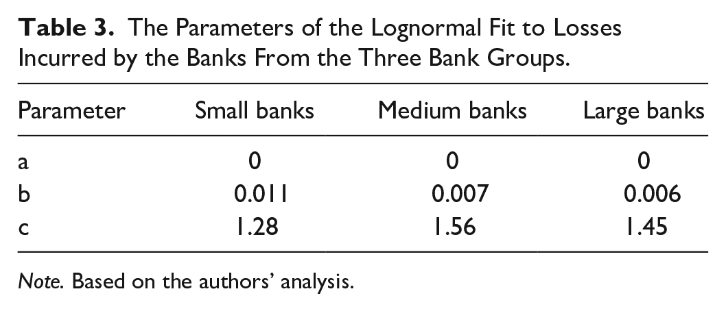
Note. Based on the authors’ analysis.

Figure 4.

The lognormal distributions fitted to the empirical loss distributions for the three bank groups.

The fitted distributions presented in Table 3 and illustrated in Figure 4 show quantitative differences in the loss distributions of the three bank groups. More specifically, as seen in Table 4, the distribution mean for the small banks is comparable with the mean for the medium banks, whereas the mean for the large banks is the lowest. Thus, on average and based on the lognormal distribution, the small and medium banks incur higher losses than the large banks compared with their total assets.

Table 4.

Statistical Means of the Three Lognormal Distributions.

Measure	Small banks	Medium banks	Large banks
Mean	0.023	0.025	0.018

Note. Based on the authors’ analysis.

Based on the results of research by Philippon and Salord (2017) who argue that two-thirds of the recapitalization is covered by governments and one-third represents the loss of owners and creditors, we say that a bank “fails” when the loss exceeds 33% of the bank’s capital. This choice might be considered to be quite arbitrary. For this reason, an additional sensitivity analysis was performed that shows that the results are quite stable in a $\pm 3$ p.p. interval around this value.

According to the three fitted lognormal distributions $p (x)$ , we calculate the “probability of failure” in the following way.

1. For the small and medium banks, the probability of loss times the probability that the loss will be greater than 0.33 of the bank’s capital. We assume that the loss of 0.33 CAP will very likely result in bank insolvency because smaller banks may not be capable of attracting new investors to increase bank capital. Such a loss depletes a significant part of tier 1 capital, and the bank will not be allowed to operate in the market due to capital constraints; it may undergo restructuring with the use of, for instance, a forced merger or acquisition, or it may be declared bankrupt. The “probability of fail” may thus be expressed as

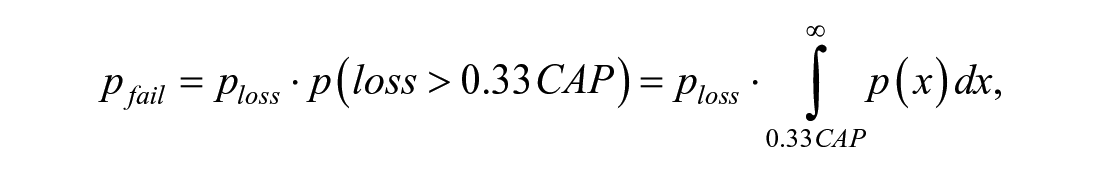
p_{f a i l} = p_{l o s s} \cdot p (l o s s > 0.33 C A P) = p_{l o s s} \cdot \int_{0.33 C A P}^{\infty} p (x) d x,

where for simplicity reasons, the relevant lognormal probability density is expressed as $p (x)$ .

2. For the large banks, the loss times the probability that the loss will be between 0.33 CAP and CAP. We assume that the large banks exhibit adequate capacity to attract new capital and that a loss below one-third of their capital will not cause failure; however, a higher loss requires intervention and recapitalization or resolution measures. We also assume that the loss will not exceed the amount of Tier 1 and Tier 2 capital because large banks are supposed to have high capital cushions to absorb losses. These banks are not expected to declare bankruptcy due to their systemic importance. In this case, the “probability of fail” may be expressed as

\begin{array}{l} p_{f a i l} = p_{l o s s} \cdot p (0.33 C A P < l o s s < C A P) \\ = p_{l o s s} \cdot \int_{0.33 C A P}^{C A P} p (x) d x . \end{array}

Based on the above, we calculate the expected loss that results from the “fail” as the expected value (based on the lognormal distributions $p (x)$ ) of the loss under the condition that it is greater than 0.33 CAP for the small and medium banks or as the expected value of the loss under the condition that it is between 0.33 CAP and CAP for the large banks. This is mathematically expressed in the following way:

\begin{array}{l} E x p (l o s s) = \frac{\int_{0.33 C A P}^{\infty} x \cdot p (x) d x}{\int_{0.33 C A P}^{\infty} p (x) d x} \\ f o r t h e s m a l l a n d m e d i u m b a n k s a n d \\ E x p (l o s s) = \frac{\int_{0.33 C A P}^{C A P} x \cdot p (x) d x}{\int_{0.33 C A P}^{C A P} p (x) d x} f o r t h e b i g b a n k s . \end{array}

To estimate the cost of bank restructuring, we introduce the beta coefficient, which is the ratio of risk-generating assets after the failure to the risk-generating assets before the failure, that is,

β = \frac{A_{n r f} - E x p (l o s s)}{A_{n r f}}

(4)

This equation shows how much is left out of the initial value of bank risk-generating assets after the probability of failure materialized, and this parameter is important from the restructuring cost perspective.

The full cost of bank restructuring can now be estimated. For the small banks, the cost is assumed to be the minimum of

(1) $C A P + L_{b a i l i n}$ (a higher value would have to be covered by the guaranteed deposits, which is beyond the scope of this analysis due to bankruptcy rules),

(2) the non-risk-free assets (which cannot be outbalanced by the loss), or

(3) the expected loss.

For the medium banks, if the mean loss is greater than $C A P + L_{b a i l i n}$ or $A_{n r f}$ , then it is beyond the scope of the resolution, that is, the bank fails. We reject such results in this analysis. In other cases, the full cost of restructuring is assumed to be the following:

(1) if $E x p (l o s s) < C A P$ , then twice the expected loss (the bank loses assets and then recapitalizes to the previous level of capital); or

(2) if $C A P < E x p (l o s s) \leq C A P + L_{b a i l i n}$ , then the sum of the capital and the expected loss (the bank uses all of its capital and recapitalizes the loss from the bail-in liabilities up to the level of Exp(loss)).

The large banks’ recapitalization cost is assumed to be twice the expected loss; that is, the loss depletes the bank capital, and then, it is recapitalized to the previous CAP level.

Results and discussion

In Table 5, the results of the analysis are reported for the three bank groups. The loss statistics are presented in Table 2. In general, the mean and median losses are quite small compared to the modeled expected loss for all three groups of banks, as shown in Tables 2 and 5. This result is not surprising; the expected loss is calculated under the condition of the bank’s failure, which is an extreme event.

Table 5.

Statistics for the Three Bank Groups.

Small banks	Min.	Max.	Average	Median	St. dev.
Total assets*	9	2,998	823	572	728
TCR* (%)	0.4	95.9	18.8	17.7	6.2
CAP* (%)	0.0	82.7	10.8	10.3	4.1
A_nrf* (%)	11.3	100.0	92.8	96.0	9.5
L_bailin* (%)	10.6	97.8	38.9	37.5	8.8
D* (%)	0.0	80.5	50.3	51.6	9.0
Prob. of fail** (%)	0.0	4.8	0.9	0.9	0.3
Beta** (%)	44.5	97.6	90.4	91.0	2.9
Exp. loss** (%)	2.4	45.0	8.7	8.6	2.2
Full cost** (%)	2.4	45.0	8.8	8.6	2.2
Medium banks	Min.	Max.	Average	Median	St. dev.
Total assets*	3,007	29,971	9,180	6,865	6,373
TCR* (%)	4.8	93.3	18.1	16.5	7.4
CAP* (%)	0.0	43.6	8.9	8.6	3.9
A_nrf* (%)	40.4	99.9	88.4	92.1	10.6
L_bailin* (%)	7.4	97.1	47.5	43.1	15.6
D* (%)	0.0	76.5	43.5	48.4	15.4
Prob. of fail** (%)	0.2	7.5	1.6	1.5	0.6
Beta** (%)	60.5	97.3	88.4	89.1	3.8
Exp. loss** (%)	2.6	32.3	10.0	9.9	2.7
Full cost** (%)	2.6	64.5	18.8	18.5	6.1
Large banks	Min.	Max.	Average	Median	St. dev.
Total assets*	30,009	2,164,103	267,108	93,758	409,448
TCR* (%)	0.9	87.5	18.2	16.4	9.5
CAP* (%)	0.0	29.6	6.2	5.6	3.2
A_nrf* (%)	19.7	99.5	87.4	88.9	9.8
L_bailin* (%)	32.8	97.3	64.6	62.8	16.4
D* (%)	0.0	61.4	29.3	31.0	15.7
Prob. of fail** (%)	0.0	4.3	2.4	2.3	0.8
Beta** (%)	84.0	100.0	96.0	96.4	2.0
Exp. loss** (%)	0.0	15.3	3.4	3.1	1.7
Full cost** (%)	0.0	30.6	6.8	6.3	3.3

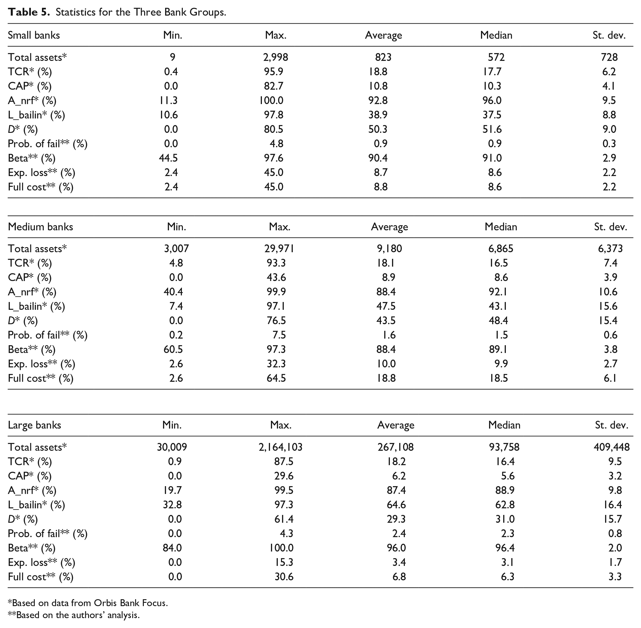
Based on data from Orbis Bank Focus.

Based on the authors’ analysis.

Based on the results of our analysis, which accounts for the heterogeneity of banks as in for example, Kapinos and Mitnik (2016), presented in Table 5, the small banks exhibit the highest TCR and CAP (the bank capital to assets ratio), which is supported by the lowest probability of failing, while their beta, expected loss, and full cost are intermediate between those of the medium and large banks (similar to e.g., Capponi et al., 2017; DeYoung et al., 2018; Leanza et al., 2021). In the case of the large banks, one observes the highest probability of failure and beta and the lowest capital ratios, expected losses and full cost. This result shows the financial strength of large banks because even in the case of a loss event, they do not face a significant drop in the value of their assets (which is reflected as 1 − $β$ ). Such results may be explained by a better diversification of their assets and activities and higher expertise in risk management.

Although the small banks are expected to have less diversified (or highly concentrated) assets and represent lower risk management expertise, their restructuring costs are at a medium level, while for the medium banks, the loss in the value of assets (1 − $β$ ) and the full cost of restructuring are the highest. The beta coefficient for the medium banks also shows the highest variance (second power of standard deviation) among all three groups. This indicates that the loss of the value of assets is difficult to predict for the medium banks (as the variance of the beta coefficient is the highest), whereas it is more concentrated around the average for the small and large banks. We conjecture that this might be related to the fact that medium-sized banks enter new business areas to gain market share and increase profitability, but as they do not represent such good expertise in risk management, they have to face losses more frequently than large banks. In contrast to medium banks, small banks stick to their regular and traditional business areas, which they know very well and thus face less severe losses.

Consistent with these findings, we suggest that a proper combination of capital ratios and risk expertise allows banks to reduce the costs of restructuring. For small banks, a business focus and strong capital ratios seem to be the key, while for large banks, better risk expertise, more diversified activities, and slightly lower capital ratios enable them to reach the lowest costs of restructuring. Medium-sized banks, since they do not manage to gain sufficient risk expertise but instead strive to expand, suffer losses the most. Moreover, the largest banks are more frequently scrutinized by supervisors, as they are of systemic importance and—if listed on the stock exchange—they are disciplined by the market.

Since the implementation of Basel 1 in 1988, bank supervisors have directed special attention to the bank solvency ratio (currently referred to as the TCR). The common understanding is that when the TCR is higher, the bank is safer. Table 5 contains the TCR statistics for the three bank groups. As the average values are similar, the standard deviation is higher for the medium banks than for the small banks and highest for the large banks. Figure 5 also shows that indeed, for the small banks, when the TCR is higher, the probability of “fail” is lower; however, this relation is diminished somewhat for the medium banks and is hardly apparent for the largest banks. This, in turn, suggests that when a bank is larger, it provides less TCR information. This conclusion may be explained by the higher capability of medium and large banks to reduce the TCR level, which is again due to the application of more advanced methods, that is, based on internal models, to calculate this ratio. Small banks usually do not use advanced approaches for this purpose.

Figure 5.

TCR plotted against the probability of “fail” for the three bank groups.

Moreover, our analysis further suggests that the TCR cannot be treated as an absolute figure. For example, which can also be observed in Figure 5, for a TCR between 19% and 21% (this interval has been chosen for the following example, and the conclusion does not change for other similar intervals), the maximum probability of “fail” equals 2.9% for small banks, 4.1% for medium banks, and 3.9% for the largest banks. A similar result is observed for the average probability of “fail” in this interval, which is equal to 0.8% for small banks, 1.5% for medium banks, and 2.2% for large banks. This again suggests that the TCR is more restrictive for small banks, whereas medium and large banks can have similar levels of the TCR while exhibiting a higher probability of “fail.”

Figure 6 supports the traditional understanding of the TCR. It illustrates the trends (by a trend here, we mean a moving average of 50 observations) of the TCR and the probability of “fail,” which is plotted against the logarithm of total assets. The probability of “failure” grows slightly with total assets, while the TCR decreases. This means that when a bank is more likely to fail, it has a lower TCR. The visible dependence between the TCR and the probability of “fail” on total assets is worth noting here. This dependence is not very strong, however, as we only see it on the logarithmic scale.

Figure 6.

Logarithmic moving average of the TCR and the probability of “fail” versus total assets. A window of 50 observations was taken as the moving average.

Figure 7 shows a comparison of the full failure cost versus the TCR for all three bank groups. To interpret the results, one must start by observing that the full cost of a “fail” event does not reflect the probability of such an event. The construction of the analysis relies on random losses that are higher than CAP (0.33 CAP for large banks). When CAP is higher, the probability of “failure” is lower, and the cost of potential “failure” is higher. 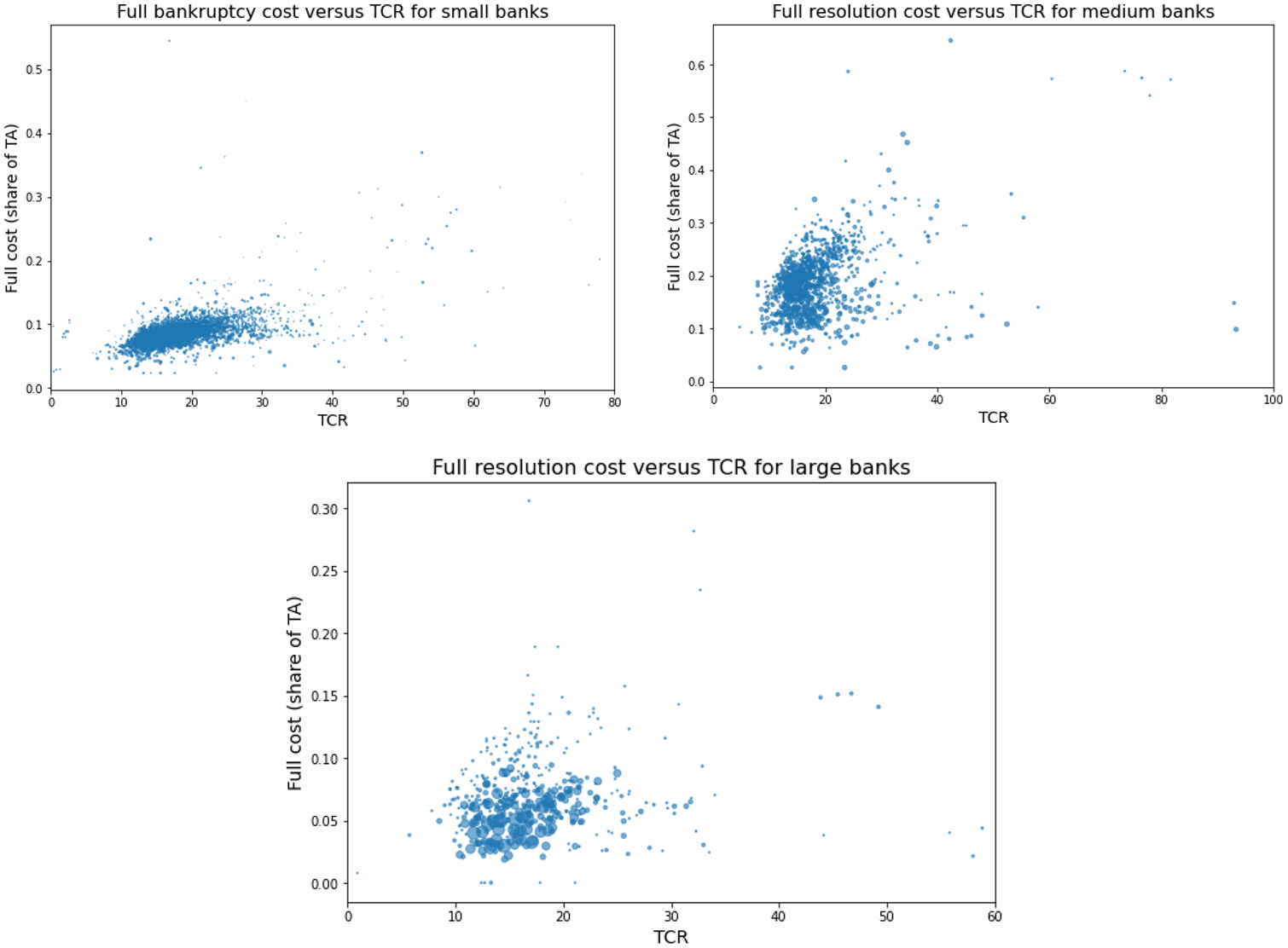A simple linear regression, $F u l l_c o s t = a \cdot T C R$ , can help determine how strongly the full cost of a “fail” event rises with the TCR level. The results show that the a parameter is considerably lower for the small and large banks than for the medium banks. This suggests that for the same TCR, the expected cost of “fail” is considerably higher for the medium banks than for the other types of banks. This is another argument for not a full “applicability” of the TCR to banks with high total assets.

Figure 7.

TCR plotted against the full cost of “fail” for the three bank groups.

What are the practical implications of “the crooked smile of TCR?” First, supervisors may use this type of analysis to set a benchmark TCR for banks of different sizes to minimize the probability of their failure and to reduce the cost of their restructuring. This may allow them to adjust the capital buffers for different groups of banks. Supervisors have access to information on banks’ loan portfolio structure; therefore, they could determine corporate default risk shocks to account for the vulnerabilities of different industries (e.g., COVID-19 crisis in Aiyar et al., 2021) to estimate the level of $β$ . Estimations based on such data are expected to be more accurate.

Second, we postulate that various stakeholders should not limit their analysis to basic capital ratios but rather should look at the structure of banks’ assets, especially risk-generating assets and their concentration. These findings are in line with for example, Kapinos and Mitnik (2016), DeYoung et al. (2018), and Schuermann (2020). An analysis of the decrease in the value of assets (proxied by 1 $- β$ ) should be the focus. Therefore, the stress testing of assets is of special importance and should be regularly conducted for small banks (e.g., Busch et al., 2018), albeit in a very simplified way focused on credit risk concentration. To avoid imposing an additional burden on small banks, institutional protection schemes (developed for cooperative banks) and supervisors should be responsible for the stress test. For medium-sized banks, these stress tests should either be simplified if they focus only on traditional business or similar to the advanced stress tests for large banks if they enter non-traditional business areas.

We claim that capital ratios should be interpreted as adequate only in conjunction with asset stress test results. Not all stakeholders have access to individual bank stress test results. Regarding supervisory practices, there are three types of stress tests, namely, aggregated stress tests, which do not present information on individual banks, individual bank stress tests, which are conducted by using scenarios provided by supervisors and are disclosed to the public (e.g., EBA stress tests), and individual bank stress tests, which are conducted with the use of bank scenarios and are not disclosed to the public (internal use only with confidential information provided to the supervisor). The first two types of stress tests often focus on large, systemically important banks. The reliability of the results of these tests is strongly based on the quality of the stress test scenario provided by the regulator. Because their results are disclosed to the public, the scenarios are quite often moderate rather than severe. These results are treated as a reassuring confirmation that the banking sector and individual banks are safe and sound. If any stakeholders use this type of stress test as a complementary tool, then they will improve their knowledge about bank risk exposure to a certain extent but not completely. Small and medium-sized banks are commonly not covered by this type of stress test. Moreover, individual and confidential bank stress tests are potentially the best source of complementary information but are not available to the public. However, it is necessary to emphasize that the reliability of this stress test is also influenced by the quality of the stress test scenario. To obtain a genuine picture, the stress test scenario should be severe to correctly reflect the risk of extreme events. The content of the scenario depends on the management board’s decisions. If management prefers to obtain a reassuring confirmation of their risk management policy, then the scenario will be moderate in the toughest version. Therefore, regulators should devote special attention to the scenario’s severity. We suggest including this assessment as a part of an incentive system for bank management. If the stress test scenario is evaluated as reliable, then it will have a positive impact on the bonus. Otherwise, the scenario will be treated as a malus for bank management. Without such stimuli, managers will be inclined to apply nonsevere scenarios.

Conclusions and Policy Implications

The goal of our study was to analyze whether the TCR properly reflects bank solvency under a stress scenario and to estimate the cost of bank failure. We investigated the probability of failure, the expected loss and the full cost of bank restructuring for European banks divided into the three groups of small, medium, and large banks over the post-crisis period of 2012 to 2016. The choice of the probability distribution has a moderate effect on the results. Four distributions were considered, specifically, a GEV distribution, Fréchet distribution, generalized Pareto distribution, and lognormal distribution. Of these four, all but the GEV distribution yielded comparable results, and the generalized Pareto and lognormal distributions were the most similar.

The main conclusion of our analysis is that analysts should not put all their trust in the TCR, particularly for medium-sized banks, as it might not be a good indicator of the bank’s possible failure cost. Our findings did not provide support for H1. We argue that capital buffers combined with reasonable risk expertise and traditional business are sufficiently fair to reduce the ex-ante restructuring costs for small banks. In this case, stress tests may be of a supportive nature, especially to detect excessive concentration risk. For the largest banks that represent the highest risk expertise, capital buffers and stress tests alongside supervisory scrutiny are sufficient tools to minimize restructuring costs.

As confirmed in this study, the focus on capital adequacy measures, such as the TCR, is not sufficient to achieve the goals of improving the stability of banks and reducing their restructuring costs. This is especially the case for medium-sized banks, for which a stress test of the value of their assets should complement typical regulatory measures. Our results provide support for H2 since $β$ (which shows a drop in the value of assets) differs among the three bank groups and reflects their vulnerability to risk. It is especially important for medium-sized banks for which restructuring costs were the highest. This is because they may expand their activities in the various business areas in which they do not have good expertise and, therefore, suffer higher losses than the other types of banks. The use of stress test results is advisable, however, for all groups. Moreover, we suggest that the stress test scenarios accepted by boards of management should be severe to show the most reliable picture of a bank’s financial position. An assessment of the reliability of these scenarios conducted by supervisory authorities must become a component of incentive systems for bank management bodies.

The phenomenon of “the crooked smile of TCR” was pronounced in the case of medium-sized banks, and consequently, this result strongly suggests the inadequacy of the standard procedures aimed at assessing medium-sized banks’ solvency. Therefore, we postulate treating stress test results as a subsidiary part of banks’ capital adequacy assessment. Stress tests should be focused on the loss in the value of assets scenario, which—with the use of more granular data and industry information available to supervisors—may provide accurate results regarding banks’ resilience. The simulations based on aggregated data may not provide satisfactory results.

Moreover, our findings support the changes envisaged by the approaching Basel 4 regulations, which consist of reducing the options for more advanced calculations of capital requirements and should make the TCR more comparable in the future. As a result, the link between the level of the TCR and the probability of failure will be clearer for banks of all sizes. The coming quarters and years should also reveal the effectiveness of the post-GFC regulatory reform, as banks are currently undergoing a real-time stress test due to the SARS-CoV-2 pandemic.

Our work is not free from limitations. First, based on the data granularity and a high number of missing values in the Orbis database, a quite high-level balance sheet structure was assumed. It would be preferable to model more subtle balance sheet movements, for example, to replicate the ways that banks optimize the TCR, or to use direct data on guaranteed deposits.

The second limitation is a moderately low number of observations for large banks. Based on 511 observations, it is, of course, possible to perform a statistical analysis; however, this comes at the cost of all distributions being less “smooth” (see Figure 3), and a couple of large outliers could possibly affect the results. We did not identify such outliers, however.

Footnotes

Annex 1

We use the following cut-off rates proposed by Cannas et al. (2015): (CF): CF = 0.85 if COUNTRY = “DK” OR “SI”; CF = 0.61 if COUNTRY = “EE” OR “FI”; CF = 0.72 if COUNTRY = “FR” OR “ES” OR “AT”; CF = 0.75 if COUNTRY = “GR”; CF = 0.78 if COUNTRY = “NL”; CF = 0.57 if COUNTRY = “IE”; CF = 0.67 if COUNTRY = “LT” OR “PT” OR “BE”; CF = 0.19 if COUNTRY = “LU”; CF = 0.41 if COUNTRY = “LV”; CF = 0.74 if COUNTRY = “MT”; CF = 0.67 if COUNTRY = “DE” OR “CH” OR “HR” OR “CY” OR “CZ”; CF = 0.59 if COUNTRY = “PL”; CF = 0.83 if COUNTRY = “RU”; CF = 0.90 if COUNTRY = “SK”; CF = 0.71 if COUNTRY = “SE”; CF = 0.70 if COUNTRY = “BG”; CF = 0.69 if COUNTRY = “HU”; CF = 0.56 if COUNTRY = “UK”; and CF = 0.68 if COUNTRY = “IT.” We assume the same rates for Switzerland and Germany.

Declaration of Conflicting Interests

The author(s) declared no potential conflicts of interest with respect to the research, authorship, and/or publication of this article.

Funding

The author(s) disclosed receipt of the following financial support for the research, authorship, and/or publication of this article: This article is based on a research grant (KZiF/S/19/18) conducted in 2018 in the Management and Finance Collegium at Warsaw School of Economics (Poland).

ORCID iD

Małgorzata Iwanicz-Drozdowska

References

Aiyar

Dao

M. C.

Jobst

Mineshima

Mitra

Pradhan

(2021). COVID-19: How will European Banks fare? IMF.

Benink

H. A.

(2018). Raising bank loss absorption capacity through equity capital or bail-in debt: A perspective from Europe. Journal of Financial Economic Policy, 10(2), 275–280.

Bennett

R. L.

Unal

(2014). The effects of resolution methods and industry stress on the loss on assets from bank failures. Journal of Financial Stability, 15, 18–31.

Busch

Koziol

Mitrovic

(2018). Many a little makes a mickle: Stress testing small and medium-sized German banks. The Quarterly Review of Economics and Finance, 68, 237–253.

Cannas

Cariboni

Kazemi Veisari

Pagano

(2015). Updated estimates of EU eligible and covered deposits. JCR Technical Report (doi: 10.2788/44868)

Capponi

Dooley

J. M.

Oet

M. V.

Ong

S. J.

(2017). Capital and resolution policies: The US interbank market. Journal of Financial Stability, 30, 229–239.

Cerrutti

Schmieder

(2014). Ring fencing and consolidated banks’ stress test. Journal of Financial Stability, 10, 1–12.

Climent

Momparler

Carmona

(2019). Anticipating bank distress in the Eurozone: An extreme gradient boosting approach. Journal of Business Research, 101, 885–896.

Cowan

A. R.

Salotti

(2015). The resolution of failed banks during the crisis: Acquirer performance and FDIC guarantees, 2008–2013. Journal of Banking & Finance, 54, 222–238.

10.

Dewatripont

Freixas

(2011). Bank resolution: A framework for the assessment of regulatory intervention. Oxford Review of Economic Policy, 27(3), 411–436.

11.

DeYoung

Distinguin

Tarazi

(2018). The joint regulation of bank liquidity and bank capital. Journal of Financial Intermediation, 34, 32–46.

12.

Freixas

Rochet

J. C.

(2013). Taming systemically important financial institutions. Journal of Money Credit and Banking, 45(Suppl. 1), 37–58.

13.

Gaffeo

Molinari

(2015). Interbank contagion and resolution procedures: Inspecting the mechanism. Quantitative Finance, 15(4), 637–652.

14.

Gogas

Papadimitriou

Agrapetidou

(2018). Forecasting bank failures and stress testing: A machine learning approach. International Journal of Forecasting, 34, 440–455.

15.

Gong

Jones

K. D.

(2013). Bailouts, monitoring, and penalties: An integrated framework of government policies to manage the too-big-to-fail problem. International Review of Finance, 13(3), 299–325.

16.

Yan

Zhao

J. L.

Hua

(2014). Ontology-based scenario modeling and analysis for bank stress testing. Decision Support Systems, 63, 81–94.

17.

Iwanicz-Drozdowska

Smaga

Witkowski

(2016). Bank restructuring in the EU. Which way to go? Journal of Policy Modeling, 38(3), 572–586.

18.

Jenkinson

A. F.

(1955). The frequency distribution of the annual maximum (or minimum) values of meteorological elements. Quarterly Journal of the Royal Meteorological Society, 81, 158–171.

19.

Kapinos

Mitnik

O. A.

(2016). A top-down approach to stress-testing banks. Journal of Financial Services Research, 49(2–3), 229–264.

20.

Kolari

J. W.

López-Iturriaga

F. J.

Sanz

I. P.

(2019). Predicting European bank stress tests: Survival of the fittest. Global Finance Journal, 39, 44–57.

21.

Kupiec

P. H.

(2018). On the accuracy of alternative approaches for calibrating bank stress test models. Journal of Financial Stability, 38, 132–146.

22.

Lazzari

Vena

Venegoni

(2017). Stress tests and asset quality reviews of banks: A policy announcement tool. Journal of Financial Stability, 32, 86–98.

23.

Leanza

Sbuelz

Tarelli

(2021). Bail-in vs bail-out: Bank resolution and liability structure. International Review of Financial Analysis, 73, 101642.

24.

Morgan

D. P.

Peristiani

Savino

(2014). The information value of the stress test. Journal of Money Credit and Banking, 46, 1479–1500.

25.

Philippon

Salord

(2017). Bail-ins and bank resolution in Europe: A progress report, Geneva reports on the world economy (4th special report). CEPR.

26.

Quijano

(2014). Information asymmetry in US banks and the 2009 bank stress test. Economics Letters, 123, 203–205.

27.

Schnabel

(2020). Are banks finally resolvable? A perspective from Europe. Journal of Money Credit and Banking, 52(S1), 77–86.

28.

Schuermann

(2020). Capital adequacy pre- and postcrisis and the role of stress testing. Journal of Money Credit and Banking, 52(S1), 87–105.

29.

Stopczyński

A. R.

(2020). Estimating the required amount of a bank’s loss-absorbing capacity. Emerging Markets Finance and Trade. Advance online publication. https://doi.org/10.1080/1540496x.2020.1810012

30.

Walther

White

(2020). Rules versus discretion in bank resolution. Review of Financial Studies, 33(12), 5594–5629.

31.

Fang

Wang

(2018). An empirical study of bank stress testing for auto loans. Journal of Financial Stability, 39, 79–89.

“The Crooked Smile of TCR”: Banks’ Solvency and Restructuring Costs in the European Banking Industry