
Abstract
This study claims to be the first in assessing the short-run and long-run impacts of both the size and composition of fiscal adjustment on the growth in Pakistan. Empirical calibration has been made on Mankiw et al.’s model, while the Autoregressive Distributed Lag (ARDL) techniques of Pesaran et al. have been employed to carry out the estimation. To cure the problem of degenerate cases, the ARDL techniques have been augmented with the model of Sam et al. The analysis supports the hypothesis of “expansionary fiscal contraction” in the long run. The analysis reveals that the spending-based adjustment enhances the economic growth, whereas the tax-based adjustment would reduce the growth in the long run in the case of Pakistan. The Granger causality test indicates that the fiscal adjustments have been weakly exogenous, thereby allowing feedback effect from the economic growth toward the fiscal adjustment. Thus, the objective of sustained economic growth can be achieved through the spending-based consolidation measures.
Introduction
The employment of fiscal policy to the ultimate goal of economic development is a controversial issue (Organisation for Economic Co-Operation and Development [OECD], 2008). There are many factors that determine economic growth; however, it seems rather complex to disentangle the growth impact of fiscal policy and determine the causal loops with certainty. Often policy makers are clear about the strategy of interventions in the economy. Sometimes, though, they are left baffled and confused by the rapid changing world scenarios as like the rest of us. Among the strategies of intervention, fiscal actions have been extensively directed to promote growth. But the success story of such interventions is, however, limited to the developed world. Today it is more obvious that imprudent fiscal interventions work like a double-edged sword: The current generation gets benefits at the expense of the future generation.
Economists normally measure the success of a government in terms of its ability to raise enough revenue and such revenue is expected to be utilized for current operations of the government and even in projects which promote future growth. However, such ability depends on the taxation structure and even on the efficient spending strategy of a country. Such fiscal interventions may have both direct and indirect effects on the welfare of the current and future generations. Developing countries often fail to mobilize their domestic resources efficiently as compared with the developed ones. This failure is partly attributed to low tax base, larger proportion of agriculture sector in gross domestic product (GDP), institutional problems including corruption in tax administration, and tax exemptions, and partly to imprudent spending strategy. But the question is why fiscal policy could not deliver in developing countries and what makes them unable to mobilize domestic resources efficiently and adopt effective spending strategy. The answer to this question may lie in poor information of the fiscal managers regarding the optimal fiscal stance stemming from underdeveloped research on the pace of changing world scenarios.
Like other developing countries, Pakistan has been confronted with the enigma of fiscal deficits due to the increasing interference in economic affairs. Today, persistent fiscal deficit is believed to have some serious consequences for the economy; it exacerbates balance of payment deficit, leads to financial instability, crowds out private investments, undermines a country’s international credit worthiness, accelerates inflation, and reduces competitiveness in the world market. Resultantly, fiscal deficit has not only attracted the attention of policy makers and politicians but often becomes talk of the town. Similarly, developing countries are more conscious about the issue of fiscal deficit and consider it the main cause of other macroeconomic imbalances in the economy (Zaidi, 2005).
Since 1990, Pakistan’s economy did not experience a smooth pattern of economic growth. During this period, the economy suffered from inconsistent growth trajectory with occasional surges in economic growth tracked by economic recessions. Besides this, the country is facing the problem of twin deficits, which has resulted in mounting public debt liabilities. Consequently, debt servicing consumes a large portion of the federal budget in the face of depleted foreign exchange reserves in the country. Moreover, recent macroeconomic imbalances are being associated with the structural bottlenecks in the economy, which have largely been ignored for decades on the pace of insufficient policy responses.
Official statistics indicate that over the past 5 years, Pakistan has achieved a moderate average growth rate of 4.7% against the 5.4% target. During this period, economic growth has largely remained consumption oriented. Fiscal deficits over the years have resulted from the unplanned and unproductive public expenditures with low growth in revenues, while low exports and high imports led to deficit in current accounts. Against a pensive target of 6.2%, the economy grew at a meager speed of 3.29% in FY 2018–2019. The saving-investment gap during the same period remained as 4.7% of the GDP. Total investment was recorded as 15.4%, while national savings stood at 10.7% of the GDP. Further official statistics reveal that the average fiscal deficit remained 5.6% of GDP over the past 5 years: with average expenditures stood at 20.5% against average revenue reached to 14.9% of GDP. The average inflation on the basis of Consumer Price Index (CPI) over the last 5 years remained 4.8% with 7% during July–April (2018–2019), while deficit on the current account stood at 6.3% of the GDP in 2017–2018 amounting to US$19.9 billion (Economic Survey of Pakistan [ESP], 2018–2019). Looking at the tax structure over the past three decades, it is pertinent to indicate that Pakistan is facing dramatic shifts in its revenue structure and is on the move from indirect to direct taxation. Similarly, political instability, inconsistent macroeconomic policies, floods, and internal insurgency did not leave the fiscal space for rainy days, and therefore the need for further research over the issue at hand increases.
In response to the recent fiscal imbalance dialogue and the resulting macroeconomic issues, this article endeavors to investigate some important questions such as: What is fiscal adjustment (FA)? When will it succeed? And how does it affect the economic growth? More importantly, the objective is two-pronged. First, the periods of FA have to be identified to isolate the true fiscal stance; second, attempt will be made to quantify the growth impact of the FAs in the case of Pakistan. To achieve the objective, the empirical model will be calibrated on the famous growth model of Mankiw et al. (1992). To estimate the model, Pesaran et al.’s (2001) Autoregressive Distributed Lag (ARDL) techniques will be employed. Furthermore, to cure the problem of degenerate cases, the ARDL techniques would be augmented with the Sam et al. (2019) techniques.
Exploring answers to these questions, while employing ARDL techniques, is expected to add some important insights into the empirical literature across the world in general and Pakistan in particular. Such empirical insights, complemented by the dynamic analysis, would be helpful in identifying the optimal fiscal actions with respect to timing, size, and policy mix in Pakistan. Therefore, efforts shall be devoted to such analyses which necessarily simplify the issues surrounding the practical policy options in a developing country like Pakistan.
Review of Literature
Several theoretical approaches have been evolved that guide the empirical investigation in isolating the macroeconomic effects of fiscal policy. However, among these, three approaches regarding the effectiveness of fiscal policy have emerged. These include the Keynesian, the Neo-classical, and the Ricardian equivalence hypothesis (REH). The Keynesian approach, under the assumption of price rigidity, predicts a multiplier effect of expansionary fiscal policy on the output and employment, and terms it the “Crowding-In” effect. Contrary to this, the Neo-classical approach negates such a multiplier effect. This approach recognizes the “Crowding-Out” effect and argues that the expansionary fiscal actions will crowd out private investments when a government comes in competition with the private sector in the loan market thereby increases interest rates. Such a multiplier effect is likely to be more dampened when the private investments remain more interest-sensitive. The REH, on the other extreme, negates both the Keynesian and the Neo-classical, and argues no impact of fiscal policy. The multiplier effect under the Keynesian approach is based on their analysis of the demand side of the economy. But others focus on the supply-side impacts that may influence the multiplier effect (Choi & Devereux, 2006). According to Keynesian approach, macroeconomic imbalances are mainly caused by excess or deficient aggregate demand as compared with aggregate supply, and therefore rely on the demand-side tools. The demand-side tools are further divided into two categories. The first is known as built-in-stabilizer, while the second is referred to as discretionary fiscal instruments. It is therefore necessary to explain and distinguish these concepts from each other.
Theoretically, the fiscal policy consists of two components: the endogenous movement of the fiscal variables over the business cycles and discretionary fiscal actions by the government. The first component is termed as built-in-stabilizer, while the latter is coined as discretionary fiscal stance. Further investigation reveals that two components of the discretionary fiscal policy have extensively debated in the discipline of public finance. Of these, the first component is found to be exclusively dependent on the macroeconomic environment of the economy, while the second is not influenced by such environment of the economy. The second component is composed of the discretionary fiscal actions that are normally implemented for political gains or in the pursuit of the ruling party’s ideology (Fatas & Mihov, 2003).
It is a common phenomenon that public spending and taxes vary over time. Such variations can be attributed to the automatic movement of spending and taxes during business cycles (i.e., boom and recession) and partly due to the discretionary policy actions, for instance, tax rate changes. Business cycles, which are the recurrent ups and downs in aggregate economic activities, extended over a period of time normally result in government expenditures and tax revenue changes. This tendency of public spending and tax revenues to move over the business cycles is called automatic or built-in-stabilizers, and is capable to partly control the fluctuations of the economy both in the periods of recession and boom. In the absence of any active fiscal actions, the transfer payments usually fall during the boom time with a simultaneous increase in tax collections imposed on consumption, corporation, and labor incomes. The opposite will happen during the recessionary period.
The supply-side approach which is based on Real Business Cycle (RBC) theory rejects the demand-side fiscal instruments and connotes that supply-side expansion will foster economic growth (Cuestas & Ordóñez, 2018). Since Neo-classical assumes flexible prices, they therefore argue that expansionary fiscal policy would reduce private investments, and thereby undermines growth prospects. Unlike Keynesian, this approach considers aggregate supply as the main determining factor of output in the economy stemming from the change in the marginal tax rate. Such a change in this rate will change the relative price of work against leisure and the opportunity cost of consumption against savings and investment. Consequently, the supply of output will be encouraged in the economy when the marginal tax rate falls and would be discouraged when the marginal tax rate rises. However, individuals would attempt to smooth their consumption over fluctuations in their incomes. Under the RBC model, such behavior is quietly capable to minimize the crowding-out effect of expansionary fiscal actions. When the government increases its expenditures, then individuals start expecting tax burden in the future, and they, therefore, increase their supply of labor to smoothen their consumption over time. Other factors that would affect the supply-side stimulus include the labor supply elasticity and the degree of intertemporal consumption. Besides this, the crowding-out effect will be further offset if the government’s investments complement rather than substitute the private sector investments (Cuestas & Ordóñez, 2018). Woodford (2011) argues that RBC model would envisage a positive response of output if firms increase their production in response to increasing aggregate demand. This production effect will be stronger if monetary policy is accommodative under the assumption of sticky prices.
In response to the Great Depression, the writings of Keynes in the form of the General Theory of Employment, Interest, and Money provide a solid foundation to fiscal policy for the role it plays in stabilizing the aggregate economic activities. In this regard, the prime achievement of Keynes is the re-establishment of the notion about the ineffectiveness of the fiscal policy in influencing the aggregate economic activities (Blinder & Solow, 1973). Before Keynes, tools of fiscal policy were mainly used to redistribute and channelize resources from households and business firms to public sector and had no role to bring stability in the economic fluctuations. After Keynes, expansionary fiscal policy has been considered as helpful in reducing the fluctuations in aggregate demand when the economy operates below its potential level of output (Vladimirov & Neicheva, 2008). Furthermore, the Keynesian’s view advocates countercyclical fiscal policy to minimize output gap via restoring equilibrium in the labor market (Burda & Wyplosz, 1997).
At the other extreme, the Neo-classical models argue that fiscal consolidation will stimulate economic activities in the short run and ensure sustainability of public finances of a country in the long run (Vladimirov & Neicheva, 2008). However, a number of factors have been identified that influence the short-run effects of the FA. Such factors include the types of taxation, elasticity of labor supply, and size and persistence of the discretionary fiscal impulse (Baxter & King, 1993). An interesting debate on the short-run impacts of fiscal consolidation can be found in the study of Palley (2013). In addition, this view emphasizes on the possibility of tax distortion effect on the expenditure multiplier and can make it negative in the short run as opposed to the conventional IS-LM model (Vladimirov & Neicheva, 2008). Theoretically, such negative relationship between government expenditures and output stems via three channels: the wealth effect, tax distortion, and intertemporal substitution (Baxter & King, 1993; Perotti, 1999). Contrary to the conventional IS-LM model, the wealth effect through a Ricardian channel emerges as long as people start expecting future tax burden. This will reduce the present value of the household’s income arising from the current fiscal expansion (Vladimirov & Neicheva, 2008). As a result, the supply of labor increases thereby enhancing the marginal productivity of the capital and stimulates investments in a country (Burnside et al., 2004). Furthermore, the persistence of the fiscal expansion is expected to determine the size of wealth effect and such effect would be stronger when the expansion becomes more persistent (Choi & Devereux, 2006).
While Keynesian and Neo-classical approaches disagree on the macroeconomic effects of the fiscal policy, Barro (1989) postulates REH. In a study, Barro (1990) assessed REH by analyzing the impact of the fiscal balance on private investment and growth. He took 98 countries over the sample period from 1960 to 1985. The study finds no direct connection between the public deficit and economic productivity, and arrives at the conclusion that rather than spending on general welfare programs and subsidies provision to agriculture sector, economic growth is likely to be positively influenced by infrastructure development. However, one should remember that REH is based on certain strong assumptions, such as perfect foresight, time horizon, full liquidity constraints, perfect capital market, and altruistic desire of the current generation not to pass on fiscal burden to the future generation. Such assumptions do not normally meet, and thereby justify the relationship between the fiscal actions and private consumption (Blanchard, 1985; Mankiw & Summers, 1984). Based on such strong assumptions, REH practically becomes insignificant at least in its perfect form (Hemming et al., 2002). Fiscal policy can thus retain its stabilization role; however, its effectiveness remains an unresolved issue (Choi & Devereux, 2006).
The mounting public debt resulting from the policy mistakes and political distortion sometime necessitates aggressive reduction in the budget deficit and is labeled as “austerity” (Alesina et al., 2019). However, fiscal austerity measures adopted in OECD and European countries in 2010 have led to a relatively harsh debate where one group favors such measures, while the other declares them self-defeating. Contrary to Keynesian and Neo-classical models, a voluminous literature has been gathered around since the influential writing of Giavazzi and Pagano (1990). Unlike, the standard Keynesian prediction of the recession resulting from the fiscal contraction, this strand of research astonishingly showed such fiscal contraction to be expansionary and coined such phenomenon as “expansionary fiscal contraction.” The study explained that in a situation of high cost of the public debt, such expansionary fiscal contraction emerges from a decrease in the public debt via fiscal consolidation. It is fiscal consolidation that encourages private consumption to rise through expectation about the future tax cut. The hypothesis strongly influenced policy makers across the Europe in their strategies of FAs (Afonso et al., 2018).
Following Giavazzi and Pagano, many studies such as Alesina and Perotti (1995, 1996), Ardagna (2004), Gupta et al. (2004), Dincer and Ozdemir (2009), Alesina and Ardagna (2013), De Cos and Moral-Benito (2013), Leibrecht and Scharler (2013), Afonso and Jalles (2014), Afonso and Martins (2016), Alesina et al. (2018), Bazgan (2019), Acocella et al. (2020), Fernandez-Albertos and Kuo (2020), Giesenow et al. (2020), and Herwartz and Theilen (2020) have investigated different dimensions of the FAs, including success, magnitude, and consistency. As a consequence, consensus has been developed in a circle of researchers about the optimal composition of the FAs. The study of Alesina and Perotti (1996) indicates that the likelihood of permanent budget consolidation and macroeconomic effects depend on the composition of the FA. In this regard, division has been made between Type-I and Type-II adjustments. Type-I adjustment is mainly composed of cuts in the expenditures, particularly cuts in transfers, government employment and wages, and social security, whereas the Type-II adjustment is associated with broad-based tax increase, particularly increase in taxes on the households and contributions to the social security.
Three channels have been identified by the Neo-classical models through which the fiscal policy affects the GDP growth. These channels include wealth effect, tax distortion, and intertemporal substitution (Baxter & King, 1993). According to Alesina et al. (2015), these channels operate differently in case of adjustment through spending cuts than adjustment via tax increases. The wealth effect arises when private economic agents derive no benefits from the government spending on the pace of lump-sum taxes and therefore start expecting a future tax cut, thereby raising their wealth. If consumption and leisure are treated as normal goods, then private sector will be motivated to increase consumption, on one hand, and decrease supply of labor, on the other hand. On the pace of the unchanged labor demand, real wage rate will rise and, as a consequence, output will fall. Besides this, tax distortion and high elasticity of the intertemporal substitution are likely to make fiscal austerity more expansionary. Intuitively, the smaller wealth effect of spending-based adjustment as compared with the substitution effect arising from the distortionary taxes would increase the net return to the private investment and add to the labor income (Alesina et al., 2015). In the similar vein, the study by Alesina et al. (2002) reveals such positive influence of spending-based adjustment on the capital accumulation and the private sector investments stemming from the lower taxes on the capital. Nonetheless, the size of such effects will be positively influenced by persistence of the FA (Corsetti et al., 2012).
Comparing the two types of adjustments, Alesina et al. (2015) argue that tax-based adjustment would certainly reduce output if negative wealth effect on the demand side is complemented by the negative effect of the tax distortion on the supply side. Besides the size of the multiplier, it is the initial debt level that may influence the extent of the consolidation measures. The sensitivity of macroeconomic variables toward the changes in the public revenue and spending is measured by the fiscal multiplier. More formally, the fiscal multiplier is measured as the ratio of a change in the GDP to a change in the fiscal balance, and such changes in the fiscal balance may be exogenous and temporary (Baum et al., 2012). This establishes the causal connection between the FA and the GDP growth; as a result, the likelihood of the fiscal consolidation arises in those countries where the fiscal multiplier is large.
Similarly, a strand of research emphasizes the impact of financing consequences of the fiscal policy for its effectiveness. In this regard, the hypothesis of “expansionary fiscal contraction” points to the counterproductive outcomes of the fiscal policy when the economy suffers from the unsustainable fiscal deficit and growing debt burden (Choi & Devereux, 2006). Such counterproductive outcomes work through the expectation channel. These outcomes would stem when the public spending and debt reach to a certain limit causing a decline in the private consumption by generating the public expectation of a fiscal crises (Barry & Devereux, 2003; Perotti, 1999; Sutherland, 1997). Real exchange rate depreciation, low sovereign risk premiums, accommodative monetary policy, and strong external demand are other factors which make fiscal consolidation to be expansionary (Alesina & Ardagna, 2010). However, the study of Guajardo et al. (2014) evidences such fiscal contraction to be recessionary and argues that sometimes the emergence of expansionary fiscal contraction may be an exception. In a study, DeLong et al. (2012) indicate that during the periods of deep recession, FA may actually reduce the growth over short run in those economies where monetary policies are constrained by zero lower bound interest rate and experience negative output gaps. Besides this, falling investments over a long time span will further reduce the potential output, and thus the need to carefully calibrate the pace of the adjustment during such periods arises (International Monetary Fund [IMF], 2015). To anchor a credible plan for the future growth, countries with low market pressure should go with gradual FA (Cottarelli & Jaramillo, 2013). The literature reviewed so far evidences that disagreements exist over the type of FA and their macroeconomic consequences. However, consensus exists in a group of influential researchers over the role of FAs in putting public finance of a country on a sustainable path and minimizing adverse effects.
In retrospective, the developing countries like Pakistan lack empirical literature that investigates different dimensions of fiscal consolidation; however, there exists voluminous literature in the context of the developed countries. It has been observed that optimal composition of the FA depends on a country’s characteristics (Fotiou et al., 2020), policy makers should consider durability and impact on growth and equity of the selected fiscal measures (IMF, 2015). In case of OECD and the European countries, the studies of Alesina et al. (2015) and Bazgan (2019) suggest that spending-based adjustments are on average more durable and expansionary, or are mildly recessionary. Similar conclusion was also shown by Alesina et al. (1998), Devries et al. (2011), and Alesina et al. (2017). But there are studies that report somewhat different conclusions regarding the impact of the fiscal austerity. In the context of developing countries, Baldacci et al. (2004) reveal that tax-based adjustment tends to be durable and more supportive to growth. In addition, Baldacci et al. (2015) argue that deficit reduction through tax-base broadening in a situation of credit constraints would add to economic growth. Such growth achievements can be easily observed in advanced and emerging economies.
Cuestas and Ordóñez (2018) in a panel of Euro area countries analyze the effect of shock to the public spending and taxes on unemployment by using structural Bayesian Vector Autoregression (BVAR) model on quarterly data range from 2008 to 2014. The study reveals that expenditure contraction may aggravate unemployment. The study of Bazgan (2019) in the context of European countries finds low impact of large FA on growth as compared with the medium-size adjustment. The author based the analysis on Mankiw et al.’s (1992) and Macek’s (2014) model. However, in the case of developing countries, Gupta et al. (2005) find that the fiscal consolidation that results in a significant cut in the domestic financing tends to accelerate the economic growth. Krugman (1988) argues that high public debt is likely to reduce growth by creating uncertainty in the future taxation, and hence undermines a country’s resilience to macroeconomic shocks. Empirical studies, however, evidence that the level of public debt that harms growth journey is likely to depend on the level of development and investor base of that country (IMF, 2015). The literature reviewed so far indicates that there are many analytical approaches with strong theoretical background that may be directed to investigate and disentangle the impact of the fiscal reforms on a country’s growth performance and therefore cannot be overlooked in the present endeavor.
There seems a dearth of studies that have investigated the impact of fiscal actions on macroeconomic aggregates in the case of Pakistan’s economy (Hussain et al., 2017); however, recently, attempts are being made to add studies to the repository of fiscal policy. Some studies such as Ali and Ahmad (2010), K. Ahmad and Wajid (2013), and Iqbal et al. (2017) investigated the impact of fiscal deficit in the context of Pakistan. Other studies including Ali et al. (2013), Madni (2013), Hussain et al. (2017, 2020), and Awan and Gulzar (2020) have covered the dynamic effect of fiscal policy on growth. These studies applied ARDL techniques in their analyses and found large fiscal deficits to be growth-reducing. Similarly, studies such as Kakar (2011) and Nazir et al. (2013), using Johansen co-integration; Fatima et al. (2011) and Qasim et al. (2015), employing two-stage least squares (TSLS); and N. Ahmad (2013), applying ordinary least squares (OLS), confirm such negative effect. On the contrary, the study of Ramazan et al. (2013), applying OLS, reveals a positive impact of fiscal deficit. Munir and Riaz (2019) conducted a disaggregated analysis of the impact of fiscal policy in the context of Pakistan. Utilizing VAR framework, the study indicates positive impact of the government consumption, investment, and development spending on real GDP. However, the authors confirm the crowding-out hypothesis in the case of Pakistan.
Ashfaq and Padda (2020) explore the nonlinear impact of the debt liabilities on economic growth. Applying ARDL techniques, the study reveals that public debt above 60% of GDP would deteriorate growth in Pakistan. In another recent attempt, Hussain et al. (2020) hypothesized that the impact of fiscal policy on growth is asymmetric in the case of Pakistan. Applying the Nonlinear Autoregressive Distributed Lag (NARDL) model over data ranging from 1976 to 2017, the study reveals the negative impact of the expansionary fiscal policy. The authors, however, find the asymmetric impact of the fiscal deficit in the short run only. The study also indicates the asymmetric effect of the public revenue in both the short and long runs; however, such asymmetric impact is found in the short run only in the case of public spending. But Awan and Gulzar (2020) could not find the relationship between fiscal deficit and growth in the long run in the context of Pakistan. The authors applied ARDL techniques on annual data (1990–2017). Surprisingly, these authors indicated a positive effect of both spending and taxes on the growth.
The conclusion derived by the study based on OLS in the case of time-series data cannot be trusted. If time-series data are nonstationary at levels, then OLS techniques will produce spurious results. In such situations, econometricians suggest somewhat different techniques of estimation. Similarly, the studies conducted in the case of Pakistan are posed with other two problems. First, some of these studies have assumed the impact of the fiscal policy as static and took the size of the overall fiscal deficit as their proxy of fiscal stance. Second, they have missed a disintegrated analysis of the components of the FA and used poor proxy. Similarly, composition of the FA is also ignored. Investigating empirical literature on the issue at hand, it is apparent that rather than exploring the effect of the overall deficit, the analysis of composition of the FA would be helpful in identifying the growth impact. Besides these, it requires further inquiry as deficit of the same size would affect growth differently over different situations.
Materials and Methods
Defining FA and Its Growth Impact
A vast literature exists that emphasizes the scope of expansionary fiscal consolidation across the countries, irrespective of the level of development. Alesina and Perotti (1996) identify three reasons as to why the composition of the FA matters for its macroeconomic consequences. Besides labor market effect, the study dissects the expectation and political credibility effects on the outcomes of the fiscal consolidations. Policy makers should therefore consider three factors of the consolidation measures in this regard: durability, equity, and growth impacts (IMF, 2015). To investigate the effect of composition of FA, the study adopts Alesina and Ardagna’s (2013) definitions of the FA and their impact on economic growth.
There are certain challenges in the identification of FA, but with the passage of time, researchers have suggested remedial measures. The first issue arises due to the endogenous movement of government spending or taxes over the phases of the economic cycle and changes in the monetary policy. As the fiscal variables are being reported as the ratio of GDP, changes in such variables may be due to the changes in numerator or denominator, or both, simultaneously. The second difficulty lies in the identification of timing. Alesina and Ardagna (2013) consider the FAs as multi-year phenomenon, while the study of Perotti (2012) shows that the outcomes of such adjustments would differ when extended over longer period as compared with the short-lived ones. To cure the first problem, Alesina and Ardagna (2013) suggest the use of cyclically adjusted primary balance (CAPB) to detach the impact of interest burden flowing from the monetary policy to the fiscal policy (the so-called primary fiscal balance) and the discretionary fiscal stance (the so-called cyclically adjusted balance).
However, the identification of the periods of FA is subjective among researchers. According to Alesina and Perotti (1995), an annual improvement of at least 1.5 percentage points in CAPB is declared as FA, while its success is measured by reduction in the debt/GDP ratio up to 4.5 percentage points in the subsequent 3 years. Similar definitions have been put forward by Alesina and Ardagna (2010). Other studies (Alesina & Ardagna, 1998; Ardagna, 2004; Giudice et al., 2007) have defined FA as the change of at least 2% of the GDP in 1 year or at least 1.5% of the GDP per year in 2 consecutive years. Ahrend et al. (2006) affirm that FA would start if CAPB improves at least 1% of the potential GDP in 1 year or at least 0.5% in the first year out of the 2 consecutive years. Guichard et al. (2007) have also adopted the definition of Ahrend et al. (2006) in their studies. According to these authors, FA would continue as long as CAPB improves by 0.3% but stops when such improvement falls below 0.2% of the GDP. In particular, the current study follows Alesina and Ardagna’s (2013) definitions regarding the FA and their impact on economic growth as explained below:
Impact of FAs: An Econometric Approach
To ascertain the growth impact of FA in both the long and short runs, the study adopts the methodology of Alesina and Ardagna (2013) as explained below:

where

Here,

The above specification by Alesina and Ardagna (2013) is technically parallel to the short-run part of error correction models (ECMs) of Pesaran et al. (2001) and A. Banerjee et al. (1998) with prior restriction on the lag structure of up to two lags. In A. Banerjee et al.’s (1998) approach, the null of no co-integration
ARDL: Conventional Versus Augmented ARDL
This section aims to compare and contrast Pesaran et al.’s (2001) ARDL approach with McNown et al.’s (2018) and Sam et al.’s (2019) augmented ARDL. The Pesaran et al. (2001) model is known as the conventional ARDL, whereas that of the McNown et al. (2018) model is called the augmented ARDL.
Conventional ARDL
The growth equation of Mankiw et al.’s (1992) model under the framework of ARDL takes the form as:

The following equation is the ECM version of the above equation:
Here, the disturbance term

Many experts argue that ARDL techniques carry several merits over alternative approaches, including Johansen (1988, 1995), Phillips and Ouliaris (1990), and Engle and Granger (1987). The merits of ARDL approach lie in its flexibility as compared with the other competing methods. This model is specifically designed for cases when the variables are mutually co-integrated. A. Banerjee et al. (1993) are of the view that the ECM may be obtained through a simple linear transformation. This objective can be achieved if one takes sufficient lags in the data generating process (DGP) under the framework of general-to-specific modeling. Moreover, the technique gets rid of the uncertainty involved in checking the stationarity of the variables as it does not rely on pre-testing. Pesaran and Pesaran (1997) show that pre-testing could be quite tricky before implementing ARDL techniques. They argue that because most of the unit root tests suffer from the problem of low power test, the distribution function of the test statistics would be switched in situations when one or more roots of the Xt process come close to unity.
In addition, it has been argued that statistical properties of the ECM under ARDL framework would be better than that of the Engle–Granger approach (A. Banerjee et al., 1998). These authors reveal that satisfying statistical properties of ARDL approach stem from the residuals of the model that do not incorporate the short-run dynamics. Moreover, in small sample studies, the ARDL ensures reliable estimates of the long-run parameters, whereas the Engle–Granger and the Johansen methods are not reliable (Narayan, 2005; Narayan & Narayan, 2005). However, there are certain limitations of ARDL techniques: The approach breaks down when one of the underlying series is I(2), and the assumption of weak exogeneity is violated. Besides, misleading conclusions can be drawn in the presence of degenerate problems arising in the application of ARDL techniques (Goh et al., 2017). McNown et al. (2018) also show a similar opinion.
Augmented ARDL
To augment the conventional approach, McNown et al. (2018) have devised bootstrap ARDL. This method involves re-sampling from ARDL techniques to identify the degenerate cases. In the application of ARDL method, the degenerate cases do not reflect co-integration (Pesaran et al., 2001), and misleading conclusions can be drawn if they are not handled properly (Goh et al., 2017; Sam et al., 2019). To shed light on this new approach, we proceed as follows:
Here, index of the lags are represented by i and j with

Here,
In the application of ARDL techniques, the Degenerate Case I occurs when Pesaran et al.’s (2001) F test and Wald F test on lagged independent variables are both significant, but significance of the t test on lagged dependent variable is not evidenced. Alternatively, this implies that the dependent variable will not enter into co-integrating equation and therefore is likely to be unresponsive toward the movement in the independent variable, thereby signifying no co-integration (Sam et al., 2019). Similarly, the Degenerate Case II occurs if both the bound F test and t test on the lagged dependent variable reject their respective null hypotheses, but Wald F test on the lagged independent variable(s) fails to do so. For Case II, Pesaran et al. (2001) have developed a table of critical values but do not present a table for Case I. However, if the dependent variable is integrated of Order 1, then the likelihood of Degenerate Case I will be ruled out.
As it has been observed that the power of the test statistics used to check stationarity of the variables remains low (Perron, 1989), Goh et al. (2017) advocate the augmented ARDL method. To ascertain the Degenerate Case I, McNown et al. (2018) in their study introduce an additional test on the lagged level of explanatory variable(s). Unlike Pesaran et al. (2001), their study has relied on the methodology of bootstrapping while relaxing the assumption of the dependent variable to be I(1). As bootstrap methodology is not user friendly, Sam et al. (2019) therefore developed tables of critical values in case of both asymptotic and small sample studies. The authors further recommend the use of critical bounds tables for the overall F test presented by Narayan (2005) in case of small sample studies and bounds tables for t test on lagged dependent variable by Pesaran et al. (2001).
Identifying the Discretionary Fiscal Actions in Pakistan
Based on the definition of Alesina and Ardagna (2013), a total of 11 FAs have been identified in a sample—ranging from 1976 to 2017. A period of FA consists of 2 consecutive years in which the CAPB improves each year and their sum is at least two points of CAPB as percent of the GDP. Most of the previous studies, on the identification of FA, have been conducted for OECD or European countries. In these countries, the average government size proxied by the public spending is more than 40% of the GDP, while in Pakistan, the average size of the public spending is 22.84% over the entire sample period, and is just 17.69%, when it is cyclically adjusted. Therefore, change in the CAPB, each year, was scaled by the corresponding year CAPS. The rationale behind such scaling lies in the effect of the larger government size on its current fiscal policy: The larger the size, the easier the adjustment. As the FA is multi-year process that consists of rich policy packages, a lot of details can be learned from the case studies (Perotti, 2012).
Different case studies indicate that the success and impact of the FA depend on several accompanying policies besides spending-cut or tax-based consolidation (Giesenow et al., 2020; Perotti, 2012). For instance, wage moderation and devaluation of the currency help in regaining competitiveness in the world market and hence boost exports (Alesina & Ardagna, 2013). Similarly, behavior of the private firms affects the outcomes of the FA. Moreover, the positive response of entrepreneurs toward the changes in the fiscal interventions is expected to increase the likelihood of the FA in achieving the twin objectives: putting public finance on a sustainable path and enhancing growth in a country (Alesina et al., 2002).
Table 1 summarizes the identification of FA on the basis of Definition 1. This table also isolates expansionary FA from contractionary ones on the basis of Definition 2. Following Devries et al. (2011), the current study declares a period of FA to be spending-based if the fall in the CAPS, in absolute term, exceeds the rise in the cyclically adjusted revenue (CAR). Comparing the FA in terms of expansion and contraction, eight FAs are found to be expansionary and only three are contractionary. Further inquiry shows that expansionary FAs are half spending- and half tax-based, while contractionary FAs are all spending-based.
Distinction Between Expansionary and Contractionary Fiscal Adjustment.
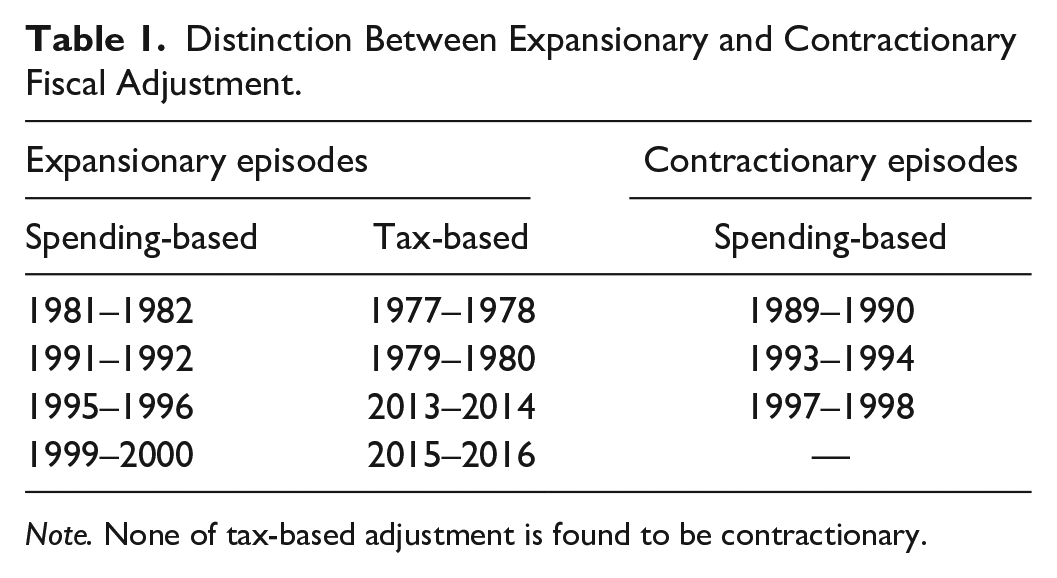
Note. None of tax-based adjustment is found to be contractionary.
The difference between GDP growth between expansionary and contractionary FA has been presented in Appendix A. From the results, it is evident that during expansionary FA, average GDP growth has increased to 5.641% from 4.321%, and at 1% level, this increase is found to be significant. During contractionary FA, average GDP growth has reduced from 6.109% to 3.079%, and the mean difference is significant.
Table 2 compares the selected macroeconomic variables during the expansionary and contractionary FA. From the results, it is clear that during the expansionary FA, the average GDP growth has increased to 5.641% from 4.321%, and this increase is found to be significant. During the contractionary FA, the average GDP growth has reduced from 6.109% to 3.079%, and the mean difference is significant. The average debt/GDP ratio during expansionary FA is significantly lower than that of the contractionary ones. Remarkably, the expansionary FA results in deteriorating the public finance and raises the debt/GDP ratio by 4.889 percentage points on average after 2 years of the adjustment. On the contrary, contractionary FA reduces the debt/GDP ratio by 1.142 percentage points; however, the difference between the expansionary and contractionary adjustments is statistically insignificant. The average GDP growth during the expansion is 6.738% as compared with contractionary FA with 3.080%, and the difference between the two growth rates is significant. Differences in averages of the current account balance, inflation, unemployment, short-term interest rate (call money rate), and the overall fiscal balance are statistically insignificant when comparing the expansionary FA with the contractionary ones. The average primary fiscal deficit during the expansion is higher than that of the contraction, and the difference is significant at 1% level. Similarly, the average real effective exchange rate (REER) during the expansionary FA is higher than that of the contractionary ones, and the difference is highly significant.
Macroeconomic Variables During Expansion and Contraction.

Note. GDP = gross domestic product; REER = real effective exchange rate.
and ** indicate significance at 1% and 5% levels of probability, respectively.
Dynamic Analysis of the Impact of the FA
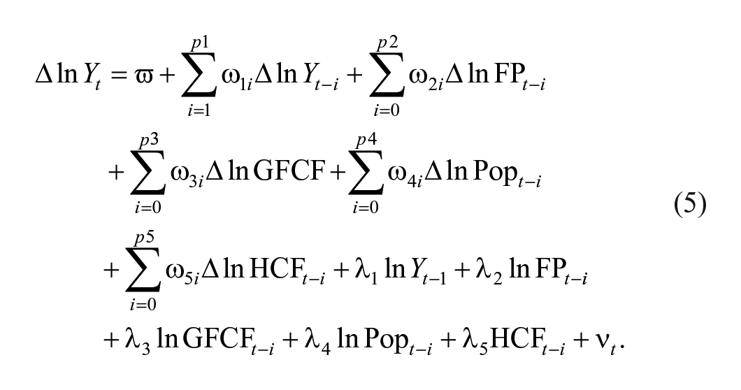
The dynamic analysis of the impact of the FA is done under the framework of Mankiw et al.’s (1992) model. The variable of FA is constructed while keeping in view the definition of Alesina and Ardagna (2013). First, the true fiscal stance is identified and a categorical variable is introduced, taking the value of “1” in each year if the CAPB improves in 2 consecutive years, and “0” if otherwise; this dummy variable is then multiplied by the series of CAPB. Some authors (Alesina & Ardagna, 2013; R. Banerjee & Zampolli, 2019) argue that cyclical adjustment with the primary fiscal balance via Hodrick–Prescott (HP) filter may fail to isolate the discretionary fiscal stance that would be completely exogenous to macroeconomic conditions. Therefore, a sizable reduction in the CAPB should be used to proxy the true fiscal stance. Besides this, the omitted variables such as asset prices (Guajardo et al., 2014) may influence the situation. However, some influential studies (Devries et al., 2011; Jordà & Taylor, 2016) insist to use the narrative approach toward the identification of FA. The narrative approach involves the identification of adjustment episodes based on policy shifts in fiscal variables identified in pre-budget speeches in the parliament by president/other government officials. Guajardo et al. (2014) have also suggested this approach. According to these studies, the narrative approach cures the problems of endogeneity and measurement errors. Besides this, the approach is expected to make estimates of OLS not only unbiased but also consistent. The development of such narrative approach toward the identification of FA—in the case of Pakistan for more than 40 years—would require sufficient funds and human resources, and hence is beyond the limit of this study. However, attempt has been made to cure the problems of endogeneity and measurement by applying the ARDL techniques. A weak exogeneity test has been conducted to test whether the policy instrument (in this case FA) is weakly exogenous or not. Besides this, the degenerate cases have been probed which may arise in the application of the ARDL techniques. Two separate models have been calibrated on Mankiw et al.’s (1992) model: the one investigating the effect of FA via a model denoted by SIZEFA, and the other estimating the composition of FA via the model represented by COMFA. Both the models are estimated through the Linear Autoregressive Distributed Lag (LARDL) techniques. Appendix B reports data sources, whereas the construct of the variables is shown in Appendix C.
There are certain tests that are frequently used by researchers in time-series analyses. Among these, we apply Phillips–Perron (PP) test besides the famous Dickey–Fuller Generalized Least Squares (DF-GLS), and the results are shown in Appendix D. As the observations suggest that often most of the macroeconomic aggregates remain I(0) or I(1), pre-testing is not a big deal within ARDL techniques (Bahmani-Oskooee et al., 2018). However, unit root tests have been conducted to confirm that none of the underlying variables is I(2). The ARDL techniques cannot be applied in such a situation (Pesaran et al., 2001). It has been shown that Augmented Dickey Fuller (ADF) test is not reliable in the small sample studies (DeJong et al., 1992; Elliot et al., 1996; Harris, 2009) as is the case with our study.
In the present study, therefore, we applied DF-GLS and PP tests to check the stationarity of the variables of our interest. These tests indicate that five variables of our interest become stationary at first difference under the assumption of both “drift” and “drift & trend.” Such variables include log of per capita income (denoted by LPCI), population growth (denoted by GPOP), gross fixed capital formation (denoted by GFCF), and CAPB and spending (denoted by CAPB and log of cyclically adjusted primary spending [LCAPS], respectively). Only two variables are found stationary at levels on the basis of the DF-GLS test when “drift & trend” was taken into account. These variables are secondary school enrollment (denoted by growth of secondary school enrollments [GSSE]) and CAR (denoted by log of cyclically adjusted revenue [LCAR]). GSSE remained consistent, but LCAR carried unit root at the level under the assumption of “drift.” On the contrary, the PP test indicates a somewhat different conclusion. Under the assumption of “drift” two variables (GFCF and GSSE) are found stationary at levels, while the rest carried unit root at levels. Only GSSE remained consistent over both the tests. In brief, we found that none of the underlying variables is integrated of Order 2; hence, the application of the ARDL techniques is justified in the present case. Under the SIZEFA model, the bound F value (14.420) lies well above the upper critical value at 1% level of probability. We have reported the F value in Table 3, which confirms the long-run relationship between the FA and growth.
Bound F Test of SIZEFA and COMFA Models.
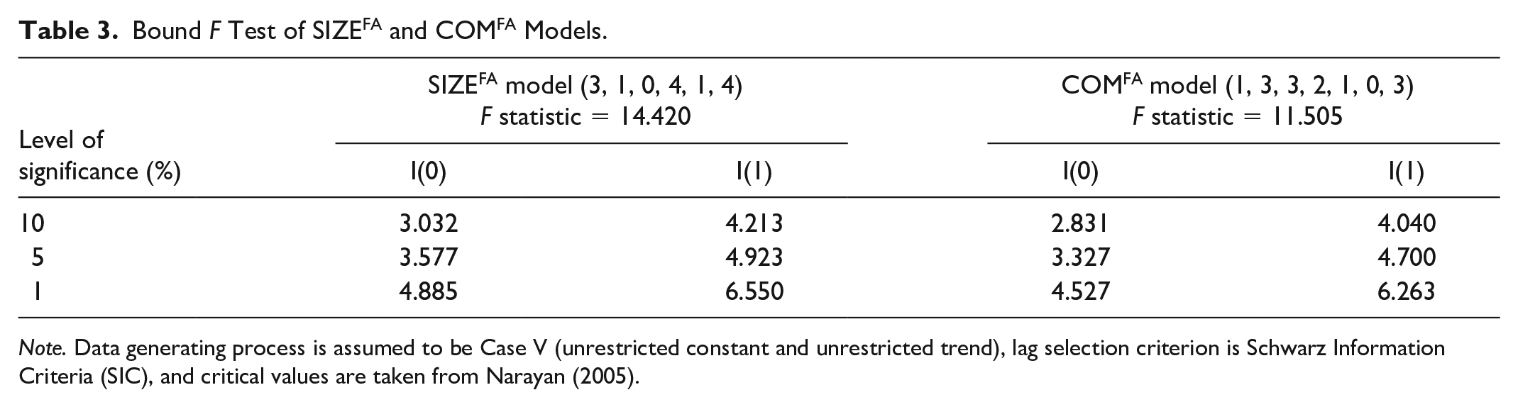
Note. Data generating process is assumed to be Case V (unrestricted constant and unrestricted trend), lag selection criterion is Schwarz Information Criteria (SIC), and critical values are taken from Narayan (2005).
To avoid the omitted variable bias, other important ingredients of growth like GFCF, secondary school enrollments, and population have been incorporated in the model. The F value (11.505) under COMFA model (shown in Table 3) is above the critical value at 1% level, thereby confirming the co-integrating relationship. The Degenerate Case I and Degenerate Case II have been tested, and the results are shown in Table 4. The calculated value of t statistic of SIZEFA model is −7.640, while it is −6.270 for the model of COMFA. Both are significant at 1% probability level. Test results of the Degenerate Case I for both the models are significant at 5% and 1% levels in case of SIZEFA and COMFA models, respectively. Unlike other studies, this study takes a special care of the degenerate cases arising in the application of ARDL.
Degenerate Case I and Degenerate Case II of SIZEFA and COMFA Models.
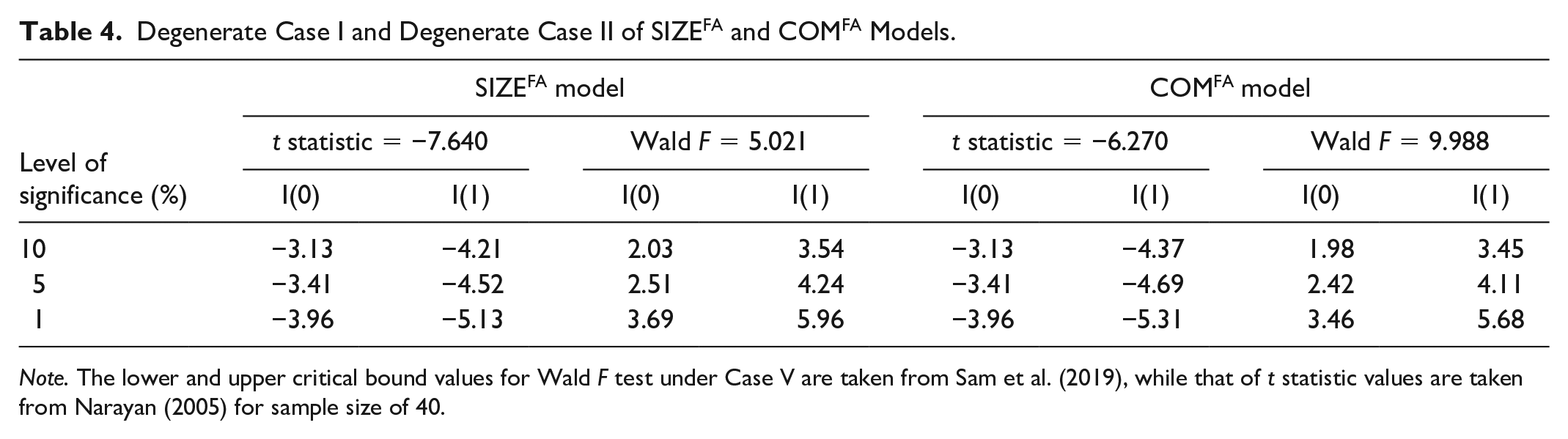
Note. The lower and upper critical bound values for Wald F test under Case V are taken from Sam et al. (2019), while that of t statistic values are taken from Narayan (2005) for sample size of 40.
Similarly, the weak exogeneity test is conducted via likelihood ratio (LR). This statistic follows chi-square distribution, and the results for both models are presented in Table 5. The results under SIZEFA model indicate that CAPB during periods of FA, denoted by CAPBFA, is weakly exogenous at 10% level of probability; while the CAPB (denoted by CAPB during periods of no adjustment) is weakly exogenous at 1% significance. In the model of the composition of FA (COMFA), CAPS during periods of no FA (denoted as CAPS) is weakly exogenous at 1%, while CAPS during periods of FA (denoted as CAPSFA) is insignificant at 10% level of probability. Likewise, CAR during FA (denoted as CARFA) is weakly exogenous at 10% probability, but the LR test shows that during periods of no adjustment, it is not weakly exogenous at even 1% level of probability.
Weak Exogeneity Test (Likelihood Ratio) for SIZEFA and COMFA Models.

The Granger causality/blocked exogeneity test under vector error correction model (VECM) of the ARDL techniques is reported in Appendix E. The test indicates that CAPB Granger-causes the economic growth at 5% level of probability and hence evidences strong exogeneity. Moreover, this causation is unidirectional and runs from CAPB to the economic growth. Surprisingly, CAPBFA does not Granger-cause the economic growth, and the tests show no causation in either way at the standard level of probability. This confirms that CAPBFA remains weakly exogenous. However, the test for the composition of FA points no causality running in either way, in case of both CAPSFA and CARFA, toward the economic growth at 10% level of significance. Both the public spending (CAPSFA) and the public revenue (CARFA) during the periods of FA are found to be weakly exogenous.
The estimated long-run effects of FA over economic growth for both the models are reported in Table 6. Both the models are in the form of Log-Lin (Gujarati, 2005, offers details on log-linear models), as only the dependent variables are in log form. Moreover, to analyze the influence of the size of FA on growth, a dummy variable was created taking the values of “1” if there is sizable reduction in CAPB (based on Definition 1) and “0” if otherwise, and then the dummy was multiplied by the series of CAPB. The coefficient associated with this new variable is the differential slope coefficient, showing the difference between the impact of the fiscal policy during the periods of FA and periods of nonadjustment.
Long-Run Estimates of SIZEFA and COMFA Models.

Note. CAPB = cyclically adjusted primary balance; CAPS = cyclically adjusted primary spending; CAR = cyclically adjusted revenue; GGFCF = growth of gross fixed capital formation; GSSE = growth of secondary school enrollments; POPG = population growth.
Following Yip and Tsang (2007), there are two equivalent approaches of entering the slope dummy in a regression equation: the base specification and the partition specification. Technical details on these approaches can be found in the study of Yip and Tsang (2007). As the regression takes the form of log-linear model, the impact of each explanatory variable should be interpreted after multiplying them by 100. Similar adjustment has been made with the model investigating the effect of composition of FA on growth. The coefficient associated with CAPB is the estimated impact of the base category during the periods of non-FA in this case—also termed as “the main effect.” Similarly, the associated coefficient with CAPBFA measures the differential effect between the two periods. The coefficient of CAPB, after multiplying by 100, is −2.50; while that of CAPBFA is 1.00. Both coefficients are highly significant. To calculate the effect of the FA on economic growth, the coefficients associated with CAPB and CAPBFA are summed, which is equal to −1.50.
It is important to mention that the positive coefficient associated with CAPBFA does not necessarily implies that fiscal consolidation is growth enhancing; rather it simply indicates that the impact of fiscal austerity is less contractionary during periods of FA as compared with periods of no adjustment. Alternatively, this may indicate that governments normally go for austerity measures when the economy suffers from low growth stemming from unsustainable public debt. This finding confirms the findings of the studies of Alesina and Ardagna (2010, 2013) and Leibrecht and Scharler (2013), which are of the view that initial conditions of the economy may influence the outcomes of austerity. The growth effect of the fiscal deficit is negative as shown by many studies in Pakistan, including Ali and Ahmad (2010), Kakar (2011), Fatima et al. (2011), and Nazir et al. (2013). Other recent attempts by Qasim et al. (2015) and Hussain et al. (2017, 2020) have also shown similar conclusions for Pakistan. In a nutshell, the fiscal consolidation is expected to have positive effect on the growth in Pakistan or, at least, is less contractionary. Remarkably, the findings of the current study support the hypothesis of the expansionary fiscal contraction in the long run.
Besides estimating the impact of FA on the economic growth, the current study also estimated the effect of the composition of the FA to test the claim of the previous studies—mostly gathered around the developed and emerging economies. To ascertain whether the spending-based consolidation is expansionary, or whether it is the tax-based adjustment that expedites the growth, we estimated two models by splitting the CAPBFA into CAPS (CAPSFA) and CAR (CARFA) during the periods of FA. Similarly, the variable capturing the main effect (CAPB) is replaced by CAPS and CAR. This model was also estimated with the ARDL techniques. In the model of composition of FA, the explanatory variable of population growth is dropped as it was creating problem of multicollinearity in the model. The bound F test, reported in Table 3, indicates the existence of co-integrating relationship. Again, the F value, which is 11.505, exceeds the upper critical bound value at 1% level of significance. Recalling that the model was in Log-Lin form and the entry of dummy variables in the equation takes the form of base specification. The coefficient associated with CAPSFA is 0.70 after multiplication by 100 and is found to be significant at 10%. The coefficient of CAPS which shows the impact of the public spending during the periods of no FA is −2.50 after multiplying it by 100. This coefficient is found to be highly significant. Again, the sum of these two coefficients indirectly gives us the impact of the public spending in the periods of FA which is equal to −1.80. This shows that public spending on average is less contractionary during the periods of FA than during non-FA. In other words, one can declare that the spending-based consolidation is growth enhancing. The estimated coefficient of CARFA is −0.50 after multiplying it by 100, which is statistically insignificant. However, the coefficient of CAR is 5.2 after multiplying it by 100 and is highly significant. The sum of these two coefficients is equal to 4.7 and hence reveals that the fiscal consolidation through the tax hike is slightly growth retarding.
The speeds of adjustment toward equilibrium as measured by ECM terms are found significant in the case of both models. Table 7 reports these results. The ECM term of SIZEFA model is −0.841 which shows that 84.1% adjustment toward the equilibrium is restored each year after a shock occurs, while it is −0.639 for the model of composition of FA (COMFA) which indicates that 63.9% error is corrected each year. The bound critical values of ECM terms for both models have been reported in Table 8. The short-run impact of FA in the SIZEFA model is not visible, while in COMFA model it is more meaningful. The short-run coefficient attached with CAPSFA is statistically insignificant in the first period when FA was initiated, thereby implying that the spending-based adjustment does not improve growth. In the next two periods, the spending-based consolidation actually reduces the growth and such reductions in the two periods are significant at 1% probability. However, revenue-based consolidation is found to improve growth in the first period, but it is statistically insignificant.
ECM Estimates of SIZEFA and COMFA Models.

Note. The bound critical values for ECM terms are reported in Table 8. ECM = error correction model; CAPS = cyclically adjusted primary spending; CAPB = cyclically adjusted primary balance; CAR = cyclically adjusted revenue; GSSE = growth of secondary school enrollments; POPG = population growth; LRPCI = log of real per capita income.
The p value is not compatible.
ECM t-Bound Test of SIZEFA and COMFA Models.

Note. ECM = error correction model; CAPB = cyclically adjusted primary balance.
Like the study of De Cos and Moral-Benito (2013), our study arrives at the conclusion that when FA is considered as weakly exogenous, then one could find FA to be contractionary in the short run. Other recent studies by Jordà and Taylor (2016) and R. Banerjee and Zampolli (2019), employing the local projection methods, show similar conclusions and find fiscal austerity to be recessionary in the short run in the case of OECD countries. Jordà and Taylor (2016) further demonstrate that 1% fiscal austerity leads to a fall in the GDP growth by 3.50% in the next 5 years. Unlike OLS method, ARDL techniques applied in the current study allow feedback effect of the dependent variable. Such effect is captured by incorporating sufficient lags of the dependent variable as regressors while estimating the short- and long-run effects. This study confirms such contractionary effect of the size of FA in the short run only while evidences expansionary effect in the long run.
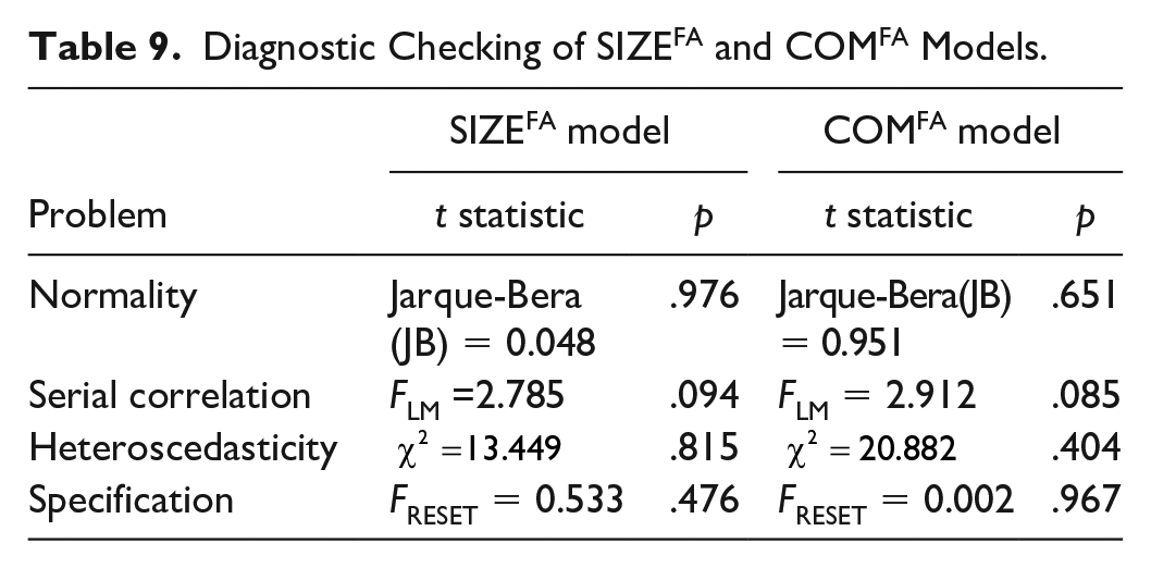
The long-run effect of the size of FA is inconformity with the established notion surrounding the hypothesis of “expansionary fiscal contraction.” This econometric evidence is remarkably inconformity with the findings of Alesina et al. (2002) and Alesina and Ardagna (2010, 2013). The common point of these studies is that all ascertain the expansionary fiscal contraction in the short run only but did not probe it in the long run. This may be counted as another advantage of the current study. Table 9 reveals diagnostic checking of both the models. The results show that none of the conventional problems is found in the models. The assumption of normality was tested via Jarque–Bera statistic, whereas LM test was conducted to check autocorrelation. Furthermore, the problem of heteroscedasticity is not present in both models, and the test is conducted through Breusch–Pagan–Godfrey (BPG) test. The test does not reject the assumption of homoscedasticity at 10% significance level for both models. The Ramsey Regression Equation Specification Error Test (RESET) indicates that both models are correctly specified at 10% significance level. Stability test of SIZEFA and COMFA models via square of Cumulative Sum (CUSUM) shows that the parameters are stable, and the results are reported in Appendices F and G, respectively. For testing the parameter stability, the study reports only tests of CUSUM square. As the slopes dummies have been used in both the models, the power of the square of CUSUM would be high and reliable as compared with a simple test of CUSUM, as advocated by Turner (2010).
Diagnostic Checking of SIZEFA and COMFA Models.
Conclusion and Policy Recommendation
This study endeavors to investigate the hypothesis of “expansionary fiscal contraction” in the context of Pakistan. Although it is intrinsically hard to isolate the macroeconomic impact of fiscal policy as other associated policies are often involved, attempt has been made to disentangle the impact of discretionary fiscal stance on economic growth to distill practical policy lesson. Using Definition 2 regarding fiscal austerity to be expansionary or contractionary, it is worth noting that eight periods are expansionary and three are contractionary. Evaluating the composition of the FA, seven periods of FA were spending-based and only four were tax-based. Further inquiry shows that the expansionary FA were half spending- and half tax-based; however, tax-based adjustments were not found to be contractionary.
Besides the descriptive analyses of the FA, the study attempted to empirically estimate the effect of both the size and composition of the FA in enhancing the growth in the country. Following the definition of the FA of Alesina and Ardagna (2013), the empirical model has been calibrated on Mankiw et al.’s (1992) model and estimated via the ARDL techniques. Following Yip and Tsang (2007), the current study adopted the base specification of slope dummy in the models. The merit of the present study over these studies, however, lies in the attempt to investigate the impact of the composition of FA on growth in both the long and short runs. This implies that the spending-based adjustment enhances the economic growth, while the tax-based adjustment is likely to be growth retarding in the long run. In line with De Cos and Moral-Benito (2013), this study arrives at the conclusion that when the FA is considered as weakly exogenous, then one could find the FA to be contractionary in the short run.
It is worthy to note that the positive coefficient associated with the CAPB (the size effect) during the periods of the FA does not necessarily imply that the fiscal consolidation is growth enhancing. Rather it simply indicates that the impact of the fiscal austerity is less contractionary during the periods of the FA as compared with the periods of no adjustment. Equivalently, one may declare such austerity measures to be growth enhancing.
The outcomes of this study show interesting insights into the issue of the fiscal deficit at both the aggregated and disaggregated levels, and their macroeconomic consequences on the economic growth. As our analysis shows that the size of the fiscal deficit is growth retarding in the country, urgent austerity measures would be required. Such measures should aim to reduce the size of the fiscal deficit to a manageable level to overcome its growth consequences. Two approaches have been identified in the discipline of public finance to curtail the overall size of the deficit. In such like situations, many countries have applied the strategy to decrease spending and/or increase taxes to minimize the adverse effects. However, each approach has its own pros and cons. For example, growth will be compromised when public spending is excessively curtailed or the tax rate revised. The fiscal authority is left with the strategy of smart consolidation measures, which could switch the fiscal restraints into the opportunity of growth and development. To put public finance on a sustainable path and to overcome the adverse macroeconomic impacts of the unsustainable public debt arising from large fiscal deficits, the fiscal managers should go for spending-based austerity measures. Moreover, twisting the composition of the public spending in favor of the capital spending is expected to enhance economic growth and will help achieve the Millennium Development Goals in the country.
Footnotes
Appendix A
Difference Between Average GDP Growths (Definition 2).

| Expansionary | Contractionary | ||||||
|---|---|---|---|---|---|---|---|
| Episodes | Before (1) | During (2) | Change (2) – (1) | Episodes | Before (1) | During (2) | Change (2) – (1) |
| 1977–1978 | 4.684 | 5.998 | 1.314 | 1989–1990 | 7.039 | 4.709 | −2.330 |
| 1979–1980 | 5.998 | 6.987 | 0.989 | 1993–1994 | 6.384 | 2.747 | −3.636 |
| 1981–1982 | 6.987 | 7.229 | 0.242 | 1997–1998 | 4.904 | 1.782 | −3.122 |
| 1991–1992 | 4.709 | 6.384 | 1.674 | — | — | — | — |
| 1995–1996 | 2.747 | 4.904 | 2.157 | — | — | — | — |
| 1999–2000 | 1.782 | 3.960 | 2.178 | — | — | — | — |
| 2013–2014 | 3.128 | 4.535 | 1.407 | — | — | — | — |
| 2015–2016 | 4.535 | 5.129 | 0.594 | — | — | — | — |
| Average | 4.321 (0.606) | 5.641 (0.420) | 1.320 (0.245)* | Average | 6.109 (0.631) | 3.079 (0.861) | −3.030 (0.380)** |
Note. Standard errors are in parentheses. GDP = gross domestic product.
and ** indicate significance at 1% and 5% levels of probability, respectively.
Appendix B
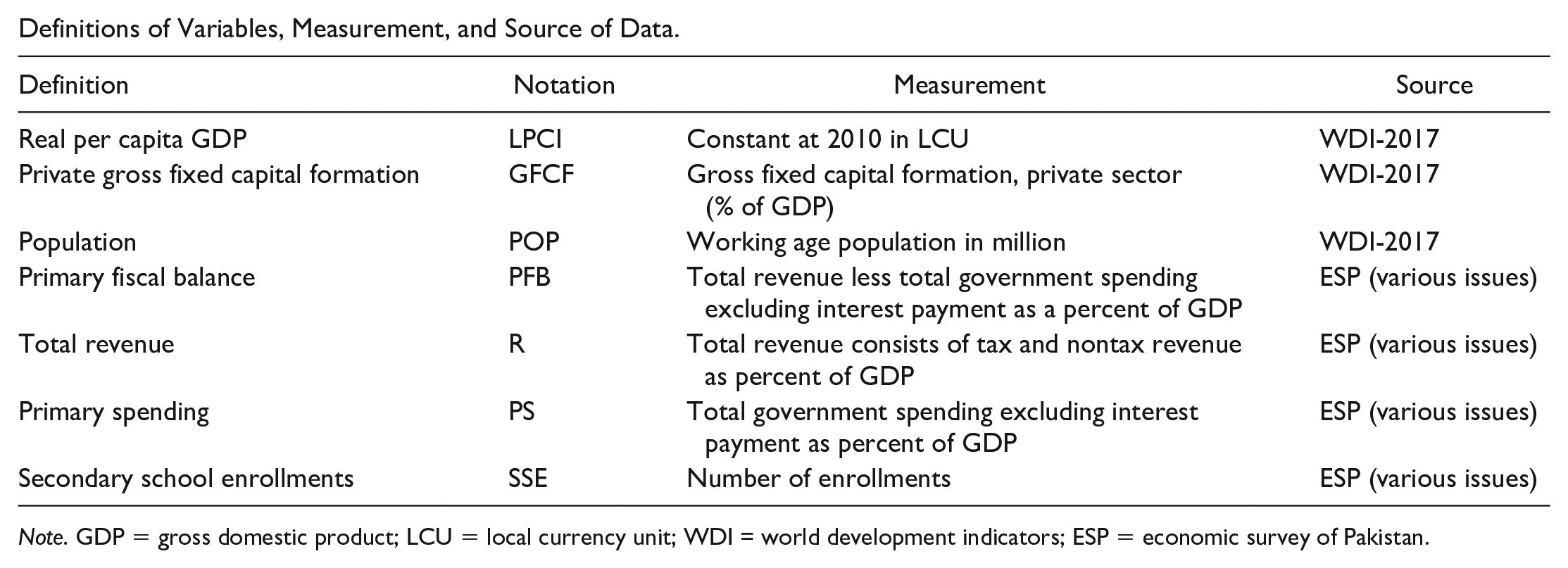
Definitions of Variables, Measurement, and Source of Data.
| Definition | Notation | Measurement | Source |
|---|---|---|---|
| Real per capita GDP | LPCI | Constant at 2010 in LCU | WDI-2017 |
| Private gross fixed capital formation | GFCF | Gross fixed capital formation, private sector (% of GDP) | WDI-2017 |
| Population | POP | Working age population in million | WDI-2017 |
| Primary fiscal balance | PFB | Total revenue less total government spending excluding interest payment as a percent of GDP | ESP (various issues) |
| Total revenue | R | Total revenue consists of tax and nontax revenue as percent of GDP | ESP (various issues) |
| Primary spending | PS | Total government spending excluding interest payment as percent of GDP | ESP (various issues) |
| Secondary school enrollments | SSE | Number of enrollments | ESP (various issues) |
Note. GDP = gross domestic product; LCU = local currency unit; WDI = world development indicators; ESP = economic survey of Pakistan.
Appendix C
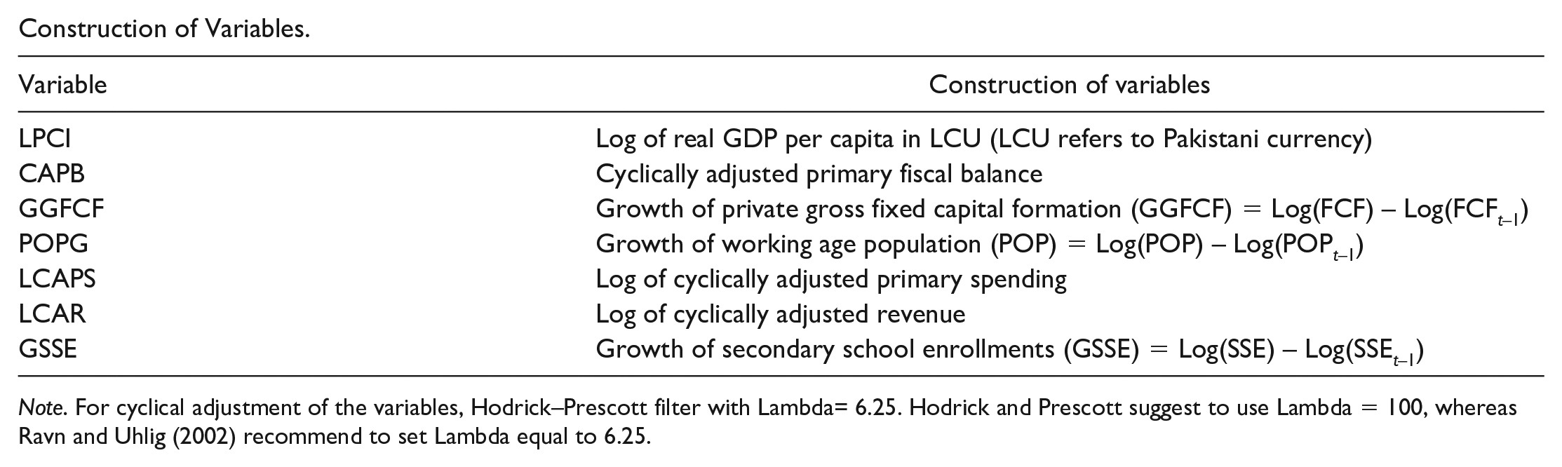
Construction of Variables.
| Variable | Construction of variables |
|---|---|
| LPCI | Log of real GDP per capita in LCU (LCU refers to Pakistani currency) |
| CAPB | Cyclically adjusted primary fiscal balance |
| GGFCF | Growth of private gross fixed capital formation (GGFCF) = Log(FCF) – Log(FCFt–1) |
| POPG | Growth of working age population (POP) = Log(POP) – Log(POPt–1) |
| LCAPS | Log of cyclically adjusted primary spending |
| LCAR | Log of cyclically adjusted revenue |
| GSSE | Growth of secondary school enrollments (GSSE) = Log(SSE) – Log(SSEt–1) |
Note. For cyclical adjustment of the variables, Hodrick–Prescott filter with Lambda= 6.25. Hodrick and Prescott suggest to use Lambda = 100, whereas Ravn and Uhlig (2002) recommend to set Lambda equal to 6.25.
Appendix D
Evidence From DF-GLS/Elliott, Rothenberg, and Stock (ERS) and PP Tests.

| Variables | DF-GLS | PP | ||||||
|---|---|---|---|---|---|---|---|---|
| Drift | Drift & trend | Drift | Drift & trend | |||||
| Level | Δ | Level | Δ | Level | Δ | Level | Δ | |
| LPCI | 0.59 | −4.46* | −2.12 | −4.60* | −1.23 | −4.67* | −2.35 | −4.80* |
| CAPB | −0.40 | −2.52** | −1.66 | −3.66** | −2.60 | −3.03** | −2.19 | −4.31* |
| GFCF | −1.07 | −2.13** | −2.13 | −6.38* | −2.69*** | −7.73* | −2.56 | −7.79* |
| GPOP | −0.20 | −4.87* | −1.73 | −5.64* | −0.22 | −5.60* | −1.84 | −5.65* |
| LCAPS | −1.12 | −7.09* | −1.71 | −7.29* | −1.65 | −7.25* | −1.51 | −7.28* |
| LCAR | −1.77** | −7.59* | −2.18 | −7.56* | −1.80 | −7.52* | −2.51 | −7.44* |
| GSSE | −7.03* | −7.78* | −7.32* | −7.84* | −7.06* | −20.56* | −7.16* | −20.25* |
Note. DF-GLS = Dickey–Fuller Generalized Least Squares; PP = Phillips–Perron; CAPB = cyclically adjusted primary balance; GFCF = gross fixed capital formation; POPG = population growth; LCAPS = log of cyclically adjusted primary spending; LCAR = log of cyclically adjusted revenue; GSSE = growth of secondary school enrollments.
, **, and *** indicate significance at 1%, 5%, and 10% levels of probability, respectively.
Appendix E
Vector Error Correction (VEC) Granger Causality Wald Tests (Summary).

| Variable | Granger-cause | Variable | Chi-square | Conclusion |
|---|---|---|---|---|
| ΔCAPB | → | ΔLRPCI | 7.623** (.022) | Unidirectional |
| ΔCAPBFA | → | ΔLRPCI | 1.830 (.401) | No causality |
| ΔCAPS | → | ΔLRPCI | 4.897*** (.086) | Unidirectional |
| ΔCAPSFA | → | ΔLRPCI | 0.644 (.725) | No causality |
| ΔCAR | → | ΔLRPCI | 17.430** (.000) | Unidirectional |
| ΔCARFA | → | ΔLRPCI | 0.261 (.878) | No causality |
| ΔGGFCF a | → | ΔLRPCI | 2.197 (.333) | No causality |
| ΔGSSE | → | ΔLRPCI | 6.055** (.048) | Unidirectional |
| ΔGPOP | → | ΔLRPCI | 4.624*** (.099) | Unidirectional |
Note. The p values are in parentheses. CAPB = cyclically adjusted primary balance; CAPS = cyclically adjusted primary spending; CAR = cyclically adjusted revenue; GGFCF = growth of gross fixed capital formation; GSSE = growth of secondary school enrollments; GPOP = population growth; LRPCI = log of real per capita income.
Indicates that causality runs from LRPCI to GGFCF with chi-square statistic =19.744 which is significant at 1% level of significance.
and *** indicate significance at 5% and 10% levels of probability, respectively.
Appendix F
Appendix G
Declaration of Conflicting Interests
The author(s) declared no potential conflicts of interest with respect to the research, authorship, and/or publication of this article.
Funding
The author(s) received no financial support for the research, authorship, and/or publication of this article.