Sage Journals: Discover world-class research

Abstract

The current study attempts to explore the determinants of CO₂ emissions per capita considering spatial effects for a panel of 21 North American countries. The results corroborate the existence of spatial dependence in per capita carbon dioxide emissions and its determinants. Adverse environmental spillover effects are found for all hypothesized determinants while per capita income showed a positive impact. Furthermore, the existence of environmental Kuznets curve hypothesis is proven with a turning point of 15,665 constant U.S. dollar per capita income, and 6 of the 21 investigated countries are found at the second stage of an inverted U-shaped relationship. An inverted U-shaped relationship between trade openness and carbon dioxide emissions per capita has also been found. Financial market development (foreign direct investment) seems to have monotonic positive (negative) effects.

Keywords

environmental Kuznets curve hypothesis income per capita financial market development foreign direct investment trade openness spatial dependency North America

Introduction

With the growing risks of global warming, the ecological systems across the world are exposed to a wide range of issues if sufficient measures are not adopted to maintain sustainable development (Ulucak et al., 2019). Among others, CO₂ emissions are considered to be among the most significantly crucial greenhouse gases that play a role in exacerbating global warming. Considering its long-lasting effects and 75% contribution to greenhouse gas volume, many international bodies are making efforts to reduce CO₂ emissions on a large scale. As an effort to that agenda, a global agreement of the United Nations Framework Convention on Climate Change (UNFCCC) has been initiated to reduce the greenhouse gases. The idea was further reinforced by two agreements: Kyoto Protocol and Paris Agreement as a sign of commitment to decrease greenhouse gases. Tai et al. (2015) mentioned air pollution to be one of the leading risk factors leading to deaths worldwide. In addition, economic activities and CO₂ emissions seem to go hand in hand because an economy with larger production volume will have possibly more substantial emissions, leaving space for rigorous environmental policy formation (Ajmi et al., 2015). Despite the shift to renewables, coal retirements, and replacement of clean power plan with affordable clean energy in some of the North American countries, there is still much space to look for improvements in its environmental policy structure to promote a cleaner environment.

The United States, Canada, and Mexico signed a North American Free Trade Agreement (NAFTA) to promote trade and to curb its environmental effects, and a supplement North American Agreement on Environmental Cooperation (NAAEC) was also signed. Grossman and Krueger (1991) conducted a pioneer research to find the environmental effect of NAFTA and argued that Mexico gained economic growth from NAFTA. From a cross-country analysis, they found the negative environmental effects of economic growth in low-income countries and the positive environmental effect for high-income ones. A turning point from negative to positive environmental effect starting from US$4,000 to US$5,000 per capita income was suggested. Following this idea, some seminal studies corroborated the environmental Kuznets curve (EKC) hypothesis in groups of developed and developing countries (Grossman & Krueger, 1995; Selden & Song, 1994; Shafik & Bandyopadhyay, 1992).

NAFTA aims to promote the trade and the investment among the member countries. Canada and Mexico are the largest energy trading partners of the United States and also the major trading partners of other products. Mexico is the largest producer of petroleum and other liquids in the world and Canada is also among the top five energy producers in the world (Energy Information Administration, 2019). In the environmental profile, the United States is the second largest emitter of total CO₂ emissions in the world after China. Mexico and Canada also fall in the top 12 emitters of CO₂ emissions (Union of Concerned Scientists, 2019). The NAFTA trading bloc may have environmental consequences of foreign investment and trade as NAFTA is an agreement between the developed and developing countries, and dirty industry or production process may shift from developed to developing country to take advantage of lax environmental regulation (Copeland & Taylor, 1995). This phenomenon gives birth to the pollution haven hypothesis (PHH).

The environmental consequences of NAFTA are not just limited to the members’ countries but may have environmental consequences for other nearby located developing countries in the North America. Moreover, the spatial effects of pollution emissions cannot be ignored due to the geographically closely located countries in the North American region. Maddison (2006) argues that neighboring developing countries are facing the competition in attracting the investment and the trade from the developed countries which is also responsible for spatial dependency of pollution emissions. Dinda (2004) claims that variations in the results of pollution emissions’ models are due to different specifications while choosing the relevant variables. The estimated nonspatial model in the presence of statistically significant spatial effects can be claimed for specification biasness (Anselin, 1988). Therefore, the spatial dependency should not be ignored in the pollution model of the North American region with nearby located countries.

The North American region is consisted of a mix of developed and developing countries, and trade openness, foreign direct investment (FDI), and financial market development (FMD) could form the PHH in the region. Hence, it is very important to see the net environmental impact of these variables on the pollution emissions of the whole region. Anastacio (2017) investigated the EKC in three NAFTA countries, and other studies investigated the EKC hypothesis in the single-country case of the NAFTA region (e.g., Burnett, Bergstrom, & Wetzstein, 2013; Dogan & Turkekul, 2016; Lantz & Feng, 2006; Lipford & Yandle, 2011; Olale et al., 2018). Other than EKC, some studies also investigated the role of FDI, trade, and FMD in the pollution emissions in the single-country analysis of the NAFTA region (Dogan & Turkekul, 2016; Gale, 1995; Shahbaz et al., 2019; Waldkirch & Gopinath, 2008). But, the role of the mentioned variables in the pollution emissions of the whole North American region is missing in the literature, and spatial dependency of pollution emissions of this region also needs attention. To bridge this literature gap, this present study is targeted to find out the effects of per capita income, FDI, FMD, and trade openness on the per capita CO₂ emissions of the North American region. To ensure the significant contribution to the literature, spatial dependency and expected quadratic relationships are also cared in the CO₂ emissions’ model.

Literature Review

There is a vast literature available on the EKC hypothesis testing. For example, Acaravci and Akalin (2017) probed the EKC in the panel of developed and developing countries for the period 1980 to 2010. They validated the EKC in the developed countries but could not find this evidence for developing countries. Furthermore, trade openness of developing countries showed a negative effect on CO₂ emissions, but the impact of trade openness was found insignificant in the panel of developed countries. Using a period 1980 to 2012, Shahbaz et al. (2015) examined the EKC for some countries of Sub-Saharan Africa and validated the EKC in the panel and some of the individual countries’ analyses as well. Moreover, they reported the positive effect of energy intensity on the CO₂ emissions and bidirectional causality between CO₂ emissions and economic growth. Using a period 1990 to 2011, Apergis and Ozturk (2015) validated the EKC in a panel of 14 selected Asian countries. They also found the inverted U-shaped relationship in industrial share and CO₂ emissions, and most of the investigated institutional quality indicators showed a negative effect on the CO₂ emissions.

In their analysis, Ozturk and Acaravci (2013) corroborated the EKC hypothesis for the Turkish economy using data from 1960 to 2007. Furthermore, they reported that trade openness accelerated CO₂ emissions, but financial development showed an insignificant effect. Using the period 1971 to 2014, Pata (2018) revisited the EKC in Turkey and confirmed the validity of EKC. However, he found Turkey on the first stage before the turning point of EKC. Moreover, he reported positive effects of financial development, industrial output, imports, urban population, and coal use, and negative impacts of noncarbon energy use and exports on the CO₂ emissions. Mahmood et al. (2018) investigated and validated the EKC in Saudi Arabia using the period of 1971 to 2014. They found Saudi Arabia in the first phase of EKC and reported a negative relationship between decreasing financial development and CO₂ emissions in the asymmetry analysis.

Later, we focus on the Americas region, and the studies on Latin American and Caribbean countries are discussed at first. For example, Bhattarai and Hammig (2001) examined the EKC hypothesis and the determinants of deforestation for a panel of 20 Latin American countries along with Africa and Asia regions. They found an N-shaped relationship between income and deforestation in Latin America. Political institution, change in cereal yield, and population growth showed negative impacts on deforestation, but black market, rural population density, and debt illustrated positive effects. Martinez-Zarzoso and Bengochea-Morancho (2003) utilized dynamic econometric techniques on the isolated relationship between CO₂ emissions per capita and income per capita for a panel of 19 Latin American countries and found the U-shaped relationship. Poudel et al. (2009) investigated the EKC hypothesis using parametric and semiparametric estimation techniques for a panel of 15 Latin American countries. Parametric model suggested an N-curve relationship between CO₂ emissions and income. In addition, forestry seemed to play a role in reducing CO₂ emissions.

Sapkota and Bastola (2017) explored the determinants of CO₂ emissions for 14 Latin American countries and confirmed the validity of the EKC hypothesis. They also found positive effects of FDI, energy use, capital, and population dependency and negative effect of unemployment on CO₂ emissions. Also, they split their analysis for the sample countries’ income per capita less than and more than US$3,550. In the split results, positive effect of FDI was found to be more significant for “income less than US$3,550.” In low-income countries, the relationship was U-shaped instead of inverted U-shaped while being insignificant for high-income countries. This finding is matched with the arguments of Birdsall and Wheeler (1993) who rejected the PHH and claimed that trade liberalization and foreign investments have encouraged clean industries in the Latin America through cleaner standard of developed countries. In the same line, while investigating U.S. outbound FDI, Eskeland and Harrison (2003) mentioned that in comparison with local competitors, foreign investors seem to put lesser pressure on the environment due to their energy-efficient technologies. However, Blanco et al. (2013) investigated the causality between sector-specific FDI and CO₂ emissions per capita for 18 Latin American countries and concluded that FDI in already polluted industries significantly caused the CO₂ emissions.

Anastacio (2017) investigated EKC for three NAFTA partners and validated the existence of the EKC hypothesis and positive environmental effects of electricity consumption. Using historical data of a period 1800 to 2011, Henriques and Borowiecki (2017) examined the income–CO₂ relationship for America and Canada along with some European countries and Japan. They found that a low level of income and switching from biomass to fossil energy consumption contributes to CO₂ emissions, while technology helps in reducing CO₂ emissions. Guevara et al. (2019) claimed that energy and nonenergy trade of the NAFTA countries transformed this bloc into an integrated energy system. The United States provided the Mexican energy demand with lesser efficiency. Therefore, Mexico could not perform efficiently in the energy sector as compare with her partners’ countries. However, efficient energy supply chain was observed between the United States and Canada due to more integration and the same level of development. Overall integrated energy trade helped to reduce CO₂ emissions in the region. Furthermore, they found that CO₂ emissions are transferred from Canada and Mexico to the United States which also provides an evidence for spatial dependence of emissions in the region.

Ameyaw et al. (2019) studied the economic growth of selected countries, including the United States and Canada, and analyzed the link between CO₂ emissions from fossil fuel combustion. A long-term relationship was established between gross domestic product (GDP) growth, trade, and CO₂ emissions. They found the unidirectional causality from economic growth to CO₂ emissions from fossil fuel in Canada and the United States. Essandoh et al. (2020) investigated 52 countries including the United States, Canada, and Mexico and linked international trade and FDI with CO₂ emissions. They found that trade helped to reduce CO₂ emissions in developed countries and FDI has positive impact on CO₂ emissions in the developing countries.

Soytas et al. (2007) mentioned that while income does not have any causal impact on emissions in the United States, energy consumption increases it. Burnett, Bergstrom, and Wetzstein (2013) questioned the idea of incorporating energy variables in the study and compared the EKC model for the United States with and without energy variable from 1981 to 2003. Using heating degree days (HDDs) and cooling degree days (CDDs) as control variables, they found an evidence of EKC in the model with energy variable. However, the effect of income and its square has been reported insignificant without energy variable. Introducing structural breaks in the quarterly time series of the United States, Congregado et al. (2016) reinvestigated the income–CO₂ emission relationship and found EKC existent in all sectors except industrial. Cherniwchan (2017) tested the effects of trade liberalization due to NAFTA on U.S. manufacturing and showed that emissions have significantly reduced from U.S.-based power plants.

Dogan and Turkekul (2016) found a U-shaped relationship between income and emissions in the United States from 1960 to 2010. Energy consumption and urbanization showed a positive impact, whereas trade openness illustrated negative impacts on pollution, and effect of FMD was insignificant. Using a period 1966 to 2013, Aslan et al. (2018) reinvestigated the EKC in the United States using a bootstrap rolling window and found the evidence of EKC in the United States with increasing and decreasing trends of the coefficient of economic growth in the two subperiods 1982 to 1996 and 1996 to 2013, respectively. Alola (2019) explored the influence of policies on the pollution emissions of the United States from 1990 to 2018. He found that monetary and trade policies and financial regulations contributed to the CO₂ emissions. Shahbaz et al. (2019) mentioned that energy consumption, trade openness, and FDI have an influence on CO₂ emissions in the United States. Energy consumption and FDI increase CO₂ emissions, whereas trade openness declines CO₂ emissions.

Using state-level data, Carson et al. (1997) investigated seven types of air pollution–per capita income relationship in 50 U.S. states and found a negative association. Aldy (2005) corroborated the EKC hypothesis using U.S. state-level data from 1960 to 1999 and augmented the model with HDD, CDD, and coal production variables. In the isolated relationship of emissions per capita and income per capita, Apergis et al. (2017) estimated the time series models for 48 U.S. states and validated the EKC hypothesis using a period 1960 to 2010 in 10 states. Using the same period 1960 to 2010, Atasoy (2017) reinvestigated the EKC hypothesis for 50 U.S. states using Augmented Mean Group (AMG) and Common Correlated Effects Mean Group (CCEMG) estimators and population and energy consumption as control variables. They confirmed the evidence of the EKC hypothesis for 30 states using AMG estimators with turning points between US$1,292 and US$48,597 and 10 states using CCEMG estimators with turning points between US$2,457 and US$14,603.

Assuming nonlinear effects of income, population, and technology, Lantz and Feng (2006) investigated the EKC hypothesis for a panel of five regions of Canada and found an inverted U-shaped relationship of fossil fuel CO₂ emissions with population. Olale et al. (2018) examined the EKC hypothesis for greenhouse gas emissions using provincial and territorial data of Canada from 1990 to 2014 and confirmed the existence of EKC but found an insignificant effect of trade openness on emissions. Kerr and Mellon (2012) investigated the determinants of CO₂ emissions of Canada with other Organisation for Economic Co-operation and Development (OECD) countries and reported that CO₂ emissions are affected by income, population, energy demand, and fossil fuel dependence. Pazienza (2019) claimed that FDI seems to have a declining impact on CO₂ emissions in developed countries and FDI is increased in the OECD region. Furthermore, he found that fuel-burning CO₂ decreased because FDI invited technological advancement in the host nation.

Gale (1995) tested the effect of trade liberalization due to NAFTA on the CO₂ emissions of Mexico and reported that CO₂ emissions increase as a result of elimination of tariffs because structure of production and consumption has been shifted toward emission-intensive products. In the same line, Waldkirch and Gopinath (2008) probed the impact of FDI on industrial pollution of Mexico due to lax environmental policies and supported the PHH. However, Lankao (2004) argued that Mexico is depending on primary exports unlike America and Canada and still has a comparatively lesser share of carbon emissions compared with other NAFTA countries. In the isolated relationship of income and pollution emissions, Lipford and Yandle (2011) investigated the EKC hypothesis, before and after NAFTA agreement, for different kinds of emissions of Mexico from 1980 to 2000 and found a positive relationship between pollution emissions and income per capita.

Bockstael (1996) discussed a need of inclusion of spatial dependency in the ecological economics. Following this idea, Maddison (2006) investigated the EKC hypothesis by augmenting spatial weight matrix in the estimated models of different pollution emissions per capita for 135 countries using data of years 1990 and 1995. Evidence of U-shaped relationships was found in most of the pollution emissions and significant spillover effects were also found. Wang et al. (2013) investigated the spatial effects of income and biocapacity on the ecological footprints of 150 countries. They did not validate the evidence of the EKC hypothesis and reported a positive linear effect of income and biocapacity on the ecological footprints but negative spillover effects of the same variables were found.

In case of the United States, Rupasingha et al. (2004) investigated the EKC hypothesis for U.S. counties using toxic release data and confirmed an existence of the EKC hypothesis in all models due to spatial dependency. Auffhammer and Steinhauser (2007) investigated the predictive ability of CO₂ emissions’ model using a period 1960 to 2001 for 50 U.S. states and reported that the predictive ability of the estimated model has been enhanced because of state-level data and spatial effects. Burnett, Bergstrom, and Dorfman (2013) examined the impact of income, energy prices, CDDs, and HDDs on per capita energy emissions of 48 U.S. states using a period 1970 to 2009. They validated the EKC hypothesis in the point, direct, and indirect estimates and reported negative effects of electricity and oil prices and positive effects of HDDs on the energy emissions per capita.

Many environmental scientists, that is, Pataki et al. (2006), Gregg et al. (2009), and Balshi et al. (2009), explained the existence of spatial dependency of emission-related pollution in the North America. Moreover, literature also signified the importance of spatial analysis in the pollution-related studies but the application of spatial dependency is still scant and somewhat ignored in the energy pollution literature (Burnett, Bergstrom, & Dorfman, 2013). Nevertheless, a vast abyss remains when it comes to the applicability of EKC in the whole North American context in the environmental and spatial literature and a need to fully understand how spatial dynamics play a role in EKC’s implications in the North American region. Hence, this present research contributes to the pollution literature by applying spatial econometrics in testing the EKC hypothesis for a panel of 21 North American countries using a period of 1990 to 2014.

Theoretical Background

To model, the determinants of CO₂ emissions, income, or economic growth are considered to be most influential because while targeting economic growth, nations may sacrifice the environment, leading to environmental degradation in the initial stage of growth. When a milestone of economic growth has been achieved, clean environment becomes a demand for the sake of a healthy nation, and clean technology can be utilized to meet the new need (Dinda, 2004). At first, Grossman and Krueger (1991) reported a nonlinear relationship between income per capita and sulfur dioxide emissions and suggested a turning point between negative and later positive environmental effects of income growth due to scale effect, technique effect, and composition effect.

Later, this nonlinear relationship was called the EKC hypothesis by Panayotou (1993) based on Kuznets’ (1955) advocated inverted U-shaped relationship. In the initial stage of development and first phase of the inverted U-shaped relationship, income growth is possible due to a higher consumption of inputs leading to more pollution termed as scale effect. One instance of this is a conversion of an agrarian economy into an industrial one when, after some time of growth, the industrial economies may convert to service sector for a desire of a sustainable environment which is termed as composition effect (Arrow et al., 1995). Moreover, increasing income may enable a country to invest in R&D to produce clean technology, termed as technique effect (Komen et al., 1997). The scale effect is dominant at first stage of EKC, and technique and/or composition effects become dominant later to form the inverted U-shaped EKC (Grossman & Krueger, 1991, 1995; Vukina et al., 1999). Thereafter, a number of studies have tested the EKC hypothesis to find the turning point (Aldy, 2005; Atasoy, 2017). Furthermore, some studies also care the spatial dependency while testing the EKC hypothesis (Burnett, Bergstrom, & Dorfman, 2013; Maddison, 2006; Mahmood et al., 2019; Rupasingha et al., 2004).

Pollution-oriented industry is said to move from strong to the weak environmental regulation countries. Resultantly, pollution may reduce in the developed economies and enhance in poor economies due to displacement of dirty industries from rich to poor countries (Copeland & Taylor, 1995). Environmental stringency forces the dirty industry to be placed out of developed countries and set in the developing countries due to relaxed environmental regulations leading to pollution. Birdsall and Wheeler (1993) argued that closed economies are promoting more pollution-oriented industries, whereas open economies encourage the pollution standards of developed countries, which supports clean environment. Moreover, if increasing income and trade are outcomes of superior technologies and better environment practices, cleaner environment can be a favorable consequence (Grossman & Krueger, 1996). Conversely, Liddle (2001) argued that free trade leads to greater levels of emissions than in autarky. Moreover, trade may have both positive and negative environmental effects depending on the countries’ endowments. Antweiler et al. (2001) suggested that trade may have negative environmental effects through scale effect and positive impact through composition or/and technique effects. Following this idea, there is a need to test the effects of trade and foreign investment on the pollution in the nonlinear settings to verify the possible inverted U-shaped relationship.

Birdsall and Wheeler (1993) argued that financial markets may facilitate the business to employ innovative and environment-friendly technologies. It is possible due to a fact that FMD improves the business capacity to buy or/and develop environment-friendly technologies leading to energy efficiency. Furthermore, FMD may attract more foreign investment and facilitate the R&D activities, resulting in economic development and demand for clean environment (Frankel & Romer, 1999). Conversely, financial markets provide finances for expansion of local and foreign investments, business activities, and consumer credits which may have negative environmental effects (Zhang, 2011). In Latin America and the Caribbean region, bank loans have been found biased in favor of consumption rather than production (de la Torre et al., 2012). Therefore, FMD may be counted responsible for higher energy consumption and pollution in the region.

Method

Following the EKC hypothesis and considering the nonlinear relationship between pollutant emissions and its determinants, square terms of regressors along with their linear forms are assumed in the following way:

\begin{array}{l} l C O_{i t} = φ_{0} + φ_{1} l Y P C_{i t} + φ_{2} {(l Y P C_{i t})}^{2} + φ_{3} F M D_{i t} \\ + φ_{4} F M D_{i t}^{2} + φ_{5} F D I_{i t} + φ_{6} F D I_{i t}^{2} + φ_{7} T O_{i t} \\ + φ_{8} T O_{i t}^{2} + ε_{i t}, \end{array}

(1)

where

l = natural log operator.

CO_it = carbon dioxide emissions metric tons per capita.

YPC_it = real GDP per capita in U.S. dollars. Per capita CO₂ emissions and GDP are used because different sizes of countries in terms of population are analyzed.

FMD_it = financial market development proxy by domestic credit to the private sector ratio of GDP.

FDI_it = net FDI inflow ratio of GDP.

TO_it = trade openness and is measured by total trade as the ratio of GDP.

t = period of 1990 to 2014

i = 21 countries located in North America.

lYPC_it and (lYPC_it)² are regressed in Equation (1) to test the EKC hypothesis. The statistically significant positive and negative coefficients of lYPC_it and (lYPC_it)² may corroborate the existence of the EKC hypothesis, and the turning point of the inverted U-shaped relationship may be calculated by the formula $(- φ_{1} / 2 φ_{2}) .$ Furthermore, square terms of FMD_it, FDI_it, and TO_it are regressed to test the monotonic, U-shaped or inverted U-shaped relationships. All the data are sourced from The World Bank (2019), but Cuba and Haiti are ignored due to nonavailability of data. Analyses are restricted to the year 2014 because CO₂ emissions data could not be found after the year 2014 from The World Bank (2019). Few series in the sample period are interpolated due to nonavailability of data.

Equation (1) may be estimated by pooled ordinary least square (OLS) assuming homogeneity or by assuming heterogeneity in the countries or time or both. For example, cross-sectional heterogeneity may be introduced by replacing the $φ_{0}$ by $φ_{0 i}$ in Equation (1) where i in the subscript is capturing the heterogeneity in the countries. Furthermore, Elhorst (2012) suggested to test the existence of the expected spatial effects in the estimated nonspatial models. To test the existence of spatial effects in the estimated pooled OLS or fixed effect (FE) models, we may utilize the Lagrange multiplier (LM) test (Anselin et al., 2008) and LM robust test (Debarsy & Ertur, 2010). These both tests may be performed on the estimated nonspatial models with a null hypothesis of no-spatial autocorrelation. The investigation of spatial dependency in the model is important because it creates the spatial autocorrelation in the model. It leads to unreliable and unstable estimates, and their statistical significance is also doubtful (de Knegt et al., 2010). Assuming spatial independence in the presence of spatial dependency would also be responsible for model specification biasness (Anselin, 1988). After confirming the existence of spatial dependency, we may consider the spatial effect in Equation (2) through the spatial autoregressive (SAR) model in the following way:

\begin{array}{l} l C O_{i t} = α_{0 i} + δ W . l C O_{i t} + α_{1} l Y P C_{i t} + α_{2} {(l Y P C_{i t})}^{2} \\ + α_{3} F M D_{i t} + α_{4} F M D_{i t}^{2} + α_{5} F D I_{i t} + α_{6} F D I_{i t}^{2} \\ + α_{7} T O_{i t} + α_{8} T O_{i t}^{2} + v_{i} + u_{t} + ε_{i t}, \end{array}

(2)

where W is the 21*21 dimensions’ matrix and each element (w_ij) of the matrix is showing the distance between countries and diagonal elements of this matrix are zero as a country cannot be its own neighbor. Furthermore, each element of matrix W is normalized by a maximum eigenvalue of each row in the matrix (w_ij = w_ij / w_max) proposed by Elhorst (2001) and Kelejian and Prucha (2010). $δ$ is capturing the spatial effect of neighboring countries’ CO₂ emissions. v_i and u_t are capturing country- and time-specific effects, respectively. Moreover, spatial effects may also be captured through spatial error model (SEM) specification in the following way:

\begin{array}{l} l C O_{i t} = β_{0 i} + β_{1} l Y P C_{i t} + β_{2} {(l Y P C_{i t})}^{2} + β_{3} F M D_{i t} \\ + β_{4} F M D_{i t}^{2} + β_{5} F D I_{i t} + β_{6} F D I_{i t}^{2} \\ + β_{7} T O_{i t} + β_{8} T O_{i t}^{2} + v_{i} + u_{t} + ε_{i t}, \end{array}

(3)

ε_{i t} = ρ W ε_{i t} + ξ_{i t} .

(4)

In Equation (4), $ρ$ captures the spatial autocorrelation parameter on the error term. Furthermore, spatial effects may be assumed through spatial Durbin model (SDM) in the following way:

\begin{array}{l} l C O_{i t} = ϕ_{0 i} + δ W . l C O_{i t} + ϕ_{1} l Y P C_{i t} + ϕ_{2} {(l Y P C_{i t})}^{2} \\ + ϕ_{3} F M D_{i t} + ϕ_{4} F M D_{i t}^{2} + ϕ_{5} F D I_{i t} + ϕ_{6} F D I_{i t}^{2} \\ + ϕ_{7} T O_{i t} + ϕ_{8} T O_{i t}^{2} + γ_{1} W . l Y P C_{i t} + γ_{2} W . F M D_{i t} \\ + γ_{3} W . F D I_{i t} + γ_{4} W . T O_{i t} + v_{i} + u_{t} + ε_{i t} . \end{array}

(5)

In Equation (5), $γ$ is showing the spatial effects of neighboring countries’ independent variables on the CO₂ emissions. SDM may be reduced to the SAR or SEM. Therefore, testing the suitability of the model is important to have consistent results with appropriate technique. The null hypotheses H₀₁: $γ = 0$ and H₀₂: $γ + δ ϕ = 0$ would be tested on Equation (5) to verify suitability of SAR, SEM, or SDM (LeSage & Pace, 2009). These hypotheses may be tested using likelihood ratio (LR) and Wald tests (Elhorst, 2010). If H₀₁ is rejected, SDM cannot be simplified for SAR and SAR is not an appropriate choice. Rejection of H₀₂ is indicating that SDM cannot be reduced to SEM and SEM is not appropriate. The rejection of both H₀₁ and H₀₂ hypotheses may indicate that SDM is the most appropriate choice.

Data Analyses and Discussions

Before moving toward spatial analysis, we regressed the nonspatial model mentioned in Equation (1) with model specifications of pooled OLS (Model 1), countries’ effect (Model 2), time effects (Model 3), and both time and countries’ effects (Model 4). The results are presented in Table 1. To verify the suitability of FE, we performed the LR test with null hypothesis of joint insignificant FE. The null hypothesis has been rejected at 1% level of significance with estimated LR $χ^{2}$ = 1298.47 and LR $χ^{2}$ = 1346.15 for Models 2 and 4, respectively, but has been accepted with estimated LR $χ^{2}$ = 9.65 for Model 3. Therefore, the LR test favors the Models 2 and 4. The results of Model 2 show that income per capita and trade openness have inverted U-shaped relationships with per capita CO₂ emissions. While FMD (FDI) has monotonic positive (negative) effect on the per capita CO₂ emissions, in the estimations of Model 4, income per capita and FMD are showing inverted U-shaped effects on the per capita CO₂ emissions. A U-shaped relationship is found between FDI and per capita CO₂ emissions, and the effect of trade openness has been found insignificant.

Table 1.

Nonspatial Models.

Variable	Model 1	Model 2	Model 3	Model 4
lYPC_it	−0.509 (0.241)	3.171 (0.000)	−0.529 (0.234)	3.159 (0.000)
(lYPC_it) ²	0.093 (0.000)	−0.130 (0.000)	0.094 (0.000)	−0.129 (0.000)
FMD_it	−1.875 (0.000)	0.268 (0.040)	−1.988 (0.000)	0.354 (0.014)
$F M D_{i t}^{2}$	0.699 (0.000)	−0.082 (0.231)	0.734 (0.000)	−0.131 (0.067)
FDI_it	2.090 (0.071)	−0.678 (0.090)	1.474 (0.229)	−1.083 (0.010)
$F D I_{i t}^{2}$	−9.756 (0.055)	2.367 (0.148)	−7.554 (0.153)	3.398 (0.042)
TO_it	0.878 (0.017)	0.346 (0.089)	0.784 (0.037)	0.125 (0.558)
$T O_{i t}^{2}$	−0.276 (0.154)	−0.216 (0.036)	−0.194 (0.331)	−0.099 (0.366)
Intercept	−1.739 (0.345)	−17.019 (0.000)	−1.733 (0.357)	−16.987 (0.000)
LM spatial lag	1306.904 (0.000)	748.278 (0.000)	1308.447 (0.000)	742.671 (0.000)
Robust LM spatial lag	34.045 (0.000)	185.037 (0.000)	28.096 (0.000)	181.600 (0.000)
LM spatial error	1304.125 (0.000)	578.264 (0.000)	1320.133 (0.000)	578.404 (0.000)
Robust LM spatial error	31.267 (0.000)	15.022 (0.000)	39.782 (0.000)	17.333 (0.000)
$σ^{2}$	0.214	0.019	0.221	0.018
R ²	.793	.983	.797	.984
Log-likelihood	−336.173	313.063	−331.347	336.900

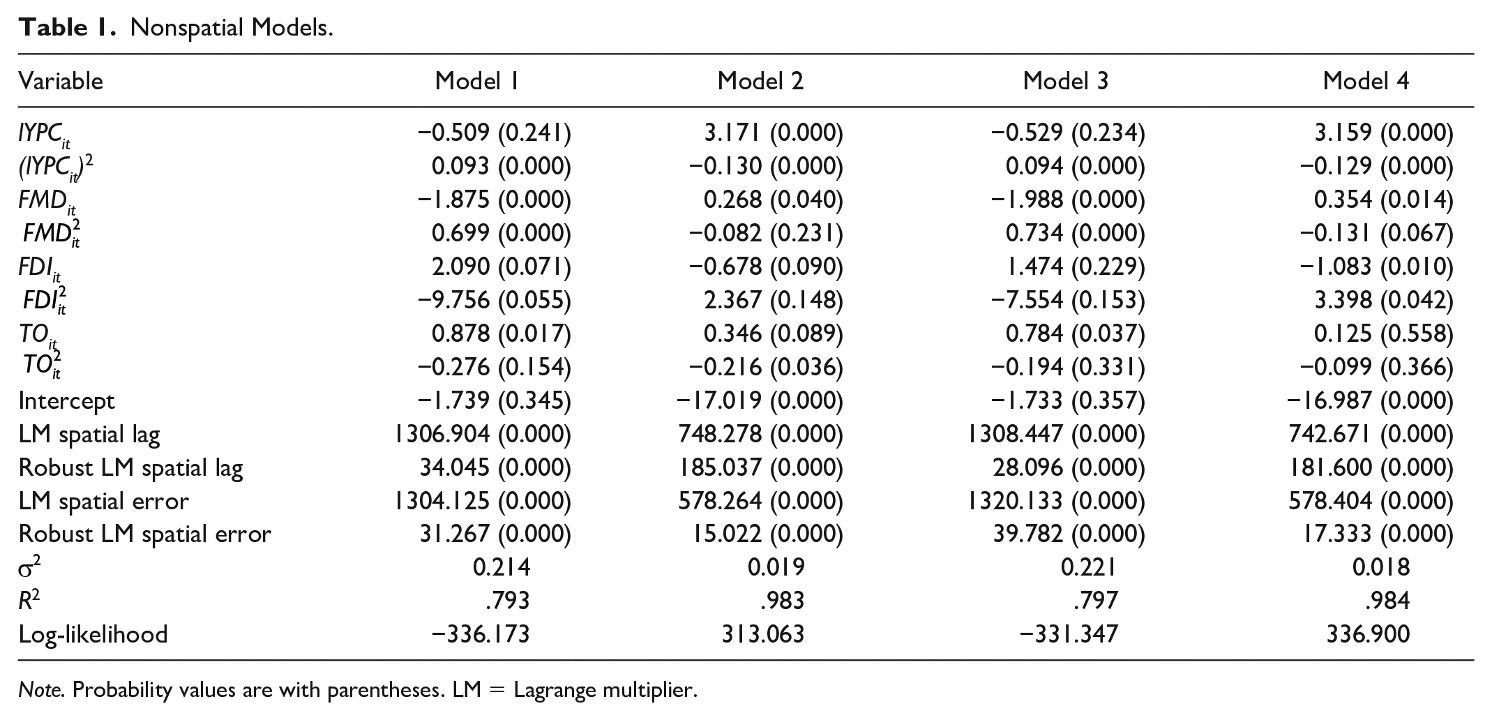
Note. Probability values are with parentheses. LM = Lagrange multiplier.

Table 1 also shows the results of LM and LM robust tests to verify the spatial effects in the models (1–4). Both tests are performed to verify the validity of spatial error and spatial lag models. The results showed that null hypothesis of nonspatial dependence has been rejected for all models (1–4). Therefore, we may confirm the spatial dependency in the estimated models and may conclude that spatial models are suitable and favorable over the nonspatial estimated models. After confirming the superiority of spatial models, we estimate an initial model assuming quadratic effect of only income variable through the SDM with both FE and random effects (RE) specifications.

The results of SDM are presented in Table 2. At first, we tested that SDM can be reduced to SAR or SEM. We regressed the SDM FE and SDM RE and applied the Wald test on the null hypotheses H₀₁: $γ = 0$ and H₀₂: $γ + δ ϕ = 0$ . Both hypotheses are rejected at 1% level for both SDM FE and SDM RE. For reconfirmation, we applied the LR test to compare SDM FE with SAR FE and SEM FE and SDM RE with SAR RE and SEM RE. The LR test validated the conclusions of the LM test. Hence, it can be said that both SDM FE and SDM RE are efficient and cannot be reduced to the spatial lag or spatial error models, and we can conclude that SDM estimations are most appropriate and best fit for the model. Furthermore, we applied the Hausman test with a null hypothesis “SDM RE model is a preferable model.” The result of the Hausman test, reported in the last row of Table 2, led to a rejection of the null hypothesis at 10% level of significance. Hence, we can conclude that SDM FE is preferable and better fit for estimations and this model can be chosen for further discussions.

Table 2.

Initial Model.

Variables	SDM FE				SDM RE
Variables	Point	Direct	Indirect	Total	Point	Direct	Indirect	Total
lYPC_it	3.518 (0.000)	3.557 (0.000)	−1.187 (0.000)	2.370 (0.000)	3.392 (0.000)	3.432 (0.000)	−1.185 (0.000)	2.247 (0.000)
(lYPC_it) ²	−0.155 (0.000)	−0.156 (0.000)	0.033 (0.017)	−0.123 (0.000)	−0.146 (0.000)	−0.148 (0.000)	0.031 (0.021)	−0.117 (0.000)
FMD_it	0.199 (0.000)	0.186 (0.000)	1.037 (0.000)	1.222 (0.000)	0.199 (0.000)	0.185 (0.001)	1.049 (0.000)	1.235 (0.000)
FDI_it	−0.465 (0.004)	−0.479 (0.003)	0.377 (0.388)	−0.101 (0.805)	−0.465 (0.005)	−0.480 (0.003)	0.469 (0.278)	−0.011 (0.978)
TO_it	0.071 (0.143)	0.059 (0.197)	0.759 (0.000)	0.818 (0.000)	0.068 (0.171)	0.056 (0.232)	0.736 (0.000)	0.792 (0.000)
W * lYPC_it	−0.535 (0.000)				−0.566 (0.000)
W * FMD_it	1.351 (0.000)				1.354 (0.000)
W * FDI_it	0.380 (0.467)				0.425 (0.424)
W * TO_it	0.941 (0.000)				0.918 (0.000)
W * lCO_it	−0.274 (0.024)				−0.272 (0.027)
R ²	.724				.730
$σ^{2}$	0.015 (0.000)				0.16 (0.027)
Log-likelihood	348.357				274.526
Spatial lag-LR test	77.82 (0.000)				74.20 (0.000)
Spatial error-LR test	78.21 (0.000)				75.12 (0.000)
Spatial lag-Wald test	84.15 (0.000)				80.24 (0.000)
Spatial error-Wald test	87.02 (0.000)				82.97 (0.000)
Hausman test	17.52 (0.064)

Note. Probability values are with parentheses. SDM = spatial Durbin model; FE = fixed effect; RE = random effect; LR = likelihood ratio.

The estimates of SDM FE showed that the coefficient of W*lCO_it is statistically significant and supports the existence of interdependence of CO₂ emissions per capita across the North American countries. Furthermore, the coefficients of W*lYPC_it, W*FMD_it, and W*TO_it are also statistically significant and showed spillover effects of such variables from neighboring countries on local CO₂ emissions per capita. Moreover, the estimated indirect effects may also be discussed for the spillover effects (LeSage & Pace, 2009). In the point, direct, and total estimates, the inverted U-shaped relationship has been found between the income per capita and CO₂ emissions per capita through positive (negative) coefficients of income (income square) variables. Therefore, we can conclude the existence of the EKC hypothesis for the panel of North American countries, while per capita income of neighboring countries has a U-shaped relationship with the local CO₂ emissions per capita in the indirect estimates. This U-shaped relationship in the indirect estimates is in line with nonspatial estimates of Martinez-Zarzoso and Bengochea-Morancho (2003) who conducted a panel of 19 Latin American countries, Dogan and Turkekul (2016) for the United States, Sapkota and Bastola (2017) for a panel of Latin American countries with income per capita lesser than US$3,550, and the spatial work of Maddison (2006) for a panel of 135 countries. This result corroborates that the rising income of neighboring countries puts pressure on local economy to control pollution.

The coefficients of FMD are positive and significant in all point, direct, indirect, and total estimates. Therefore, we may conclude that both local FMD and neighboring FMD have negative local environmental effects. Furthermore, scale effect of North American FMD is found dominant over technique and composition effects. This result also supports the idea of loans for consumption purpose in Latin American countries reported by de la Torre et al. (2012). Moreover, the indirect effect of FMD is found greater than the direct effect which is indicating that increasing FMD in neighboring countries even has greater negative environmental spillover effects on local CO₂ emissions per capita than the local adverse environmental effects of local FMD.

FDI has negative and significant effect on CO₂ emissions per capita in the point and direct estimates. Indirect and total effects of FDI and point and direct effects of trade openness are insignificant in the initial model’s estimates in Table 2 but statistically significant in the parsimonious model’s estimates mentioned in Table 4. Assuming the superiority of parsimonious estimates, it can be concluded that local FDI has pleasant environmental effects in the point, direct, and total estimates. The technique and/or composition effects of local FDI are dominant on the scale effect. Another conclusion that can be derived from this is that pollution haven and displacement hypotheses may be rejected in North America and foreign investors are promoting clean technologies which is in line with the arguments of Birdsall and Wheeler (1993) and Eskeland and Harrison (2003). On the contrary, the negative environmental spillover effects of neighboring countries’ FDI are recognized through indirect estimates. In the relationship of trade openness and CO₂ emissions per capita, all estimated coefficients are positive and significant and lead to the conclusion that trade openness of a country and its neighbors are positively contributing to the local CO₂ emissions per capita. Estimated negative environmental effect of trade openness in a panel of North America is in contrast to positive environmental effect of trade found by Dogan and Turkekul (2016) for the United States. Furthermore, the coefficient of trade openness in the indirect estimates is greater than that in direct estimates.

After estimation and discussion of the initial model, Table 3 presents the estimates of spatial SDM FE and SDM RE using a full model of Equation (5). The authenticity of SMD FE and SDM RE is verified by the Wald test and LR test. All tests suggest that SDM FE and SDM RE cannot be reduced to spatial lag or spatial error models. Furthermore, the Hausman test has confirmed the suitability of the SDM FE model. The results of the full model have been improved as the effect of trade openness has been turned to be significant in the point and direct estimates which was insignificant in the initial model. The fundamental purpose of regressing a full model is to test the possible existence of the inverted U-shaped relationship in all hypothesized variables. In the SDM FE results, the inverted U-shaped relationship has been found in case of income per capita and trade openness in the point, direct, and total estimates. An inverted U-shaped relationship between trade openness and CO₂ emissions per capita suggests that increasing trade openness has positive environmental effect after the turning point. In the indirect effects, income per capita has U-shaped effect, and both trade openness and its square term have positive effects on the local CO₂ emissions per capita. Furthermore, we found the monotonic positive (negative) effects of FMD (FDI) as their square terms have insignificant effects on all the estimates. Moreover, all spillover effects are significant through coefficients of weighted variables except W*FDI_it.

Table 3.

Full Model.

Variables	SDM FE				SDM RE
Variables	Point	Direct	Indirect	Total	Point	Direct	Indirect	Total
lYPC_it	3.456 (0.000)	3.498 (0.000)	−1.235 (0.000)	2.263 (0.000)	3.314 (0.000)	3.354 (0.000)	−1.207 (0.000)	2.147 (0.000)
(lYPC_it) ²	−0.150 (0.000)	−0.151 (0.000)	0.033 (0.008)	−0.118 (0.000)	−0.141 (0.000)	−0.142 (0.000)	0.030 (0.017)	−0.112 (0.000)
FMD_it	0.357 (0.005)	0.350 (0.005)	0.951 (0.000)	1.301 (0.000)	0.359 (0.005)	0.352 (0.005)	0.977 (0.000)	1.330 (0.000)
$F M D_{i t}^{2}$	−0.085 (0.186)	−0.090 (0.134)	0.020 (0.211)	−0.070 (0.139)	−0.088 (0.175)	−0.094 (0.123)	0.019 (0.195)	−0.074 (0.132)
FDI_it	−0.791 (0.035)	−0.813 (0.024)	0.484 (0.256)	−0.329 (0.497)	−0.766 (0.045)	−0.788 (0.032)	0.561 (0.225)	−0.227 (0.655)
$F D I_{i t}^{2}$	1.494 (0.323)	1.569 (0.292)	−0.340 (0.335)	1.228 (0.299)	1.366 (0.375)	1.440 (0.341)	−0.296 (0.407)	1.144 (0.343)
TO_it	0.520 (0.008)	0.508 (0.015)	0.622 (0.001)	1.130 (0.000)	0.508 (0.011)	0.497 (0.018)	0.609 (0.002)	1.106 (0.000)
$T O_{i t}^{2}$	−0.232 (0.020)	−0.233 (0.023)	0.052 (0.088)	−0.181 (0.024)	−0.228 (0.024)	−0.229 (0.027)	0.049 (0.111)	−0.180 (0.027)
W * lYPC_it	−0.586 (0.000)				−0.604 (0.000)
W * FMD_it	1.308 (0.000)				1.310 (0.000)
W * FDI_it	0.414 (0.424)				0.451 (0.393)
W * TO_it	0.916 (0.000)				0.901 (0.000)
W * lCO_it	−0.282 (0.022)				−0.280 (0.025)
R ²	.720				.725
$σ^{2}$	0.015 (0.000)				0.016 (0.000)
Log-likelihood	352.603				278.534
Spatial lag-LR test	75.11 (0.000)				72.03 (0.000)
Spatial error-LR test	77.07 (0.000)				74.97 (0.000)
Spatial lag-Wald test	80.99 (0.000)				77.65 (0.000)
Spatial error-Wald test	76.51 (0.000)				73.59 (0.000)
Hausman test	30.60 (0.004)

Note. Probability values are with parentheses. SDM = spatial Durbin model; FE = fixed effect; RE = random effect; LR = likelihood ratio.

A parsimonious model is estimated and presented in Table 4, after removing all the insignificant effects of $F M D_{i t}^{2}$ , $F D I_{i t}^{2}$ , and W*FDI_it from the full model in Table 3. The purpose of the parsimonious model is to estimate the reliable magnitudes of coefficients to conclude the results. At first, parsimonious model is estimated by SDM FE and SDM RE. Then, the Wald test and LR test were used to see whether SDM estimates can be reduced to spatial lag and special error models. Both the Wald test and LR test rejected the null hypotheses H₀₁: $γ = 0$ and H₀₂: $γ + δ ϕ = 0$ and corroborated that SDM FE and SDM RE cannot be reduced to SAR or SEM. Hence, SDM is most efficient in the parsimonious model. Furthermore, the Hausman test is applied and it rejected the null hypothesis of “SDM RE is the preferable model,” which indicated that SDM FE estimates are a better fit for the analysis. All estimated coefficients of the parsimonious model through SDM FE are statistically significant and may be considered to be more efficient to discuss the magnitudes of effects compared with those of previous estimated models in Tables 2 and 3. The statistically significant coefficients of weighted variables are showing significant spillover effects of CO₂ emissions per capita, per capita income, FMD, and trade openness from neighboring countries on the local CO₂ emissions per capita.

Table 4.

Parsimonious Model.

Variables	SDM FE				SDM RE
Variables	Point	Direct	Indirect	Total	Point	Direct	Indirect	Total
lYPC_it	3.558 (0.000)	3.599 (0.000)	−1.223 (0.000)	2.376 (0.000)	3.422 (0.000)	3.463 (0.000)	−1.219 (0.000)	2.244 (0.000)
(lYPC_it) ²	−0.156 (0.000)	−0.157 (0.000)	0.034 (0.011)	−0.123 (0.000)	−0.147 (0.000)	−0.149 (0.000)	0.033 (0.007)	−0.116 (0.000)
FMD_it	0.199 (0.000)	0.185 (0.000)	1.003 (0.000)	1.188 (0.000)	0.197 (0.000)	0.183 (0.001)	1.013 (0.000)	1.196 (0.000)
FDI_it	−0.415 (0.010)	−0.422 (0.007)	0.093 (0.068)	−0.329 (0.009)	−0.415 (0.012)	−0.422 (0.008)	0.094 (0.049)	−0.329 (0.011)
TO_it	0.544 (0.006)	0.533 (0.006)	0.680 (0.000)	1.213 (0.000)	0.532 (0.007)	0.521 (0.008)	0.661 (0.000)	1.182 (0.000)
$T O_{i t}^{2}$	−0.243 (0.015)	−0.242 (0.014)	0.053 (0.082)	−0.189 (0.017)	−0.238 (0.018)	−0.238 (0.017)	0.053 (0.072)	−0.185 (0.020)
W * lYPC_it	−0.537 (0.000)				−0.557 (0.000)
W * FMD_it	1.314 (0.000)				1.316 (0.000)
W * TO_it	0.982 (0.000)				0.970 (0.000)
W * lCO_it	−0.288 (0.015)				−0.283 (0.018)
R ²	.718				.724
$σ^{2}$	0.015 (0.000)				0.016 (0.000)
Log-likelihood	351.057				276.991
Spatial lag-LR test	74.99 (0.000)				71.71 (0.000)
Spatial error-LR test	74.94 (0.000)				73.06 (0.000)
Spatial lag-Wald test	80.85 (0.000)				77.31 (0.000)
Spatial error-Wald test	79.55 (0.000)				76.32 (0.000)
Hausman test	34.81 (0.000)

Note. Probability values are with parentheses. SDM = spatial Durbin model; FE = fixed effect; RE = random effect; LR = likelihood ratio.

The EKC hypothesis is corroborated in North America with positive (negative) coefficients of lYPC_it (lYPC_it)² in the point, direct, and total estimates. It corroborates that a lower level of income carries negative environmental effects, and CO₂ emissions reduce at a higher level of income. The economic growth of such countries is helpful in protecting the environment by reducing CO₂ emissions. Furthermore, the turning point of the inverted U-shaped relationship is found at approximately 89,666 constant (2010) U.S. dollar per capita GDP in the point estimates (exponent of 3.558/0.156/2). This turning point is out of range of per capita income of all sample countries and may be supposed biased because spillover effects from neighboring countries were ignored. Considering both direct and indirect effects, the turning point is calculated at approximately 15,655 per capita GDP from the total effects’ estimates (exponent of 2.376/0.123/2). This turning point has been achieved by 6 of the 21 sample North American countries. Bahamas, Canada and the United States have achieved this turning point before 1990, a starting year of our sample period. However, Barbados, St. Kitts and Nevis, and Trinidad and Tobago have achieved the turning point at the years 2005, 2016, and 2006, respectively. Therefore, it can be concluded that 6 of the 21 sample countries are on the second phase of the EKC, and economic growth of such countries is helpful in protecting environment by reducing CO₂ emissions. We may also conclude that 15 of the 21 countries are still on the economic growth policy without caring environmental degradation. With some mathematical application, we may also conclude the inelastic impact of GDP per capita on the per capita CO₂ emissions in the total estimates during the sample period. Hence, keeping other variables constant, per capita CO₂ emission is increasing less than 1% with 1% increase in GDP per capita. The indirect effect of economic growth is found to be U-shaped, and this result is in line with the findings of nonspatial conclusions of Martinez-Zarzoso and Bengochea-Morancho (2003) in case of 19 Latin American countries, Dogan and Turkekul (2016) in case of the United States, and Sapkota and Bastola (2017) in case of low-income Latin American countries and is also in line with the spatial results of Maddison (2006) in case of a large panel of 135 countries. This result validates that the economic growth of a country in the North American region puts pressure on the neighboring countries to reduce CO₂ emissions.

Trade openness has an inverted U-shaped relationship with per capita CO₂ emissions in the point, direct, and total estimates. In the indirect effect, the coefficients of trade openness and its square term are positive and show adverse spillover environmental effects. Furthermore, these negative spillover environmental effects of neighboring countries’ trade openness are found more extensive than the local trade openness direct effect. In the total effect of trade openness, the turning point of the inverted U-shaped relationship is estimated at the trade-to-GDP ratio = 3.209% or 320.9% (1.213/0.189/2). Trade openness of all sample North American countries is less than the 3.209 ratio. Therefore, we may conclude that all countries are on the first phase of the inverted U-shaped relationship, and trade openness is responsible for negative environmental effects. Furthermore, elasticity of trade openness may be estimated as greater than one in the sample period. The negative environmental effect of trade shows pollution-oriented trade in this region as per the arguments of Liddle (2001). Moreover, Dogan and Turkekul found positive environmental impacts of trade in the United States. But the net negative ecological effect of trade in the whole North American region implies the displacement hypothesis in this region as per the arguments of Copeland and Taylor (1995).

FMD has a positive contribution to the CO₂ emissions per capita in all estimated effects. So, the scale effects of FMD are found more substantial than the possible technique and composition effects of FMD. This result also confirms the arguments of de la Torre et al. (2012) that financial markets of Latin American countries have promoted loans for consumption purposes. Furthermore, the indirect effect of FMD is found higher than the direct effect. It means that FMD of a country has negative spillovers on the neighboring countries more significantly than the direct impact on the domestic environment. FDI has negative and significant effects on CO₂ emissions per capita in the point, direct, and total estimates. This result implies that the technique and composition effects of FDI are found dominant on the scale effect. It means foreign investors have better environmental standards in production and resultantly have positive environmental effects through using cleaner technology, as argued by Birdsall and Wheeler (1993) and Eskeland and Harrison (2003). Furthermore, the PHH of foreign investment is not proved in the North American region. But FDI has negative environmental spillover effect on the indirect estimates, and a unit increase in FDI inflows in neighboring countries is responsible for 9.3% increase in local CO₂ emissions per capita.

Conclusion

This study attempted to test the impact of income per capita, FMD, FDI, and trade openness on the per capita CO₂ emissions for a panel of 21 North American countries from 1990 to 2014. Spatial dependency is found in the estimated nonspatial CO₂ emissions’ models. An appropriateness of SDM has also been tested and found over SAR and SEM. Furthermore, the hypothesized model has been estimated through SDM in the three stages to approach a parsimonious model for unbiased estimates. At first, a model is estimated to test the EKC hypothesis in the nonlinear relationship between income per capita and CO₂ emissions per capita along with linear effects of FMD, trade openness, and FDI. Second, another model is estimated by assuming nonlinear effects of all hypothesized variables. Finally, a parsimonious model is chosen by removing insignificant effects from a full model.

An inverted U-shaped relationship is found between GDP per capita and CO₂ emissions per capita. Furthermore, the turning point of GDP per capita effect is found at $15,655 U.S. constant dollars. The estimated turning point suggested that the United States, Canada, Bahamas, Barbados, St. Kittes and Nevis, and Trinidad and Tobago are found at the second stage of the EKC, and the rest of the 15 countries are still on the first phase. We can conclude that economic growth of 6 of the 21 investigated North American countries is helping to reduce CO₂ emissions, but CO₂ emissions are rising with economic growth in the rest of the countries.

Trade openness and CO₂ emissions per capita have inverted U-shaped relationship, and all sample countries are in the first phase of this inverted U-shaped relationship. Hence, the study leads to an inference that trade openness of the North American region is responsible for environmental degradation. Furthermore, spillover effects of trade openness are found greater than the direct impact of local trade openness. Local and neighboring FMD are responsible for increasing CO₂ emissions per capita, while spillover effects seem larger than the local direct effects. Finally, local FDI is helping to reduce CO₂ emissions per capita, but spillover effects from neighboring countries’ FDI are responsible for environmental degradation.

Based on the result of harmful environmental effects of FMD, we recommend the North American countries to put qualitative checks in the financial market by offering the renewable energy credit to the investors who put their loans in the renewable energy projects and to tax the investment in the nonrenewable projects. Better financing schemes for carbon capture, energy storage, and clean coal technologies are required for these North American countries to improve their ecological footprint. Trade openness is also found responsible for environmental degradation. So, the imports of energy consumption–oriented products should have higher taxes and exports from the dirty industry should also be discouraged. Finally, the FDI has pleasant environmental effects and technological change through foreign investment can help to reduce the negative impact of high emissions. So, foreign investors should be attracted by offering tax holidays for their investment and renewable energy credit may also be offered for foreign investment in the renewable energy projects. Last but not least, the pollution spillovers should not be ignored while designing trade, investment, and growth policies.

Footnotes

Declaration of Conflicting Interests

The author(s) declared no potential conflicts of interest with respect to the research, authorship, and/or publication of this article.

Funding

The author(s) received no financial support for the research, authorship, and/or publication of this article.

ORCID iD

Haider Mahmood

References

Acaravci

Akalin

(2017). Environment–economic growth nexus: A comparative analysis of developed and developing countries. International Journal of Energy Economics and Policy, 7(5), 34–43.

Ajmi

A. N.

Hammaoudeh

Nguyen

D. K.

Sato

J. R.

(2015). On the relationships between CO2 emissions, energy consumption and income: The importance of time variation. Energy Economics, 49, 629–638.

Aldy

J. E.

(2005). An environmental Kuznets curve analysis of U.S. state-level carbon dioxide emissions. The Journal of Environment & Development, 14, 48–72.

Alola

A. A.

(2019). The trilemma of trade, monetary and immigration policies in the United States: Accounting for environmental sustainability. Science of the Total Environment, 658, 260–267.

Ameyaw

Yao

Oppong

Agyeman

(2019). Investigating, forecasting and proposing emission mitigation pathways for CO2 emissions from fossil fuel combustion only: A case study of selected countries. Energy Policy, 130(1), 7–21.

Anastacio

J. A. R.

(2017). Economic growth, CO2 emissions and electric consumption: Is there an Environmental Kuznets Curve? An empirical study for North America countries. International Journal of Energy Economics and Policy, 7(2), 65–71.

Anselin

(1988). Spatial econometrics: Methods and models. Springer.

Anselin

Le Gallo

Jayet

(2008). Spatial panel econometrics. In Matyas

Sevestre

(Eds.), The econometrics of panel data (pp. 625–660). Springer.

Antweiler

Copeland

B. R.

Taylor

M. S.

(2001). Is free trade good for the environment? American Economic Review, 91(4), 877–908.

10.

Apergis

Christoua

Guptab

(2017). Are there environmental Kuznets curves for U.S. state-level CO2 emissions? Renewable and Sustainable Energy Reviews, 69, 551–558.

11.

Apergis

Ozturk

(2015). Testing the environmental Kuznets curve hypothesis in Asian countries. Ecological Indicators, 52, 16–22.

12.

Arrow

Bolin

Costanza

Folke

Holling

C. S.

Janson

Levin

Maler

Perrings

Pimental

(1995). Economic growth, carrying capacity, and the environment. Science, 15, 91–95.

13.

Aslan

Destek

M. A.

Okumus

(2018). Bootstrap rolling window estimation approach to analysis of the Environment Kuznets Curve hypothesis: Evidence from the USA. Environmental Science and Pollution Research, 25(3), 2402–2408.

14.

Atasoy

B. S.

(2017). Testing the environmental Kuznets curve hypothesis across the U.S.: Evidence from panel mean group estimators. Renewable and Sustainable Energy Reviews, 77, 731–747.

15.

Auffhammer

Steinhauser

(2007). The future trajectory of U.S. CO2 emissions: The role of state vs. aggregate information. Journal of Regional Science, 47(1), 47–61.

16.

Balshi

M. S.

Mcguire

A. D.

Duffy

Flannigan

Kicklighter

D. W.

(2009). Vulnerability of carbon storage in North American boreal forests to wildfires during the 21st century. Global Change Biology, 15, 1491–1510.

17.

Bhattarai

Hammig

(2001). Institutions and the environmental Kuznets curve for deforestation: A crosscountry analysis for Latin America, Africa and Asia. World Development, 29(6), 995–1010.

18.

Birdsall

Wheeler

(1993). Trade policy and industrial pollution in Latin America: Where are the pollution havens? The Journal of Environment & Development, 2, 137–149.

19.

Blanco

Gonzalez

Ruiz

(2013). The impact of FDI on CO2 emissions in Latin America. Oxford Development Studies, 41(1), 104–121.

20.

Bockstael

N. E.

(1996). Modeling economics and ecology: The importance of a spatial perspective. American Journal of Agricultural Economics, 78, 1168–1180.

21.

Burnett

J. W.

Bergstrom

J. C.

Dorfman

J. H.

(2013). A spatial panel data approach to estimating U.S. state-level energy emissions. Energy Economics, 40, 396–404.

22.

Burnett

J. W.

Bergstrom

J. C.

Wetzstein

M. E.

(2013). Carbon dioxide emissions and economic growth in the U.S. Journal of Policy Modeling, 35(6), 1014–1028.

23.

Carson

R. T.

Jeon

McCubbin

(1997). The relationship between air pollution emissions and income: U.S. data. Environment and Development Economics, 2, 433–450.

24.

Cherniwchan

(2017). Trade liberalization and the environment: Evidence from NAFTA and U.S. manufacturing. Journal of International Economics, 105, 130–149.

25.

Congregado

Feria-Gallardo

Golpe

A. A.

Iglesias

(2016). The environmental Kuznets curve and CO2 emissions in the USA: Is the relationship between GDP and CO2 emissions time varying? Evidence across economic sectors. Environmental Science and Pollution Research, 23, 18407–18420.

26.

Copeland

B. R.

Taylor

M. S.

(1995). Trade and the environment: A partial synthesis. American Journal of Agricultural Economics, 77, 765–771.

27.

Debarsy

Ertur

(2010). Testing for spatial autocorrelation in a fixed effects panel date model. Regional Science and Urban Economics, 40, 453–470.

28.

de Knegt

H. J.

Coughenour

M. B.

Skidmore

A. K.

Heitkonig

I. M. A.

Know

N. M.

Slotow

Prins

H. H. T

. (2010). Spatial autocorrelation and the scaling of species-environment relationships. Ecology, 91(8), 2455–2465.

29.

de la Torre

Ize

Schmukler

S. L.

(2012). Financial development in Latin America and the Caribbean: The road ahead. The World Bank.

30.

Dinda

(2004). Environmental Kuznets curve hypothesis: A survey. Ecological Economics, 49, 431–455.

31.

Dogan

Turkekul

(2016). CO2 emissions, real output, energy consumption, trade, urbanization and financial development: Testing the EKC hypothesis for the USA. Environmental Science and Pollution Research, 23(2), 1203–1213.

32.

Elhorst

J. P.

(2001). Dynamic models in space and time. Geographical Analysis, 33(2), 119–140.

33.

Elhorst

J. P.

(2010). Spatial panel data models. In Fischer

M. M.

Getis

(Eds.), Handbook of applied spatial analysis (pp. 377–407). Springer.

34.

Elhorst

J. P.

(2012). Matlab software for spatial panels. International Regional Science Review, 35(4), 1–17.

35.

Energy Information Administration. (2019). Online database. https://www.eia.gov/

36.

Eskeland

G. S.

Harrison

A. E.

(2003). Moving to greener pastures? Multinationals and the pollution haven hypothesis. Journal of Development Economics, 70(1), 1–23.

37.

Essandoh

Islam

Kakinaka

(2020). Linking international trade and foreign direct investment to CO2 emissions: Any differences between developed and developing countries? Science of the Total Environment, 712, 136437.

38.

Frankel

J. A.

Romer

(1999). Does trade cause growth? American Economic Review, 89(3), 379–399.

39.

Gale

L. R.

IV . (1995). Trade liberalization and pollution: An input-output study of carbon dioxide emissions in Mexico. Economic Systems Research, 7(3), 309–320.

40.

Gregg

J. S.

Losely

L. M.

Andres

R. J.

Blasing

T. J.

Marland

(2009). The temporal and spatial distribution of carbon dioxide emissions from fossil-fuel use in North America. Journal of Applied Meteorology and Climatology, 48, 2528–2542.

41.

Grossman

G. M.

Krueger

A. B.

(1991, November). Envi-ronmental impacts of the North American free trade agreement (NBER Working Paper No. 3914). https://www.nber.org/papers/w3914

42.

Grossman

G. M.

Krueger

A. B.

(1995). Economic growth and the environment. The Quarterly Journal of Economics, 110(2), 353–377.

43.

Grossman

G. M.

Krueger

A. B.

(1996). The inverted-U: What does it mean? Environment and Development Economics, 1(1), 119–122.

44.

Guevara

Molina-Perez

Garcia

E. X. M.

Perez-Cirera

(2019). Energy and CO2 emission relationships in the NAFTA trading bloc: A multi-regional multi-factor energy input–output approach. Economic System Research, 31(2), 178–205.

45.

Henriques

S. T.

Borowiecki

K. J.

(2017). The drivers of long-run CO2 emissions in Europe, North America and Japan since 1800. Energy Policy, 101, 537–549.

46.

Kelejian

Prucha

(2010). Specification and estimation of spatial autoregressive models with autoregressive and heteroskedastic disturbances. Journal of Econometrics, 157(1), 53–67.

47.

Kerr

Mellon

(2012). Energy, population and the environment: Exploring Canada’s record on CO2 emissions and energy use relative to other OECD countries. Population and Environment, 34(2), 257–278.

48.

Komen

Gerking

Folmer

(1997). Income and environmental R&D: Empirical evidence from OECD countries. Environment and Development Economics, 2, 505–515.

49.

Kuznets

(1955). Economic growth and income inequality. American Economic Review, 45(1), 1–28.

50.

Lankao

P. R.

(2004). Pathways regional development and the carbon cycle. In Field

C. B.

Raupach

M. R.

(Eds.), The global carbon cycle: Integrating human, climate, and the natural world (pp. 355–369). Island Press.

51.

Lantz

Feng

(2006). Assessing income, population, and technology impacts on CO2 emissions in Canada: Where’s the EKC? Ecological Economics, 57, 229–238.

52.

LeSage

J. P.

Pace

R. K.

(2009). An introduction to spatial econometrics. CRC Press.

53.

Liddle

(2001). Free trade and the environment-development system. Ecological Economics, 39(1), 21–36.

54.

Lipford

J. W.

Yandle

(2011). NAFTA, environmental Kuznets curves, and Mexico’s progress. Global Economy Journal, 10(4), 1850211.

55.

Maddison

(2006). Environmental Kuznets curves: A spatial econometric approach. Journal of Environmental Economics and Management, 51, 218–230.

56.

Mahmood

Alrasheed

A. S.

Furqan

(2018). Financial market development and pollution nexus in Saudi Arabia: Asymmetrical analysis. Energies, 11(12), 3462.

57.

Mahmood

Furqan

Bagais

O. A.

(2019). Environmental accounting of financial development and foreign investment: Spatial analyses of East Asia. Sustainability, 11(1), 13.

58.

Martinez-Zarzoso

Bengochea-Morancho

(2003). Testing for an environmental Kuznets curve in Latin-American countries. Economic Analysis Review, 18(1), 3–26.

59.

Olale

Ochuodho

T. O.

Lantz

El Armali

(2018). The environmental Kuznets curve model for greenhouse gas emissions in Canada. Journal of Cleaner Production, 184, 859–868.

60.

Ozturk

Acaravci

(2013). The long-run and causal analysis of energy, growth, openness and financial development on carbon emissions in Turkey. Energy Economics, 36, 262–267.

61.

Panayotou

(1993). Empirical tests and policy analysis of environmental degradation at different stages of economic development. Technology and Employment Programme, International Labour Organization. https://econpapers.repec.org/paper/iloilowps/992927783402676.htm

62.

Pata

U. K.

(2018). The influence of coal and noncarbohydrate energy consumption on CO2 emissions: Revisiting the environmental Kuznets curve hypothesis for Turkey. Energy, 160, 1115–1123.

63.

Pataki

D. E.

Alig

R. J.

Fung

A. S.

Golubiewski

N. E.

Kennedy

C. A.

McPherson

E. G.

Nowak

D. J.

Pouyat

R. V.

Lankao

P. R.

(2006). Urban ecosystems and the North American carbon cycle. Global Change Biology, 12, 1–11.

64.

Pazienza

(2019). The impact of FDI in the OECD manufacturing sector on CO2 emission: Evidence and policy issues. Environmental Impact Assessment Review, 77(1), 60–68.

65.

Poudel

B. N.

Paudel

K. P.

Bhattarai

(2009). Searching for an environmental Kuznets curve in carbon dioxide pollutant in Latin American countries. Journal of Agricultural and Applied Economics, 41, 13–27.

66.

Rupasingha

Geotz

S. J.

Debertin

D. L.

Pagoulatos

(2004). The environmental Kuznets curve for U.S. counties: A spatial econometric analysis with extensions. Papers in Regional Science, 83, 407–424.

67.

Sapkota

Bastola

(2017). Foreign direct investment, income, and environmental pollution in developing countries: Panel data analysis of Latin America. Energy Economics, 64, 206–212.

68.

Selden

T. M.

Song

(1994). Environmental quality and development: Is there a Kuznets curve for air pollution emissions? Journal of Environmental Economics and Management, 27(2), 147–162.

69.

Shafik

Bandyopadhyay

(1992, June). Economic growth and environmental quality: Time series and cross-country evidence (World Bank Working Papers, WPS 904). https://documents.worldbank.org/en/publication/documents-reports/documentdetail/833431468739515725/economic-growth-and-environmental-quality-time-series-and-cross-country-evidence

70.

Shahbaz

Gozgor

Adom

Hammoudeh

(2019). The technical decomposition of carbon emissions and the concerns about FDI and trade openness effects in the United States. International Economics, 159(1), 56–73.

71.

Shahbaz

Solarin

S. A.

Sbia

Bibi

(2015). Does energy intensity contribute to CO2 emissions? A trivariate analysis in selected African countries. Ecological Indicators, 50, 215–224.

72.

Soytas

Sari

Ewing

B. T.

(2007). Energy consumption, income, and carbon emissions in the United States. Ecological Economics, 62, 482–489.

73.

Tai

Chao

C. C.

S. W.

(2015). Pollution, health and economic growth. The North American Journal of Economics and Finance, 32, 155–161.

74.

Ulucak

Yücel

A. G.

Koçak

(2019). The process of sustainability: From past to present. In Ozcan

Ozturk

(Eds.), Environmental Kuznets Curve (EKC): A manual (pp. 37–53). Academic Press.

75.

Union of Concerned Scientists. (2019). Each country’s share of CO2 emissions. https://www.ucsusa.org/resources/each-countrys-share-co2-emissions

76.

Vukina

Beghin

J. C.

Solakoglu

E. G.

(1999). Transition to markets and the environment: Effects of the change in the composition of manufacturing output. Environment and Development Economics, 4(4), 582–598.

77.

Waldkirch

Gopinath

(2008). Pollution control and foreign direct investment in Mexico: An industry-level analysis. Environmental and Resource Economics, 41(3), 289–313.

78.

Wang

Kang

L. Y.

X. Q.

Xiao

(2013). Estimating the environmental Kuznets curve for ecological footprint at the global level: A spatial econometric approach. Ecological Indicators, 34, 15–21.

79.

The World Bank. (2019). World development indicators.

80.

Zhang

Y. J.

(2011). The impact of financial development on carbon emissions: An empirical analysis in China. Energy Policy, 39(4), 2197–2203.

CO 2 Emissions,Financial Development,Trade,and Income in North America: A Spatial Panel Data Approach

Abstract

Keywords

Introduction

Literature Review

Theoretical Background

Method

Data Analyses and Discussions

Conclusion

Footnotes

Declaration of Conflicting Interests

Funding

ORCID iD

References