Sage Journals: Discover world-class research

Abstract

This study examines the impact of environmental and non-environmental goods trade on environmental quality in OECD countries over the period 1995 to 2021. Using the Quantile Regression for Panel Data (QRPD) method, the analysis explores how these two types of trade influence the Environmental Performance Index (EPI) across countries with varying levels of environmental quality. The key explanatory variables include trade in environmental goods, trade in non-environmental goods, economic growth and its squared term (to test the Environmental Kuznets Curve [EKC] hypothesis), and urbanization. The findings indicate that trade in environmental goods enhances environmental quality. In contrast, trade in non-environmental goods generally has a detrimental effect, particularly in countries with low to medium levels of environmental performance. Economic growth is associated with environmental degradation, while its squared term has a positive effect, supporting the validity of the EKC hypothesis. Urbanization is found to negatively affect environmental quality across all levels. The results also suggest that limiting the export of non-environmental goods and promoting the import of environmental goods may contribute to environmental improvement. By disaggregating trade effects and employing a distribution-sensitive method, the study provides novel empirical evidence. It offers policy-relevant insights and encourages the formulation of environmentally responsive trade and development strategies aligned with sustainable growth objectives.

Plain Language Summary

How Trade in Environmental and Non-Environmental Goods Affects the Environment in OECD Countries

The present study investigates the effect of international trade on environmental quality in OECD countries. A distinction is made between two categories of trade: environmental goods (including renewable energy equipment and pollution control technologies) and non-environmental goods (comprising traditional resource-intensive products). The findings of the present study demonstrate that: The trade in environmental goods has been demonstrated to engender improvements in environmental quality, particularly in countries exhibiting low or medium environmental performance levels. The dissemination of these goods is accompanied by the propagation of cleaner technologies and the promotion of sustainable practices. The trade of non-environmental goods has been demonstrated to have a detrimental effect on environmental quality, with the most significant negative impacts being observed in countries experiencing challenges related to pollution. The initial phase of economic growth is characterised by a deterioration in environmental quality. However, as income levels rise, environmental conditions undergo a positive transformation, a phenomenon that aligns with the findings of the Environmental Kuznets Curve (EKC). Urbanisation has been demonstrated to have a detrimental effect on environmental quality in all countries, although its negative impact is less significant in countries that have more stringent environmental standards. The present study employs a novel approach that separates environmental and non-environmental goods, utilising a method that captures differences across countries. This methodological innovation offers novel insights into the trade–environment relationship. The findings indicate that policies promoting the trade of environmental goods and restricting the trade of harmful goods can assist countries in achieving objectives related to cleaner growth and sustainability.

Keywords

environmental quality environmental goods trade non-environmental goods trade environmental Kuznets curve hypothesis quantile regression for panel data

Introduction

For decades, international trade has been seen as an important factor of economic growth by enabling countries to produce goods and services according to their comparative advantage. However, the impact of trade on climate remains a matter of debate. With increasing evidence of the climate crisis, the pollution of ecosystems, and declining biodiversity, global threats to environmental sustainability have begun to arise. Multilateral agreements on environmental issues like the Sustainable Development Goals (SDGs) and the Paris Climate Agreement have influenced numerous economic and political decisions, including trade. Despite the little advancement in this direction, environmental challenges have increasingly become part of the trade agenda, particularly in the expanding context of sustainability debates (Sauvage, 2014). The Doha Round of the World Trade Organization (WTO) addressed the trade liberalization of environmental goods and negotiations were held to lower tariff and non-tariff barriers to these goods (UNEP, 2013). It was multilateral negotiations among a group of WTO members on the Environmental Goods Agreement (EGA) aimed at fostering trade in certain key environmental products, like wind turbines and solar panels. They sought to eliminate tariffs on trade in environmental goods (EG), covering a wide range of goods used to produce renewable energy, which help prevent, control and reduce pollution, manage and conserve natural resources and monitor the environment. The 18th and final round of the discussions was held in Geneva from November 26 to December 2, 2016. The participants negotiated the EGA in terms of product coverage and various configurations. The constructive discussions led to renewed commitments to finalizing the EGA. The participants constituted most of the global trade in environmental goods (WTO, 2014; Zugravu-Soilita, 2019).

There is currently no common, internationally accepted list of these environmental goods and services, so many goods can be included in this scope, which makes classification difficult. With the advances in technology, the differences between environmental and non-environmental goods have become another issue. Besides, including both intermediate and finished goods on this list creates other problems regarding classification. Moreover, the multiple uses of some goods make classification even more difficult. Despite these hardships, there are some internationally used lists like the Friends Group, PEGS, APEC, CLEG Core, and CLEG Core+ (Sauvage, 2014). In 1995, the OECD/Eurostat Informal Working Group convened in Luxembourg to come to an agreement that the development of products and services geared toward measuring, stopping, limiting, reducing, or correcting damage to water, air, and soil, as well as harm caused by waste, noise, and ecosystem challenges, make up the environmental goods and services sector. Furthermore, these initiatives include resources, products, and technologies that reduce environmental threats, as well as decreasing air pollution and resource consumption (Steenblik, 2005).

International trade can influence environmental quality through multiple channels, including scale, composition, technique and transportation. However, the extant evidence remains equivocal when aggregate trade measures (total exports, imports, trade openness) are employed (Antweiler et al., 2001; Grossman & Krueger, 1991). One of the important decisions taken on trade in environmental goods during the WTO’s Doha Round was to address the liberalization of trade in environmental goods and to hold negotiations on reducing customs duties and non-tariff barriers applied to these goods (UNEP, 2013).

The present study adopts the IMF list as a point of reference, eschewing the use of alternative classifications such as those proposed by APEC or OECD/CLEG. The IMF list is distinguished by its comprehensive coverage of contemporary clean-tech supply chains, encompassing both conventional environmental-protection goods and adapted products (e.g., biofuels, hybrid vehicles). This breadth is crucial for decomposing EG and non-EG trade in OECD economies, where much of the environmental improvement is driven by technology diffusion embodied in traded goods (IMF, 2021).

The Environmental Performance Index (EPI, 0–100) is utilized as a multidimensional benchmark for evaluating environmental outcomes. The Environmental Performance Index (EPI) is a composite index that ranks countries based on their environmental sustainability performance. The EPI assesses the status of 180 countries across 58 indicators in 11 subject categories, including climate change, environmental health, and ecosystem vitality. In addition to indicating the proximity of countries to achieving established environmental policy targets, the index provides policymakers with direction on problem identification, target-setting, trend monitoring and best practices sharing. Consequently, the EPI is crucial for formulating approaches for sustainable development by rendering environmental successes and failures easily observable (Block et al., 2024).

The current research utilized the Environmental Performance Index (EPI) as a proxy for environmental quality. The EPI is a broad metric that measures environmental performance along a wide range of dimensions, using a diverse array of indicators. In addition, using EPI in assessing environmental quality is very useful for understanding current environmental situation and also for taking necessary strategic steps towards sustainability goal. It will help to fill an important gap, as it will treat environmental and non-environmental goods separately and will put special emphasis on the OECD countries. We must be able to see selected quantitative analysis conducted on cross countries empirical based ESG data thrust imports. This study also the impact of trade gains or loss for selected environmental quality at a country level.

As demonstrated in seminal studies such as those by Zugravu-Soilita (2018, 2019), trade has been decomposed into its environmental and non-environmental components, thus providing significant insights into the trade–environment nexus. Building on this literature, the present study contributes to the extant literature by employing the IMF classification that includes “adapted products,” utilizing the Environmental Performance Index (EPI) as a broader measure of environmental quality beyond CO₂ emissions, and by applying a quantile regression framework for panel data that captures heterogeneity across OECD countries (Figure 1).

Figure 1.

Impact pathways of trade on environmental performance index.

The five main economic and environmental pathways through which EG Trade Volume and NEG Trade Volume affect the Environmental Performance Index (EPI) are illustrated in the figure above. Green indicates positive environmental impact, red indicates negative impact and grey indicates neutral or mixed impact depending on the specific trade conditions. Compared to the volume of trade in emission-producing goods (NEG Trade Volume), EG Trade Volume is usually accompanied by an improvement in environmental performance due to positive technical and composition effects and negative scale and transport effects, respectively. The net impact of trade on environmental performance will be determined by the respective magnitudes of sectoral international trade flows and the nature of the policy response on civil issues related to pollution-intensive services. This study investigates how trade in environmental and non-environmental goods and services affects environmental quality among OECD countries using the Quantile Regression for Panel Data (QRPD) method. QRPD is particularly suitable for the objectives of this study as it captures cross-country heterogeneity and allows the analysis of distributional effects across different quantiles, rather than focusing only on average impacts. QRPD is particularly suitable for the objectives of this study as it captures cross-country heterogeneity and allows the analysis of distributional effects across different quantiles, rather than focusing only on average impacts. In addition, QRPD provides consistent estimates even when the time dimension is relatively short, which makes it especially appropriate for OECD panel data covering a limited time span. Moreover, while the environmental consequences of trade have been analyzed in the literature primarily from the perspective of trade volume, only a few papers deal with the environmental and non-environmental parts of trade separately. The theory underlying this research is that the effects of trade on environmental and non-environmental products can and should be decomposed. In this context, considering that trade can have positive effects on trade in environmental goods and negative effects on trade in non-environmental goods, it is theoretically argued that the effects of trade on environmental quality may vary depending on the type of goods and this relationship is supported by the results of empirical analyses in order to fill the gap in the literature. In this context, the effects of trade on the environment at five different environmental quality levels are analyzed in depth with the QRPD method and it is examined how these effects are not consistent across countries.

The present study poses the following research problem: The central research question guiding this study is whether trade in environmental goods, as classified by the IMF, enhances multidimensional environmental quality (EPI) across OECD countries in comparison to non-environmental trade. This inquiry encompasses two key aspects: firstly, the investigation of how these effects vary across the distribution of environmental performance, utilizing the panel quantile approach, and secondly, the examination of whether an EKC pattern emerges with income, incorporating turning points in GDP terms.

Notwithstanding the valuable contributions made, three concrete gaps remain. Firstly, a significant number of studies utilize aggregate trade data or employ lists such as those provided by APEC, OECD, and CLEG, along with proxies for environmental quality based on CO₂ emissions. These studies neglect to consider the IMF classification system and multidimensional outcomes, including the EPI (Antweiler et al., 2001; Copeland & Taylor, 1994; Grossman et al., 1991; Krugman et al., 2017). Secondly, distribution-insensitive mean models predominate; even in cases where quantile methods are employed, they are seldom utilized to decompose EG versus non-EG trade in an OECD setting (see section “Literature Review” for recent quantile applications). Thirdly, within-OECD heterogeneity—that is to say, industrial structure, energy mix, and policy history—is seldom examined explicitly. The present approach addresses these gaps by combining the IMF list with the EPI and estimating a panel quantile (QRPD) model that separates EG from non-EG trade effects and uncovers where along the performance distribution trade matters most.

The following sections of the study are organized as literature summary, theoretical framework, data and methodology, empirical analysis and conclusion. The second section provides information on the theoretical framework of the study. The third section reviews the existing studies on the effects of trade on the environment and summarizes the main approaches in the literature. The fourth section introduces the data set, variables and analysis method used in the study. In this context, Quantile Regression for Panel Data (QRPD) approach is used to analyze the annual data of OECD countries covering the period 1995 to 2021. Section “Empirical Analysis Results” summarizes the findings from the empirical analysis and analyses the impact of trade in environmental goods on environmental quality on a quantile basis. Finally, section “Conclusion” summarizes the main findings of the study and presents environmental policy recommendations based on the results. It is important to note that this structural framework guides the reader consistently throughout the study and also provides a smooth and accessible experience for the reader.

Theoretical Framework

Numerous studies analyzing the relationship between trade and the environment have identified discrete channels through which trade can exert a positive or negative influence on the environment. Environmental economic theory posits a multitude of hypotheses with which to elucidate the relationship between trade in environmental goods and environmental quality. Conversely, the Pollution Paradise Hypothesis (PPH) postulates that foreign investment gravitates towards countries where environmental protection laws are less stringent, resulting in environmental degradation in the host country (Copeland & Taylor, 1994). On the other hand, the Pollution Halo Hypothesis claims that the FDI transfers green technology (Shahbaz et al., 2018). According to the Environmental Kuznets Curve (EKC), environmental degradation rises with economic growth in its initial phase; however, after reaching a certain level of income, emissions fall as demand for environmental quality rises (Grossman & Krueger, 1991).

Environmental Kuznets Curve (EKC), which is frequently used in the literature, analyses the environmental effects of economic growth. EKC analysis on income level and environmental degradation shows the inverted U-shape relationship between the two variables. The theory states that at first, economic expansion results in higher pollution, because of expansion in industries and exploitation of natural resources. However, the higher the income level is, the more society care and be aware of the environment, therefore will protect the environment. Such sensitivity, in turn, fosters the development of environmental regulations and the adoption of cleaner technologies, ultimately improving environmental quality (Bernauer & Nguyen, 2015). When the environmental impacts of exports and imports are evaluated within the framework of EKC, the increase in environmental degradation at low income levels can be associated with the expansion of exports, especially with environmentally insensitive production processes. However, since environmental awareness and regulations increase as income level rises, the orientation toward environmentally friendly production processes in exports and the entry of cleaner technologies through imports may support environmental improvement.

International trade can affect environmental quality through different channels. Even if the goods subject to international trade are categorized as environmental and non-environmental goods, they are expected to have an impact on environmental quality through basically similar mechanisms. International trade promotes economic integration with complex global supply value chains, which is believed to be a key factor in determining CO₂ emissions (Essandoh et al., 2020). Environmental economic theory considers three main mechanisms to explain the environmental consequences of international trade: scale effect, composition effect and technical effect (Grossman & Krueger, 1991). Scale effect, technical effect and composition effect theories clarify the relationship between international trade and pollution. It is observed that the expanding economic growth rate together with increasing global trade activities leads to an increase in environmental pollution.

- The scale effect explains that the effects of economic growth, driven by trade, on environmental performance could be varied. An increase in trade leads to increased production and consumption which in turn, leads to an increase in energy consumption and resource extraction (Antweiler et al., 2001; Essandoh et al., 2020). If trade mainly involves goods that do not affect the environment (NEG Trade Volume), then economic growth leads to higher emissions and environmental degradation since fossil fuel and industrial processes rely on this mechanism. On the other hand, economies of scale could counteract the impact of economies of scale in the exchange of the environment goods. Growing trade in environmental goods can improve access to green technologies most of which have a positive impact on environmental sustainability (Cantore & Cheng, 2018). Thus, in the case that environmental goods (EG Trade Volume) have a larger share of trade, the scale effect may promote sustainable economic growth, as clean technologies and methods of production are adopted on a larger scale.

- The technique effect argument suggests that trade liberalization helps minimize pollution and improve the environment by enabling the transfer of modern and environmentally friendly technologies. The composition effect suggests that in the early stages of development, trade activities lead to pollution as a result of weak environmental regulations. However, with stronger environmental policies at later stages of development, trade activities tend to reduce environmental pollution. Technique effect on increased production would lead to adopting and shifting towards cleaner production techniques, thus reducing emissions (Grether et al., 2009). The technique effect highlights the role of trade in facilitating technology diffusion and industrial modernization. Countries engaged in EG Trade Volume benefit from the adoption of cleaner production techniques and advanced environmental technologies, which improve resource efficiency and reduce pollution levels. This effect is particularly strong in economies with robust environmental policies that encourage green technology adoption. However, for countries trading mainly in NEG Trade Volume, the technique effect may be limited, as the focus remains on traditional, high-emission industries. Thus, the technique effect depends on whether trade fosters sustainable technological advancements or reinforces outdated, polluting production methods (Muhammad et al., 2020; Sadorsky, 2012).

- The composition effect refers to how trade alters the structure of an economy by shifting resources toward either clean or polluting industries. The composition effect is evident in the changing industrial structure of economies participating in global trade. Countries specializing in cleaner industries demonstrate superior environmental performance, while those reliant on resource-intensive exports experience heightened levels of pollution (Alvi, 2023). Countries with strong EG Trade Volume tend to develop industries that align with low-carbon and sustainable production, such as renewable energy, energy-efficient manufacturing, and eco-friendly consumer goods. In contrast, economies that depend on NEG Trade Volume experience a concentration of pollution-intensive sectors, such as heavy manufacturing and fossil fuel industries, which significantly deteriorate environmental performance. As economies transition from industrial to service-based structures, the composition effect can lead to lower emissions per unit of GDP, but this shift requires policy interventions to support environmentally sustainable trade (Antweiler et al., 2001; Muradian et al., 2001). Furthermore, Kreickemeier and Richter (2013) identify a reallocation effect that is distinct from scale, technique and composition effects. Trade liberalization reallocates production to more efficient firms, which may result in an increase or decrease in emissions, depending on the environmental practices of the firm. Cleaner firms are associated with lower emissions, and the growing trade in environmental goods may therefore contribute to sustainable growth.

- The transportation effect focuses on the environmental costs associated with the logistics of international trade. Both EG and NEG trade volumes contribute to emissions from shipping, trucking, and air freight, as the movement of goods requires extensive fuel consumption. However, trade in environmental goods is often coupled with improvements in transportation efficiency, such as the adoption of electric vehicles and optimized logistics chains. On the other hand, large-scale NEG trade results in higher CO₂ emissions due to the bulk transport of resource-intensive commodities, which exacerbates climate change. Therefore, although all trade generates transport-related emissions, EG trade provides opportunities to develop greener logistics solutions, reducing the environmental burden (Muhammad et al., 2020; Sadorsky, 2012).

- The regulatory spillover effect emphasizes how international trade can promote environmental compliance and policy harmonization. Countries participating in the EG Trade Volume often establish stricter environmental regulations to meet international trade standards, encouraging the diffusion of environmental policies across economies. This effect enables businesses to comply with sustainability certificates, carbon emission targets and environmentally friendly trade policies. Conversely, economies relying on NEG Trade Volume may face regulatory resistance as industries that benefit from lax environmental standards oppose stricter policies. The regulatory spillover effect thus depends on whether trade promotes stronger environmental governance or weakens regulatory enforcement (Muradian et al., 2001; Zugravu-Soilita, 2019) Global environmental regulations and trade standards are recognized as playing an important role in foreign policy-making in exporting states. International corporations and global trade networks accelerate environmental regulations diffusion through green supply chain management practices. The growth of trade with environmental goods has been shown to push developing countries to adopt more stringent environmental policies and help firms to switch to sustainable production types. Furthermore, the regulatory system of importing countries impacts on the industrial production processes of exporting countries through customs control and international trade practices. Consequently, trade in environmental goods not only provides direct access to sustainable technologies, but may also generate a regulatory spillover, when trade partners mutually strengthen and tighten their environmental policies (Shen, 2024).

- The rationalization effect argues that trade liberalization achieves efficiency gains by reassigning resources to less polluting and more productive forms of production and encouraging cleaner and more efficient techniques (Antweiler et al., 2001). Market competition drives this process, with less-efficient firms being eliminated and more technologically advanced ones taking their place. It lowers waste of resources and ensures emissions per unit of output are reduced. As per Zugravu-Soilita (2019), the scale effects versus composition effects imbalance makes the trade in environmental goods (EG) beneficial for the environment. The research found out that the expansion of trade can enhance emissions from a short-term perspective. Nevertheless, through the rationalization effect, the impact offsets the negative externalities. Thus, it improves the efficiency level of production and propels technological change. Moreover, it is essential to understand that the rationalization effect’s extensive utilization is fundamentally dependent on structural characteristics and not just economic convergence. This is because the governing environmental regulations need to be stringent, and the sectoral composition needs to be favorable. Moreover, there should be a high level of technological sophistication in the domestic industry. In countries with weak laws or where pollution intensive industries make up a huge chunk of the economy, their benefits will be insignificant even as trade liberalization happens.

In order to establish a relationship between the conceptual framework and the empirical specification, each theoretical “effect” of trade is mapped to the variables employed in the model. The scale effect is reflected in GDP and GDP², thereby validating the EKC hypothesis. The composition effect is modelled through separate trade variables for environmental and non-environmental goods. The technique effect is reflected in the inclusion of IMF-classified environmental goods, which comprise both conventional and adapted products (e.g., biofuels, hybrid vehicles) that embody cleaner technologies. The transportation effect, while not explicitly quantified, is partly embedded in the Environmental Performance Index (EPI) through its air quality and climate change components. This mapping ensures that the theoretical foundations are directly connected to the empirical strategy.

In consideration of the aforementioned points, the present study proposes four specific hypotheses. Firstly, it is hypothesized that trade in environmental goods will enhance environmental quality (H1), whilst trade in non-environmental goods is predicted to deteriorate it (H2). Secondly, the Environmental Kuznets Curve (EKC) hypothesis (H3) is tested using EPI as a multidimensional indicator rather than CO₂ alone. Thirdly, control variables such as urbanization and energy use are hypothesized to have significant influences on environmental performance (H4). The distinguishing feature of this study is the integration of the IMF’s classification, the EPI, and a distribution-sensitive QRPD method, which sets it apart from previous research that predominantly relied on aggregate trade, CO₂ emissions, and linear panel models. Despite the proposal of environmental product lists by international organizations such as APEC, OECD, Eurostat and the Friends Group, a universally accepted standard remains elusive. This state of affairs engenders a degree of uncertainty with regard to the scope and comparability of the product. The International Monetary Fund (IMF) classification has been selected for this study due to its policy-oriented and comprehensive nature. The list compiled by the IMF encompasses products that are designed for the direct purpose of environmental protection, including catalytic converters and septic tanks, as well as products that have been adapted for the purpose of reducing environmental impacts, such as biofuels, mercury-free batteries and hybrid vehicles. This dual scope facilitates a more comprehensive evaluation of environmental product trade, particularly within the context of OECD countries. Nevertheless, the multi-purpose use of certain products may give rise to classification difficulties. Therefore, an analysis was conducted in which IMF categories were compared with the OECD/Eurostat CLEG list. The consistency of empirical results demonstrated that potential uncertainties did not compromise the reliability of the findings.

Literature Review

Empirical studies on the environmental consequences of trade generally rely on aggregate indicators such as total exports, total imports, or the trade balance, and yield mixed results regarding pollution outcomes. Levels of development and policy regimes condition these effects in line with the Environmental Kuznets Curve (EKC) mechanism reported by Krugman et al. (2017), whereby environmental pressures tend to increase in the early stages of development, but tend to decrease after the welfare threshold as regulations and awareness strengthen.

In order to move beyond aggregate measures, pioneering contributions Grossman and Krueger (1991) and Copeland and Taylor (1994) have called for disaggregation in order to determine how trade affects the environment. The foundational work of Antweiler et al. (2001) differentiates between scale, composition, and technical effects. Empirical evidence has demonstrated a relationship between technological improvements in the United States and pollution reductions (Levinson, 2009). However, the offshore relocation or increased import of goods with high pollution emissions may potentially offset domestic gains (Muradian et al., 2002). These insights advocate for the segregation of environmental goods (EG) from the commercialization of non-environmental goods.

The findings on EG trade remain heterogeneous. De Alwis (2014) advances the argument that the process of liberalization has the capacity to enhance environmental protection in capital-rich economies, while Cherniwchan et al. (2017) caution that sectoral reallocation may obfuscate the true effects. Zugravu-Soilita (2018) demonstrates that trade intensity has the capacity to reduce air and water pollution through income effects. In contrast, Zugravu-Soilita (2019) asserts that the EG trade does not inherently result in a reduction in emission intensity, with net exporters demonstrating superior performance in comparison to importers. The importance of policy complements cannot be overstated: for instance, trade appears to be more effective in the presence of supportive policies (Hu et al., 2020), and for OECD economies, the Green Openness Index correlates with sustainability (Can et al., 2021). A body of research has demonstrated that technology content and product type are significant factors. For instance, fully environmental imports have been shown to reduce PM2.5 in China (Liu et al., 2022). Furthermore, studies have indicated that transparency tools can be effective when utilized through technical channels (Feng & Chen, 2022). Evidence from China demonstrates that product diversity and technology level influence carbon outcomes (Mao et al., 2023), while broader analyses establish a correlation between green energy, green growth, and green trade and enhanced environmental quality (Wei et al., 2023).

Recent studies (2024–2025) have indicated a growing preference for the utilization of quantile or panel quantile methods, with the objective of elucidating the heterogeneity of environmental impacts. For instance, Işık (2024) employs the panel quantile regression model to re-examine the relationship between infrastructure, growth and the environment, thereby highlighting the heterogeneity of environmental Kuznets curves (EKC). In the study by Esen (2024), the quantile framework is employed to analyze eco-innovations related to water, with the study by Rom et al. (2024) demonstrating the presence of unequal effects between quantiles. In the year 2024, the quantile regression model was employed to analyze the management of plastic waste, with a focus on heterogeneous EKC models. Wang et al. (2024) address the EKC on a global plane and introduce an N-type specification; they also demonstrate the ability of such a differentiation model to account for heterogeneous carbon emission effects across national clusters. Furthermore, dynamic/spatial panel quantile models that account for international dependencies have been presented (Ul-Durar et al., 2024). Additionally, Elmonshid et al. (2024) have presented evidence on the distribution of financial efficiency and the impact of renewable energy on CO₂ emissions. Furthermore, Awan et al. (2025) demonstrated that there is heterogeneity in building and industrial emissions. Recent research findings pertaining to environmental impacts have reinforced the rationale for employing the panel quantile approach in the context of OECD economies, thereby underscoring the necessity for distinguishing between environmental and non-environmental trade effects.

A review of the extant literature reveals three notable gaps. Firstly, a significant number of studies rely on total trade or lists that extend beyond environmental quality, as represented by the IMF classification and CO₂ emissions, thus ignoring multidimensional outcomes such as EPI. Secondly, non-distribution-sensitive average models predominate; even when quantile methods are employed, they seldom disaggregate EG and NEG trade across OECD countries. Thirdly, heterogeneity within the OECD (industrial structure, energy mix, policy history) is rarely explicitly examined. In addressing these gaps, the adoption of the IMF EG classification is employed, with the EPI being utilized to measure environmental quality. Furthermore, a QRPD (panel quantile) specification is estimated, with the purpose of separating EG and NEG trade effects. This approach serves to highlight the points in the performance distribution where trade is most significant.

Variables, Data, and Methodology

Variables

In this study, the impact of environmental and non-environmental goods trade on environmental quality is analyzed based on OECD countries. For this purpose, annual data for the period 1995–2021 were used. The availability of data was the determining factor in selecting the specified period. The dependent variable, environmental quality, was captured by the Environmental Performance Index (EPI). The primary independent variable, ENVT, is derived from the concept of environmental product trade. The NONENVT was calculated by subtracting the environmental goods trade value from total product trade value. Moreover, to validate the EKC hypothesis, real GDP (GDP) values were used to express the economic growth variable. To indicate higher levels of economic development, the square of real GDP (GDP2) represented the basis. Additionally, the urbanization (URBAN) variable—perceived to affect the environment—was also included in the analysis as control variable.

Data

The Environmental Performance Index (EPI) is a measure that evaluates global environmental sustainability in light of data provided by the Yale Center for Environmental Law and Policy (YCELP, 2024) and the Center for International Earth Science Information Network (CIESIN, 2024). The index ranks 180 countries on a global scale in line with 11 basic areas and 40 performance criteria determined under these areas as a result of a comprehensive evaluation process. The categories mentioned are grouped as Waste Management, Sanitation and Drinking Water, Heavy Metals, and Air Quality within the Environmental Health Policy; Agriculture, Fisheries, Ecosystem Services, Acidification and Water Resources, Biodiversity and Habitat under the Ecosystem Policy and Climate Change under Climate Change Policy. These 11 categories form three general policy goals, and the EPI score is derived from the sum of these goals. EPI scores run between 0 and 100, with larger values indicating better environmental performance (Wolf et al., 2022). The EPI variable was investigated in logarithmic values according to the outcome variable in the study.

This study includes the products that are being used in fields such as pollution control, resource management that are directly related to activities in the scope of environmental protection, and the adapt products that are specifically changed to reduce their environmental impacts and are also referred to as “green” or “cleaner.” This variable is calculated by summing environmental product export values and environmental product import values in dollar terms. Environmental goods exports cover environmental goods sold from a country to other countries. A high share of environmental goods exports in total exports indicates that the economy in question specializes in the production of these goods and is a significant supplier in the international market. Similarly, environmental goods imports refer to all environmental goods entering the borders of a country. A high share of these goods in total imports indicates that the economy in question procures a significant portion of environmental goods from abroad. Data on environmental product exports and imports are taken from the IMF (2025a) database. In the analysis, the ENVT variable is used with its logarithmic values. Data for the non-environmental goods trade (NONENVT) variable were obtained by subtracting the ENVT variable calculated by us from the total trade, which we found by adding the dollar values of total exports and imports. The relevant total export and import data for this variable were taken from the IMF (2025b) database.

The GDP variable used to represent economic growth consists of Real Gross Domestic Product (GDP). GDP measures the total economic output generated by resident producers, incorporating product taxes while excluding subsidies not reflected in market prices. This calculation is made without taking into account factors such as depreciation in the capital stock or depletion of natural resources and environmental degradation. The data are expressed in US dollars at constant 2015 prices in order to be able to analyze the course of economic growth comparatively over time. In order to minimize the effect of fluctuations in exchange rates, they are converted from local currencies based on the official exchange rates of 2015. The GDP2 variable is calculated by taking the square of the GDP variable. Data for the GDP variable are obtained from the World Bank (2025) database. The URBAN variable is used to represent urbanization. For urbanization, urban population, which refers to individuals residing in urban areas in a certain region, was used. Data for this variable were also taken from the World Bank (2025) database. All variables were analyzed with their logarithmic values. The dataset contains complete observations for all variables across the OECD sample and period under study; therefore, a balanced panel dataset is used in the analysis. A detailed summary of the descriptive statistics for the variables used in this study is provided in Table 2.

When the Skewness values in Table 1 are examined, it is determined that the EPI, ENVT, NONENVT, and URBAN variables exhibit a left-skewed distribution, while the GDP and GDP2 variables exhibit a right-skewed appearance. When the Kurtosis values are examined, it is observed that all variables are different from zero and therefore show deviations from the normal distribution, that is, the distributions are sharp. In addition, when the Jarque–Bera normality test results are evaluated, it is determined that all variables except the GDP variable do not comply with the normal distribution at the 1% significance level. These findings indicate that inconsistent results may emerge in the analysis where the Ordinary Least Squares (OLS) method will be used. Therefore, estimates made with the quantile regression method will allow for more robust and reliable results.

Table 1.

Descriptive Statistics of Key Variables Across OECD Countries.

Statistics	EPI	ENVT	NONENVT	GDP	GDP2	URBAN
Mean	4.156	23.002	25.805	26.485	704.039	16.052
Median	4.178	23.129	25.804	26.452	699.703	15.859
Maximum	4.583	26.716	29.068	30.672	940.749	19.433
Minimum	3.546	18.362	21.816	22.936	526.078	12.409
SD	.176	1.669	1.490	1.604	85.145	1.534
Skewness	−.690	−.283	−.264	.039	.195	−.128
Kurtosis	4.210	2.649	2.540	2.705	2.821	2.577
Jarque–Bera	144.041	18.774	20.848	3.990	7.867	10.457
Probability	.000	.000	.000	.136	.020	.005

Methodology

This study, which explores the impact of both environmental and non-environmental product trade on environmental quality, an econometric model reflecting different economic dynamics was developed in line with the determined sample and used data. This model was designed to analyze the effects of environmental and non-environmental product trade on environmental quality in more depth and to understand the role of various factors. The details of this model are presented below.

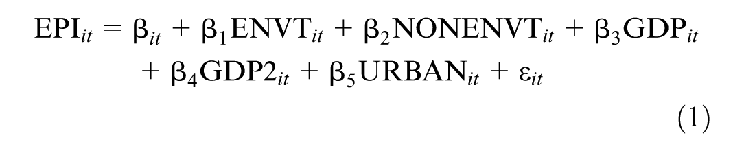
\begin{matrix} EP I_{i t} = β_{i t} + β_{1} ENV T_{i t} + β_{2} NONENV T_{i t} + β_{3} GD P_{i t} \\ + β_{4} GDP 2_{i t} + β_{5} URBA N_{i t} + ε_{i t} \end{matrix}

(1)

In the model, the index “i” represents cross-sections (different countries) with 1, 2, 3, …, N, and the index “t” represents time periods (years) with 1, 2, 3, …, T. In addition, the error term “è” represents the differences between the model’s predictions and the actual observations. Based on this structure, the order of the analysis method used is presented in detail below.

Cross-Sectional Dependence Test

In panel data analyses, it is generally assumed that the units are independent from each other. However, as economic, political and social ties between countries have strengthened with globalization, the validity of this assumption is questionable. In particular, the possibility that economic or political shocks in one country may spread to other countries makes the issue of cross-sectional dependence (CSD) important. Therefore, in order for the model results to be reliable, the correlation between units should be tested and appropriate analysis methods should be used. In this study, Pesaran (2004) CDLM test and Pesaran et al. (2008) CDLM_adj test are applied to test for cross-sectional dependence in the panel data set of OECD countries.

Unit Root Test

If cross-sectional dependence is detected among the series, second generation unit root tests are used. In this study, the CIPS test developed by Pesaran (2007) is used for stationarity analysis. This test provides an analysis suitable for panel data structure by considering lagged values and differences of each unit to determine whether the series are stationary or not. The CIPS test results are interpreted by comparing them with the critical table values. If the test statistic is less than the absolute value of the critical value, the series is considered to contain a unit root, while if it is greater than the critical value, the series is stationary.

Homogeneity Test

When checking for effects in panel data models, it is crucial to test whether the slope coefficients are equal across all units. To this end, we employ the Slope Homogeneity Test of Pesaran and Yamagata (2008). This tests further if there is a significant difference between slope coefficients across the countries present in the panel.

Cointegration Test

The cointegration analysis utilizes the Durbin–Hausman cointegration test of Westerlund (2008), as the model exhibits both cross-sectional dependence and coefficient heterogeneity. The test provides the opportunity to examine series under the assumption that some of the independent variables of the series are stationary (I[0]), while others are at first order (I[1]). The two different statistics were DHg the group mean statistic calculated under the heterogeneity assumption and DHp the panel statistic calculated under the homogeneity assumption.

Coefficient Estimation

In this study, quantile regression analysis is adopted as the basic coefficient estimation method. An important development in the application of quantile regression in panel data analysis is The Panel Quantile Regression for Panel Data (QRPD) method, introduced by Powell (2022), incorporating non-additive fixed effects. The QRPD method can provide consistent estimates even in cases where the time dimension (T) is limited and provides the opportunity to effectively model country-specific fixed effects. Unlike traditional panel quantile regression techniques, this method offers an analytical advantage by separating error terms and focusing on the time-dependent dynamics of the variables. The QRPD method stands out as an effective tool especially in cases where heterogeneous structures and different distribution characteristics need to be examined in detail. This method allows for understanding how the relationships between variables vary across different quantile levels, while also offering more reliable and robust results by accounting for the dynamics of the panel data structure. This flexible structure of QRPD allows for a more accurate analysis of each component of the model and reinforces the validity of the model by best reflecting heterogeneous structures. Therefore, we selected QRPD over alternative panel quantile regression methods, as it provides the most consistent and appropriate framework for addressing the heterogeneity and distributional differences in our OECD dataset.

Empirical Analysis Results

As discussed in detail in the methodology section, the first stage of the analysis process examined the existence of CSD in the variables and the model. This stage is of critical importance in determining possible dependency relationships between cross-sectional units in panel data analysis. The findings are summarized in Table 2, which explains the effects of cross-sectional dependency on the model in more detail.

Table 2.

Results of Cross-Sectional Dependence (CSD) Tests for OECD Panel Data.

Test Statistic	EPI	ENVTO	NONENVTO	GDP	GDP2	URBAN	Model
CD_LM	93.608^a (.000)	130.093^a (.000)	131.438^a (.000)	124.763^a (.000)	124.692^a (.000)	68.171^a (.000)	37.508^a (.000)
CD_{LM adj}	279.893^a (.000)	432.870^a (.000)	442.111^a (.000)	411.005^a (.000)	410.698^a (.000)	419.92^a (.000)	411.737^a (.000)

There is cross-sectional dependence at the 1% significance level.

The CDLM and CDLM adj test results in the table reveal the existence of CSD at the 1% significance level for all variables. According to this finding, the detection of the existence of CSD for variables affecting environmental quality may indicate the existence of common economic and environmental shocks among countries. Therefore, methods that take CSD into account should be used in panel data analysis, and traditional estimation methods may give misleading results.

As CSD was identified in the series, the detailed results of the CIPS test, which is part of the second-generation unit root tests, can be found in Table 3.

Table 3.

Results of Unit Root Tests for Panel Variables.

Variables	CIPS statistics
Variables	Level	1. Difference
EPI	−1.894	−3.069^a
ENVT	−2.753^b	—
NONENVT	−2.997^a	—
GDP	−2.487	−3.445^a
GDP2	−2.450	−3.441^a
URBAN	−2.760^b	—

Note. For the table, the critical values at the 1% and 5% significance levels are −2.79 and −2.65. The letters a and b denotes significance at the 1% and 5% levels, respectively.

According to the unit root test results in Table 3, the EPI variable has a unit root at the level and becomes stationary at the 1% significance level in the 1st difference and exhibits the I(1) property. While the ENVT and NONENVT variables are stationary at the level and have the I(0) property, The GDP and GDP2 variables both exhibit a unit root at the level but are stationary at the 1% significance level in the 1st difference and exhibit the I(1) property; At the 5% significance level, the URBAN variable is stationary at the level values.

The third stage in the empirical analysis involves the application of the Delta test proposed by Pesaran and Yamagata (2008) to evaluate the heterogeneity properties of the model. The test is essential for confirming the reliability of the cointegration and coefficient estimation analyses. The findings of the test are presented in detail in Table 4 below.

Table 4.

Results of Slope Homogeneity Tests for Panel Data.

Test Statistic	Statistics	Prob.
Delta_tilde	30.198^a	.000
Delta_tilde_adj	35.087^a	.000

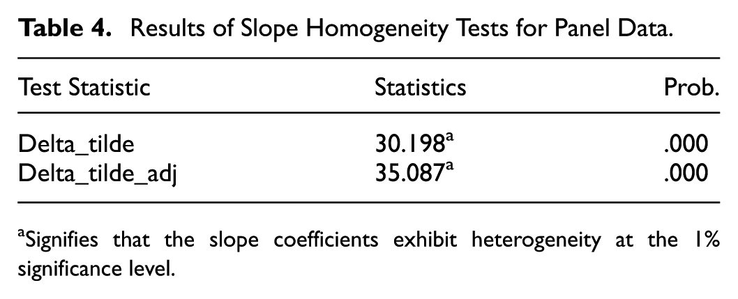
Signifies that the slope coefficients exhibit heterogeneity at the 1% significance level.

The homogeneity test results presented in Table 4 show that Delta_tilde statistics are 30.198 and Delta_tilde_adj statistics are 35.087, and the p-value of both tests is .000. These results show that the slope coefficients are heterogeneous at 1% significance level. This situation reveals that the independent variables used to explain environmental quality (EPI) environmental goods trade (ENVT), non-environmental goods trade (NONENVT), economic growth (GDP), squared expression of economic growth (GDP2) and urbanization (URBAN)) have different effects for each observation unit. These findings show that factors such as environmental goods trade, non-environmental goods trade, economic growth, squared effect of growth, and urbanization can have different levels of effect on environmental quality.

In the fourth stage of the analysis, cointegration test was applied to determine the long-term relationships between the series. In this context, considering the determination of CSD in the model and the fact that some of the variables have integration at I(0) and some at I(1) level, as well as the heterogeneity of the slope coefficients, the Durbin–Hausman test was preferred. Table 5 below presents the results of this test.

Table 5.

Results of Cointegration Tests for OECD Panel Data.

Tests	Statistics	Prob.
DHg	13.734^a	.000
DHp	22.595^a	.000

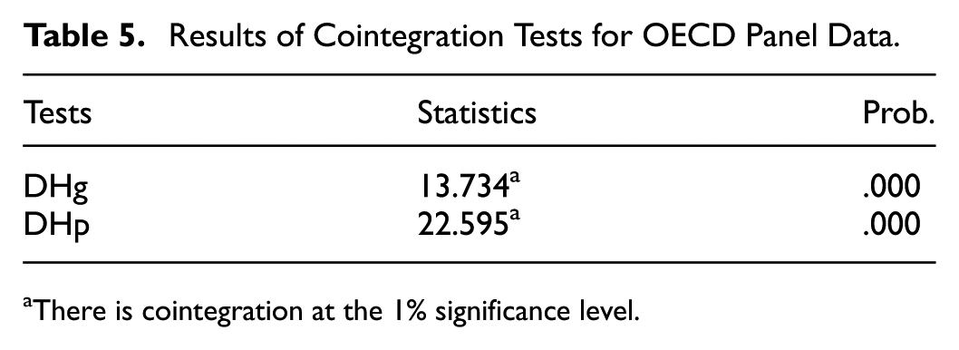
There is cointegration at the 1% significance level.

The cointegration test results in Table 5 show that the DHg statistic is 13.734 and the DHp statistic is 22.595, and the p-value of both tests is .000. The findings demonstrate a cointegration relationship between the series at the 1% significance level, suggesting a significant long-term relationship between environmental quality (EPI) and the explanatory variables. The cointegration test reveals that these variables are in a mutually balanced relationship in the long term. This reveals that the steps to be taken to improve environmental quality should be in harmony not only with current economic and trade policies, but also with long-term structural changes. In this context, the effects of factors such as economic growth, trade and urbanization on environmental quality can also be shaped by long-term policies. When creating policies and implementing strategies aimed at improving environmental quality, it is of great importance to consider the effects of economic growth and trade on the environment. In this direction, it can be said that policies should be developed to increase environmental quality in a sustainable way.

During the fifth stage of the analysis, the QRPD method was applied, which facilitates long-term estimations by accounting for the heterogeneous structure of both CSD and slope coefficients, as indicated by the pre-test results. This method was preferred because it reveals the effects of the variables in the model over time in a more precise and consistent manner. Table 6 presents a detailed overview of the coefficient estimation results.

Table 6.

QRPD Coefficient Estimates Across Quantiles for OECD Countries.

Dependent variable: EPI
Variables	Quantiles					OLS
Variables	.10	.25	.50	.75	.90	OLS
ENVT	.183^a (.000)	.047^a (.000)	.114^a (.000)	.084^a (.000)	.053^a (.000)	.092^a (.000)
NONENVT	−.103^a (.000)	−.052^a (.000)	−.106^a (.000)	−.049^a (.000)	−.029^a (.000)	−.021 (.157)
GDP	−.045^a (.000)	−.058^a (.000)	.024 (.724)	−.261^a (.000)	−.769^a (.000)	−.199^a (.003)
GDP2	.002^a (.000)	.002^a (.000)	.002^c (.071)	.006^a (.000)	.016^a (.000)	.005^a (.000)
URBAN	−.187^a (.000)	−.146^a (.000)	−.157^a (.000)	−.101^b (.000)	−.135^a (.000)	−.148^a (.000)

Note. a, b, and c indicate that the coefficients are statistically significant at the 1%, 5% and 10% significance levels, respectively.

Upon examining the QRPD results in Table 6, it is first noteworthy that the largest coefficient magnitudes are observed for GDP and URBAN, both exerting substantial negative effects on environmental quality, particularly at higher quantiles. Compared to these variables, the coefficients of trade-related variables are smaller in size but still meaningful in indicating the role of trade composition. Specifically, the effect of EVNT, one of the key independent variables representing trade in environmental products, on environmental quality is positive across all quantiles. In other words, an increase in trade of environmental products leads to an improvement in environmental quality. However, the strength of the effect decreases at high quantiles. For example, while the effect strength is .183 at quantile .10, it decreases to .084 and .053 at quantiles .75 and .90. Interpreting coefficients as elasticities, a 10% increase in environmental-goods trade is associated with an ≈.18%, .08%, and .05% increase in the EPI at the .10, .75, and .90 quantiles, respectively. This suggests that the impact of trade in environmental goods is decreasing in countries with higher environmental quality. These distributional patterns suggest that gains from environmental-goods trade are larger for OECD countries with lower baseline environmental performance, whereas high-performing countries experience smaller marginal improvements, consistent with heterogeneity stemming from differences in industrial structure, energy mix and policy history. The effect of trade in non-environmental goods (NONENVT), another key independent variable, on environmental quality is negative in most of the quantiles. Accordingly, an increase in trade in non-environmental products has a decreasing effect on environmental quality. As the quantile level increases, the strength of the effect weakens. In other words, the deteriorating effect of trade in non-environmental products on environmental quality is more pronounced in low quantiles and its effect decreases as environmental quality increases.

The diminishing marginal impact of environmental goods trade at higher quantiles of environmental quality can be attributed to a saturation effect. In high-performing OECD countries, environmental standards are already stringent, and clean technologies are widely adopted, leaving less room for trade-driven improvements. Furthermore, these countries are experiencing technological convergence, where the incremental benefits of importing or exporting additional environmental goods are smaller compared to developing countries. This suggests that, while trade in environmental goods remains significant, further gains in high-performing economies are likely to be achieved through policy innovation, circular economy practices, and sustainable consumption strategies, rather than trade flows alone.

When the econometric findings of the study are evaluated within the theoretical framework of the effects of environmental and non-environmental products on environmental quality, the following conclusions are reached. The findings of the study show that trade in non-environmental goods reduces environmental quality due to the scale effect, but trade in environmental goods can offset this negative scale effect. In particular, trade in renewable energy equipment, air-water pollution control systems and energy efficient technologies can mitigate the negative environmental consequences of the scale effect. It shows that trade in environmental goods can improve environmental quality through the composition effect, while trade in non-environmental goods can negatively affect the environment by steering some countries towards carbon-intensive sectors. Therefore, trade policies should be implemented to encourage the development of environmentally friendly sectors, while sustainable production should be promoted for countries that depend on non-environmentally friendly sectors. It shows that trade in environmental goods improves environmental quality through technical effects, but trade in non-environmental goods fails to stimulate technical development. Especially in developing countries, imports of cleaner production technologies should be increased, and industrial policies should be supported in this direction. Their finding that trade in environmental goods improves environmental quality may provide indirect evidence that the Regulatory Spillover Effect is at work in OECD countries. Trade in environmental goods can promote regulatory harmonization by converging countries’ renewable energy policies, waste management systems and air-water pollution regulations. Especially in countries with weak environmental regulations, imports of environmental goods can trigger the strengthening of environmental policies. The fact that trade in environmental products improves environmental quality may indicate that the Rationalization Effect operates in environmental product sectors. However, the fact that trade in non-environmental goods reduces environmental quality may indicate that this effect does not work to the same degree in all sectors or that in some sectors the effect of trade to favor efficient firms does not provide environmental benefits. Especially in areas such as renewable energy, waste management and water treatment technologies, it can be concluded that trade improves environmental quality by enabling greener firms to gain a competitive advantage.

The economic growth (GDP) variable, used to test the validity of the EKC hypothesis, has a generally negative impact on environmental quality. This suggests that as economic growth rises, environmental quality declines. When the quantiles are taken into consideration, the deteriorating effect on environmental quality increases as the quantile level increases. For example, while the negative effect is .045 in the .10th quantile, it is .769 in the .90th quantile. The GDP2 variable, which is used to represent higher levels of economic development and includes the squared expression of economic growth, positively affects environmental quality. This result reveals that higher levels of economic development improve environmental quality. In terms of quantiles, it is observed that the positive effect, which is generally low, increases at higher quantiles. For example, while the effect strength was .002 at quantile .10, it was .006 and .016 at quantiles 9.75 and .90. These findings suggest that GDP2 improves environmental quality and that the improving effect becomes more pronounced as environmental quality increases. Moreover, the findings also support the validity of the EKC hypothesis. To provide greater clarity on the EKC hypothesis, we also calculated the turning points based on the standard formula C = −βGDP/(2 × βGDP2; Dinda, 2004; Hasanov et al., 2021; Stern, 2004). Since the variables are used in logarithmic form, the results are expressed in log-GDP units. The findings indicate that the turning point is reached at approximately 11.25 (τ = .10), 14.50 (τ = .25), 21.75 (τ = .75), 24.03 (τ = .90), and 19.90 in the OLS estimation. These results suggest that the income level at which environmental quality begins to improve varies considerably across quantiles: countries with lower environmental performance reach the turning point at relatively lower income levels, while in higher-performing countries the threshold shifts to substantially higher income levels. At the median quantile (τ = .50), however, the EKC pattern is not observed, and therefore no meaningful turning point is reported.

Finally, the Urbanization (URBAN) variable is found to reduce environmental quality, with the decreasing effect being less pronounced at higher quantiles. For example, while the negative effect was .187 at quantile .10, it was .135 at quantile .90. This indicates that the negative impact of urbanization will decrease as environmental quality increases. These findings suggest that policies to improve environmental quality should focus on trade in environmental goods, but the negative effects of trade in non-environmental goods should be minimized. Moreover, it is important to develop sustainable growth and urbanization strategies to reduce the negative effects of economic growth and urbanization on environmental quality.

OLS results are also presented in Table 6. Accordingly, OLS provides a single coefficient estimate for each independent variable and thus presents an average effect. The OLS results are generally similar to the QRPD results. Accordingly, trade in environmental goods has an increasing effect on environmental quality, while trade in non-environmental goods has a decreasing effect. The validity of the EKC hypothesis is also confirmed by these test results. As a result, the QRPD method offers a more detailed analysis compared to the OLS method, clearly illustrating how the impact of independent variables on the dependent variable varies across different quantile levels. This highlights the need for policies that consider the factors influencing environmental quality to be tailored according to the level of environmental quality.

Conclusion

This study investigates the impact of trade in environmental and non-environmental goods on environmental quality in OECD countries. For this purpose, quantile regression and panel data analysis are used. The findings show that trade in environmental goods has a positive impact on environmental quality, especially in countries with low to medium environmental standards. Conversely, trade in non-environmental goods is found to have a detrimental effect on environmental quality in all cases.

The study also analyzed the impact of economic growth on environmental quality and confirmed the validity of the Environmental Kuznets Curve (EKC) hypothesis in line with the empirical findings. Accordingly, although economic growth negatively affects environmental quality in the first stage, this effect is reversed at a certain level of prosperity thanks to environmental protection policies and long-term technological development (Feng et al., 2022). On the other hand, the coefficient for the urbanization variable is found to be negative, indicating that urbanization has a negative effect on environmental quality in all quantiles and this effect is stronger in countries with low environmental quality.

The study examines at the combination of trade in environmental and non-environmental goods and the impact of such on environmental quality in OECD countries, concluding that trade in environmental goods (i.e., sustainability technologies) improves environmental quality across all OECD countries but particularly so in low and medium environmental standards countries, and that trade in non-environmental goods largely causes environmental degradation. These findings are in line with Zugravu-Soilita (2019), who emphasizes that while trade in environmental goods increases productivity by reducing emissions per unit of GDP, its overall environmental impact varies depending on the country’s trade profile. Similarly, Zhang et al. (2023) argues that carbon emissions trading policies and firm-level environmental strategies play an important role in shaping the sustainability benefits of export product quality. Additionally, Zugravu-Soilita (2018) argued that trade in environmental goods is likely to reduce air pollution from the technology spillover it causes but is likely to increase water pollution from scale and composition effects. Hence, there is a need for targeted environmental policy to measure different pollutants and industries. Wan (2018) further established that, on its own, trade liberalization of environmental goods does not necessarily lead to environmental improvement and emphasized the need for accompanying regulatory system. Policymakers must focus on interventions that encourage diffusion of cleaner technologies, while also strengthening enforcement of environmental regulations, to control possible adverse impacts of trade in goods that relate to the environment.

As per the findings, policy makers should put in place measures that promote trade in environmental goods, in order to help improve environmental quality as well as strategies to mitigate the harmful effect from trade of non-environmental goods. Moreover, policies for sustainable growth also need to take into account, environmental repercussions of economic growth in the long term, as well as the usage of eco-friendly technologies. To lessen the environmental impact connected to urban processes, the last suggestion is to advocate for sustainable urban planning policies. In addition, policy priorities can be tailored to the different environmental quality levels of OECD countries. In countries that are still struggling with lower environmental performance, the focus should be on improving energy efficiency, restructuring industries with high pollution intensity, and making greater use of cleaner technologies, especially in energy and manufacturing. Countries at an intermediate level of performance may benefit most from accelerating investments in renewable energy, improving waste management, and strengthening the protection of water resources. For the high-performing OECD members, where the marginal benefits of further trade in environmental goods are limited, the next step is more likely to come from policy innovation, the adoption of circular economy models, and encouraging sustainable consumption habits, particularly in transport, agriculture, and consumer markets. Differentiating policy directions in this way can help OECD countries design strategies that are better aligned with their specific environmental challenges.

This study has several limitations. First, as the EPI is a composite index, it does not reveal sector-specific effects of trade on different environmental dimensions (e.g., air, water, biodiversity). Future research could conduct disaggregated analyses using EPI sub-components. Second, potential reverse causality remains a concern: countries with higher environmental quality may be more engaged in environmental goods trade. Although the applied econometric framework (cointegration, QRPD) mitigates this issue, it cannot be fully eliminated. Instrumental variables, GMM estimators, or natural experiments could provide stronger identification. Third, differences in environmental governance and policy rigidity are not directly controlled for; including indicators such as the OECD Environmental Policy Rigidity Index would enhance future studies. Fourth, emissions from trade-related transport are excluded, which may understate total impacts. Integrating MRIO database would enable separation of production- and transport-related emissions. Moreover, while the study shows an inverse link between urbanization and environmental quality, this relationship may not be strictly linear; future research should test for possible thresholds or non-linear dynamics. Finally, the focus on OECD countries limits generalizability, as non-OECD contexts often differ in traded-goods composition (e.g., greater reliance on resource-intensive or low-tech exports) and institutional capacity (e.g., weaker regulatory enforcement). Future research should extend the analysis to developing and emerging economies to assess whether the mechanisms identified here persist under different industrial structures and governance regimes.

Footnotes

ORCID iD

Ali Altıner

Ethical Considerations

This study did not involve human participants or animals. The analysis relied exclusively on publicly available secondary data; therefore, ethical approval and informed consent were not required. The research complies with internationally accepted standards for research practice and reporting.

Consent to Participate

Not applicable.

Consent for Publication

All authors consent to publish in the journal of “Sage Open.”

Funding

The authors disclosed receipt of the following financial support for the research, authorship, and/or publication of this article: This study has been supported by the Recep Tayyip Erdoğan University Development Foundation (Grant number: 02025004030452).

Declaration of Conflicting Interests

The authors declared no potential conflicts of interest with respect to the research, authorship, and/or publication of this article.

Data Availability Statement

The data used in this study are publicly available from the World Bank Open Data platform and the International Monetary Fund (IMF) databases. These sources provide unrestricted access to the data used for analysis in this article.

References

Alvi

Ahmad

Rehman

(2023). Trade of environmental versus non-environmental goods and carbon emissions in high and middle-income countries. Environmental Science and Pollution Research, 30, 65283–65295. https://doi.org/10.1007/s11356-023-26972-9

Antweiler

Copeland

B. R.

Taylor

M. S.

(2001). Is free trade good for the environment? American Economic Review, 91(4), 877–908. https://doi.org/10.1257/aer.91.4.877

Awan

Kocoglu

Subhan

Utepkaliyeva

Hossain

M. E.

(2025). Assessing energy efficiency in the built environment: A quantile regression analysis of CO2 emissions from buildings and manufacturing sector. Energy and Buildings, 338, Article 115733.

Bernauer

Nguyen

(2015). Free trade and environmental protection. Global Environmental Politics, 15(1), 1–20. https://doi.org/10.1162/GLEP_a_00279

Block

Emerson

J. W.

Esty

D. C.

de Sherbinin

Wendling

Z. A.

(2024). 2024 Environmental Performance Index. Yale Center for Environmental Law & Policy.

Can

Ahmed

Mercan

Kalugina

O. A.

(2021). The role of trading environment-friendly goods in environmental sustainability: Does green openness matter for OECD countries? Journal of Environmental Management, 295, Article 113038.

Cantore

Cheng

C. F. C.

(2018). International trade of environmental goods in gravity models. Journal of Environmental Management, 223, 1047–1060. https://doi.org/10.1016/j.jenvman.2018.05.036

Cherniwchan

Copeland

B. R.

Taylor

M. S.

(2017). Trade and the environment: New methods, measurements, and results. Annual Review of Economics, 9(1), 59–85.

Copeland

B. R.

Taylor

M. S.

(1994). North–South trade and the environment. The Quarterly Journal of Economics, 109(3), 755–787.

10.

CIESIN. (2024). Center for International Earth Science Information Network. Retrieved September 10, 2024, from https://www.ciesin.columbia.edu/datasets/dataset-home.html

11.

De Alwis

J. M. D. D. J

. (2014). Environmental consequence of trade openness for environmental goods. Sri Lankan Journal of Agricultural Economics, 16, 79–98.

12.

Dinda

(2004). Environmental Kuznets curve hypothesis: A survey. Ecological Economics, 49(4), 431–455.

13.

Elmonshid

L. B. E.

Sayed

O. A.

Awad Yousif

G. M.

Eldaw

K. E. H. I.

Hussein

M. A.

(2024). The impact of financial efficiency and renewable energy consumption on CO2 emission reduction in GCC economies: A panel data quantile regression approach. Sustainability, 16(14), Article 6242.

14.

Esen

Ö.

Yıldırım

D. Ç.

Yıldırım

(2024). A quantile regression approach to assess the impact of water-related environmental innovations on water stress. Technological Forecasting & Social Change, 203, 123343. https://doi.org/10.1016/j.techfore.2024.123343

15.

Essandoh

O. K.

Islam

Kakinaka

(2020). Linking international trade and foreign direct investment to CO2 emissions: Any differences between developed and developing countries? Science of the Total Environment, 712, Article 136437.

16.

Feng

Chen

(2022). Impact of environmental information disclosure policy and trade on Chinese paper industry environmental effects. International Journal of Environmental Research and Public Health, 19(18), Article 11614. https://doi.org/10.3390/ijerph191811614

17.

Grether

J.-M.

Mathys

N. A.

de Melo

(2009). Scale, technique and composition effects in the manufacturing industry. Journal of Environmental Economics and Management, 58(1), 46–63. https://doi.org/10.1016/j.jeem.2008.08.001

18.

Grossman

G. M.

Krueger

A. B.

(1991). Environmental Impacts of a North American Free Trade Agreement. National Bureau of Economic Research.

19.

Hasanov

F. J.

Hunt

L. C.

Mikayilov

J. I.

(2021). Estimating different order polynomial logarithmic environmental Kuznets curves. Environmental Science and Pollution Research, 28(31), 41965–41987.

20.

Pollitt

Pirie

Mercure

J.-F.

Liu

Meng

Tao

(2020). The impacts of the trade liberalization of environmental goods on power system and CO2 emissions. Energy Policy, 140, Article 111173. https://doi.org/10.1016/j.enpol.2019.111173

21.

Işık

Bulut

Ongan

Islam

Irfan

(2024). Exploring how economic growth, renewable energy, internet usage, and mineral rents influence CO2 emissions: A panel quantile regression analysis for 27 OECD countries. Resources Policy, 92, Article 105025.

22.

International Monetary Fund (IMF). (2021). Trade in environmental goods. https://climatedata.imf.org/documents/ad5179b954ed4a8389bf6400324a901e/explore

23.

International Monetary Fund (IMF). (2025a). Climate Change Indicators Dashboard. https://climatedata.imf.org/datasets/8636ce866c8a404b8d9baeaffa2c6cb3_0/about

24.

International Monetary Fund (IMF). (2025b). Direction of Trade Statistics (DOTS). https://data.imf.org/?sk=9d6028d4-f14a-464c-a2f2-59b2cd424b85

25.

Kreickemeier

Richter

P. M.

(2013). Trade and the environment: The role of firm heterogeneity. Review of International Economics, 22(2), 209–225. https://doi.org/10.1111/roie.12092

26.

Krugman

P. R.

Obstfeld

Melitz

M. J.

(2017). International economics: Theory and policy, the latest edition. Addison-Wesley.

27.

Levinson

(2009). Technology, international trade, and pollution from US manufacturing. American Economic Review, 99(5), 2177–2192.

28.

Liu

Zhang

Lei

(2022). Do imported environmental goods reduce pollution intensity? The end use matters. Energy Economics, 112, Article 106130. https://doi.org/10.1016/j.eneco.2022.106130

29.

Mao

Liu

Gui

Wang

(2023). Toward inclusive list-making for trade liberalization in environmental goods to reduce carbon emissions. Geography and Sustainability, 4, 200–212. https://doi.org/10.1016/j.geosus.2023.04.002

30.

Muhammad

Long

Salman

Dauda

(2020). Effect of urbanization and international trade on CO2 emissions across 65 belt and road initiative countries. Energy, 196, Article 117102.

31.

Muradian

O’Connor

Martines-Alier

(2002). Embodied pollution in trade: Estimating the ‘environmental load displacement’ of industrialised countries. Ecological Economics, 41(1), 51–67.

32.

Pesaran

M. H.

(2004). General diagnostic tests for cross section dependence in panels. Cambridge Working Papers in Economics, 1240(1), Article 1.

33.

Pesaran

M. H.

(2007). A simple panel unit root test in the presence of cross-section dependence. Journal of Applied Econometrics, 22(2), 265–312.

34.

Pesaran

M. H.

Ullah

Yamagata

(2008). A bias-adjusted LM test of error cross-section independence. The Econometrics Journal, 11(1), 105–127.

35.

Pesaran

M. H.

Yamagata

(2008). Testing slope homogeneity in large panels. Journal of Econometrics, 142(1), 50–93.

36.

Powell

(2022). Quantile regression with nonadditive fixed effects. Empirical Economics, 63(5), 2675–2691.

37.

Rom

Guillotreau

(2024). Mismanaged plastic waste and the environmental Kuznets curve: A quantile regression analysis. Marine Pollution Bulletin, 202, Article 116320.

38.

Sadorsky

(2012). Energy consumption, output and trade in South America. Energy Economics, 34(2), 476–488.

39.

Sauvage

(2014). The stringency of environmental regulations and trade in environmental goods (OECD Trade and Environment Working Papers, 2014/03). OECD Publishing.

40.

Shahbaz

Nasir

Roubaud

(2018). Environmental degradation in France: The effects of FDI, financial development, and economic growth. Energy Economics, 74, 843–857. https://doi.org/10.1016/j.eneco.2018.07.020

41.

Shen

Cui

Wei

Y. D.

Wang

(2024). Domesticating sustainability transitions: Spatial and temporal variation of industrial eco-efficiency in China. Applied Geography, 173, Article 103452. https://doi.org/10.1016/j.apgeog.2024.103452

42.

Steenblik

(2005). Environmental goods: A comparison of the APEC and OECD lists. https://www.oecd.org/environment/envtrade/35837840.pdf

43.

Stern

D. I.

(2004). The rise and fall of the environmental Kuznets curve. World Development, 32(8), 1419–1439.

44.

Ul-Durar

Arshed

De Sisto

Nazarian

Sadaf

(2024). Modeling green energy and innovation for ecological risk management using second generation dynamic quantile panel data model. Journal of Environmental Management, 366, Article 121741.

45.

UNEP. (2013). Green economy and trade: Trends, challenges and opportunities. https://www.unep.org/resources/report/green-economy-and-trade-trends-challenges-and-opportunities

46.

Wan

(2018). Trade liberalization and environmental goods: The role of environmental policy in shaping trade impacts. Ecological Economics, 146, 321–330. https://doi.org/10.1016/j.ecolecon.2017.10.009

47.

Wang

(2024). Rethinking the environmental Kuznets curve hypothesis across 214 countries: the impacts of 12 economic, institutional, technological, resource, and social factors. Humanities and Social Sciences Communications, 11(1), 1–19.

48.

Wei

Jiandong

Saleem

(2023). The impact of renewable energy transition, green growth, green trade, and green innovation on environmental quality: Evidence from top 10 green future countries. Frontiers in Environmental Science, 10, Article 1076859. https://doi.org/10.3389/fenvs.2022.1076859

49.

Westerlund

(2008). Panel cointegration tests of the fisher effect. Journal of Applied Econometrics, 23, 193–233. https://doi.org/101002/jae.967

50.

Wolf

M. J.

Emerson

J. W.

Esty

D. C.

de Sherbinin

Wendling

Z. A.

(2022). 2022Environmental Performance Index. Yale Center for Environmental Law & Policy.

51.

World Bank. (2025). World Development Indicators. Retrieved September 25, 2024, from https://databank.worldbank.org/reports.aspx?source=world-development-indicators

52.

World Trade Organization. (2014, July 8). Environmental Goods Agreement (EGA): Plurilateral negotiations among a group of WTO members. https://www.wto.org/english/tratop_e/envir_e/ega_e.htm

53.

YCELP. (2024). Environmental Performance Index. Retrieved November 10, 2024, from https://epi.yale.edu/

54.

Zhang

Kong

Wang

Vigne

S. A.

(2023). Exquisite workman through net-zero emissions? The effects of carbon emission trading on firms' export product quality. Energy Economics, 123, 106701. https://doi.org/10.1016/j.eneco.2023.106701

55.

Zugravu-Soilita

(2018). The impact of trade in environmental goods on pollution: Evidence from Central and Eastern European transition economies. Economic Modelling, 72, 159–174. https://doi.org/10.1016/j.econmod.2018.01.001

56.

Zugravu-Soilita

(2019). Trade in environmental goods and air pollution: A mediation analysis to estimate total, direct and indirect effects. Environmental and Resource Economics, 74, 1125–1162. https://doi.org/10.1007/s10640-019-00363-6

Assessing the EKC Hypothesis and the Impact of Environmental and Non-Environmental Goods Trade on Environmental Quality: Evidence from QRPD for OECD Countries

Abstract

Plain Language Summary

Keywords

Introduction

Theoretical Framework

Literature Review

Variables, Data, and Methodology

Variables

Data

Methodology

Cross-Sectional Dependence Test

Unit Root Test

Homogeneity Test

Cointegration Test

Coefficient Estimation

Empirical Analysis Results

Conclusion

Footnotes

ORCID iD

Ethical Considerations

Consent to Participate

Consent for Publication

Funding

Declaration of Conflicting Interests

Data Availability Statement

References