
Abstract
Considering the farmer’s decision of quitting cotton plantation due to low economic incentives, the current research is intended to evaluate the economic viability of cotton growers in Punjab. A comprehensively pretested questionnaire was used to gather the information from 240 cotton growers in face-to-face interviews. The cost–benefit ratio was estimated by calculating incurred variable costs, revenue generated, net farm income, and gross margin. The data envelopment analysis was applied to explore the economic, technical, and allocative efficiencies of the cotton producers. The second-stage regression analysis was also conducted to evaluate the socioeconomic factors affecting farmer’s efficiencies by applying the Tobit regression model. The small farmers were found to be most vulnerable group with low returns on investments and low technical and economics efficiencies score. The results also indicate that the financial constraints, difficulty to access agriculture credit, access to extension services, and lack of formal education are the main factors affecting farmer’s efficiency. The government should regulate the input prices and agriculture department should provide formal training to the farmers to adopt better management practices to reduce cost of production.
Keywords
Introduction
Cotton production is an integral part of the national economy. Pakistan is the fifth largest cotton producer and the third largest exporter of the raw cotton in the world (International Cotton Advisory Committee, 2019). Cotton acquires a special status of industrial cash crop in Pakistan. It is the major source of input to textile sector, that is, the largest industrial sector of the country employing 40% of the country’s total labor force (Government of Pakistan [GOP], 2019). Cotton and allied textile products are not only the key component of foreign exchange earnings but also a prominent source of livelihood, about 1.6 million farmers are growing cotton on the 15% of the nation’s land (U.S. Department of Agriculture [USDA], 2019).
Considering cotton’s pervasive forward and backward linkages, it resides a significantly important position in the progress of rural sector of the country. The performance of cotton is major factor of development not only for agriculture sector but also has a significant impact on the economic development of the country. Cotton contributed about 4.5% to agricultural value addition during the production year 2018–2019 (GOP, 2019). Cotton is considered as a promising source of fiber all around the world and cotton seed provides edible oil to meet 64% of the nation’s edible oil demand (Abid et al., 2011). Whereas, byproduct of cotton seed that is known as seed cake is also an essential and healthy component of animals feed.
However, during the production period of 2018–2019, cotton played a significant role by contributing 8% to gross domestic product and 11.11 billion dollars earnings from the export of cotton and allied products (State Bank of Pakistan, 2019). But in fact, the production of cotton was decreased by 17% from 11.946 million bales to 9.861 million bales as compared to previous production period. The area under cotton plantation was also decreased from 2,700,000 to 2,373,000 hectares (GOP, 2019). In addition to that, Pakistan cotton yield per hector in 2018–2019 was ranked as 10th in the world because the average cotton production per hectare was low compared with other competitive countries (Shahbaz et al., 2019). The most important reason behind low production and contraction of area for cotton production is low economic incentives to the farmers and others such as tough weather conditions, insect and pest, and disease attacks (GOP, 2019).
Among 1.6 million cotton growers in Pakistan, 81% are small farmers with landholdings less than 5.7 hectares (USDA, 2019). Unfortunately, large farmers in Pakistan have a significant influence in agriculture and have easy access to resources and modern technology (Kousar et al., 2006), whereas the small and medium farmers are facing common constraint, that is, resource availability, technical support, credit facility, and access to extension services. It is worth mentioning that farmer’s planting decisions are driven by expected prices in addition to factors such as relative cost of production from competing crops, input availability, and government support (USDA, 2019). The recent decrease in production and shift in farmer’s decisions to plant other crops instead of cotton makes this research significant to investigate the farmer’s economic incentive and factors affecting the grower’s efficiencies. This study also aims to draw a comparison among cotton farmers with different land holdings to carefully investigate the economic, allocative, and technical efficiencies.
The five aspects of the present research are the main contribution to the existing literature. First, keeping in view the farmers’ decisions of quitting cotton plantation due to low economic incentives, the study is intended to calculate the cost–benefit analysis of the cotton growers in the research zone. The second contribution of the present research is to evaluate the economic, allocative, and technical efficiencies with respect to farm size to carefully explore the most vulnerable group. The third impact of the present research is to investigate the major factors affecting the low average production of cotton by estimating the economic and technical and allocative inefficiencies. Fourth, to bridge the gap in the existing literature, it is indispensable to estimate economic efficiency (EE) using data envelopment analysis (DEA) and second-stage regression “Tobit regression model” to discover the impact of socioeconomic factors on inefficiencies of cotton farmers. The fifth contribution is to suggest the practical policy options to improve the economic and technical efficiency (TE) levels of the cotton growers to address the farmers’ decision of quitting cotton plantation due to low economic incentives.
The remaining of the article is arranged as follows: the second part of the study discusses the literature reviewed. The third part briefly explains data, variables, models, and methods for empirical analysis of this project. The fourth part discusses the results and validates their results with other studies. The fifth part consists of conclusion followed by the references at the end.
Literature Review
The cotton, being the promising source of livelihood and mainstay for national economy of Pakistan, had become the topic of keen interest for many international and local researchers such as Ashraf et al. (2018) who forecasted the area under cotton cultivation along with production and average yield of cotton in Punjab province of Pakistan by using the time series data from the year 1990–2017. The findings of the study revealed that area under cotton plantation and average yield of cotton decreased historically. Besides, the study also forecasted that the average yield of cotton will continue to decline in Punjab till 2025. There are other similar studies on cotton and cash crops in Pakistan, such as Ali et al. (2013, 2015), Shuli et al. (2018), and Tunio et al. (2016). Although all these studies provide a handful of information about the current and future situation of cotton by considering the time series data for different periods, but keeping in mind the contraction of area under cotton in Punjab Province, this study is unique to take primary data to evaluate the economic viability of cotton growers in Punjab province of Pakistan.
Plenty of studies had estimated the efficiency of different crops using parametric and nonparametric techniques: for example, Kizilaslan (2009) conducted a study using a nonparametric approach to investigate consumption efficiency for cherries production in Turkey; Mohammadi and Omid (2010) greenhouse cucumber in Iran; S. Singh et al. (1988) in six different agricultural climate zones in Indian Punjab; Ozkan et al. (2004) in greenhouse vegetables; Mandal et al. (2002) on soybean in India; Alimagham et al. (2017) on soybean in Iran; Pishgar-Komleh et al. (2012) on potato crop in Iran; Hatirli et al. (2005) in agriculture production in Turkey; G. Singh et al. (2004) on wheat production in India; Mohammadi et al. (2008) on potato in Iran; and Hatirli et al. (2006) on tomato in Turkey.
Data envelopment is a nonparametric analysis. DEA classifies decision-making units (DMUs) by benchmarking the best (DMU). One of the main advantages of DEA is that it can simultaneously evaluate several outputs and inputs (Zhang et al., 2009). In addition to that, DEA does not require any predefined assumptions to make a functional relationship among inputs and outputs, which makes DEA superior to other parametric models (Mousavi-Avval, Rafiee, Jafari, & Mohammadi, 2011). In recent times, DEA has vast applications in different research fields: Basso et al. (2018) measured the performance of the museum using DEA, and Lo Storto (2018) used DEA model to estimate the cycle efficiency of the airports in Italy. Application of DEA in agriculture also has significant importance: Mobtaker et al. (2012) applied DEA model to find energy optimization of alfalfa; Wang et al. (2018) carried out a study to maximize agriculture water use efficiency in China; Mousavi-Avval, Rafiee, and Mohammadi (2011) used DEA to estimate input cost and apple production in Iran; Khoshnevisan et al. (2013) applied DEA to reduce greenhouse gases (GHG) and energy efficiency in wheat production; Mardani and Salarpour (2015) estimated the efficiency of potato fields in Iran; Nassiri and Singh (2010) calculated the energy efficiency of paddy crop in India; and Abbas et al. (2018) studied the optimization of energy use on corn fields by applying DEA.
On the basis of the existing literature, there are few studies which applied DEA model to analyze EE in agriculture, that is, Song et al. (2018) applied DEA to probe economic growth and environmental efficiency of China. Ghiyasi (2017) applied DEA to examine cost and revenue efficiency. Ke-Fei (2015) designed EE of agriculture using DEA. Faisal et al. (2018) estimated economic and production efficiency of tobacco in Punjab, Pakistan. Imran et al. (2019) used DEA to compare the EE score of farmers who adopted climate-smart agriculture and non-adopters in central part of Punjab. Although plenty of the research has been carried out to estimate the efficiency of different crops in different parts of the world, literature is limited to estimate the economic compression of cotton growers on the basis of farm size especially in Punjab, Pakistan. Thus, to bridge the gap in the existing literature, this study applies DEA model to estimate economic, allocative, and technical efficiencies of the small, medium, and large cotton growers in the southern Punjab, Pakistan.
Research Methods
Project Zone
The Punjab province of Pakistan produces 80% of the total cotton produced in the country followed by Sindh Province (Zulfiqar et al., 2017). It is worth to mention that Punjab province has 37 districts, but cotton is primarily cultivated in 19 districts which are mostly located in southern part of Punjab province (for details see appendix) (Directorate of Agriculture [DOA], 2019). Thus, keeping in view the total share of cotton production and area under cotton cultivation, the 19 cotton-producing districts of Punjab were segregated for further random selection of two districts. The project zone is described in attached study map (Figure 1).
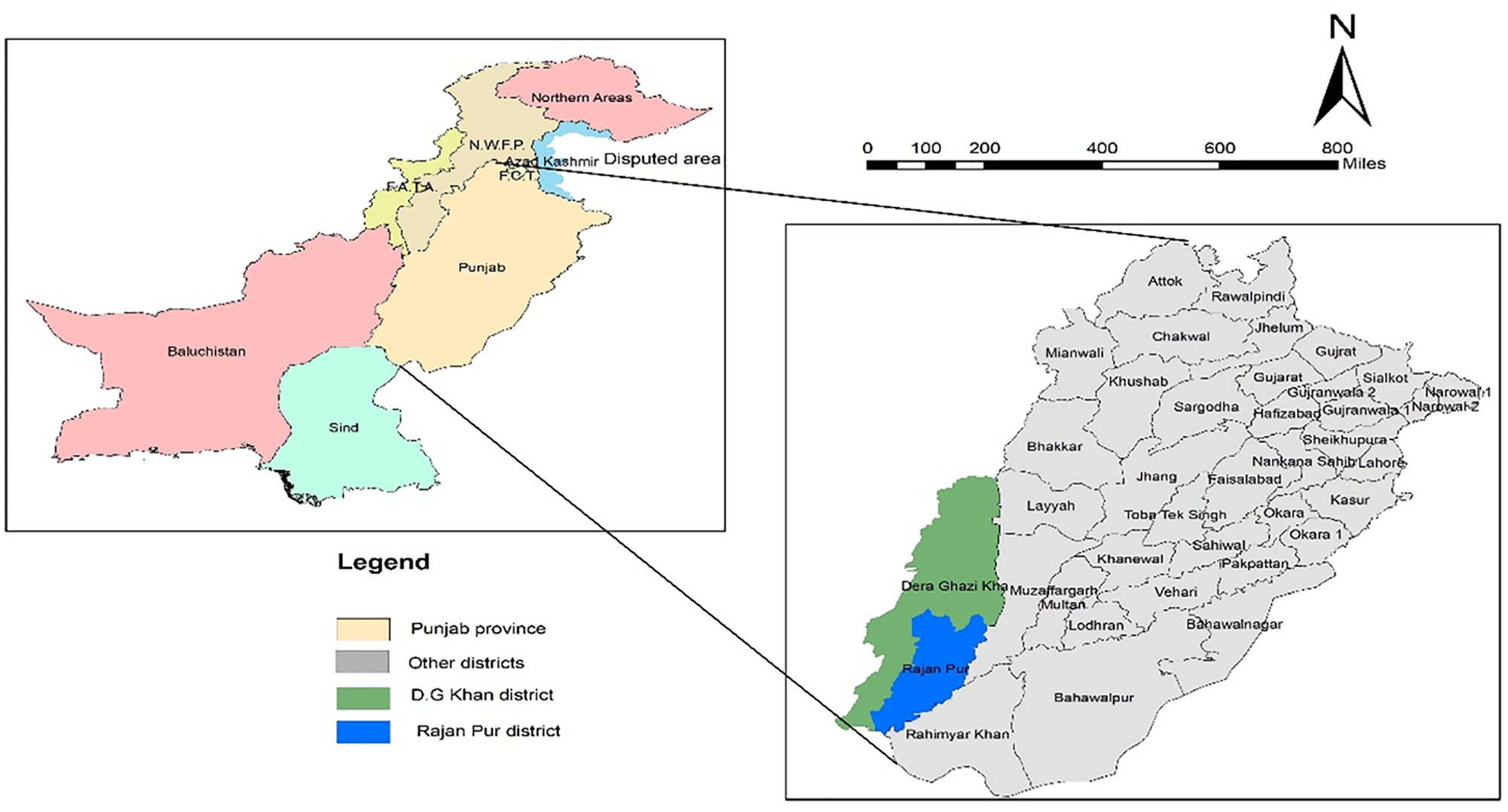
Project zone.
Sampling
The primary data was collected by applying a multistage random sampling technique from 19 cotton-producing districts of Punjab province. In the first step, districts D. G. Khan and Rajanpur were randomly selected from 19 cotton-producing districts. In the next stage, Tehsil Kot Chutta from district D. G. Khan, whereas tehsil Jampur from district Rajanpur were randomly selected. In the next step, three rural union council (UCs) were selected randomly from each selected tehsil. Later, in the next stage, two villages from each selected rural UC were randomly selected. In the last stage, 20 cotton growers were selected from each village by random sampling technique. Finally, input-output information was collected from 240 cotton farmers’ in-person interviews with 120 farmers from each district as given in Table 1.
Sample Selection by Multistage Random Sampling Technique.

Note. Author’s tabulations.
Prior to the study, a pretest survey was carried out to test the scope of the area, sample, and instrument. Furthermore, the farmers were categorized as large, medium, and small farmers with respect to the landholdings. The farmers with landholdings less than or equal to 6 and 12.5 acres were declared as small and medium farmers, respectively, whereas the farmers with land holdings greater than 12.5 acres were declared as large farmers.
Analytical Procedure
Different computer applications were used to perform empirical analysis, such as Microsoft Excel, SPSS, Stat-14.0, and DEAP-2.1. To evaluate the EE of cotton farmers, total costs and total revenue were calculated. The total variable cost covers seed price, land preparation, labor charges, fertilizers, chemicals, and irrigation charges. Whereas fixed cost was reflected by taking land rent as opportunity cost of the land (Akhtar et al., 2015). Net income, gross margin, and cost–benefit analysis were carried out according to given formulas (Faisal et al., 2018).

DEA
The efficiency of the firm means the comparison between maximum and current productivity (Farrel, 1957). The production frontier was applied to evaluate the maximum productivity of the farmers in this study. Two different methods (i.e., stochastic frontier analysis (SFA) and DEA) were adopted to develop the production frontier (Hiebert, 1974). The linear programming technique is applied in DEA technique. The difference between the estimated efficiency score and the actual score is the inefficiency score of the farmers (Faisal et al., 2018). DEA model estimates the efficiency of the firms using input- or output-oriented models. But, most of the studies related to agricultural subjects consider the input-oriented method, the reason being the growers can only control the inputs but not the outputs (Pahlavan et al., 2012). Therefore, this article also used input-oriented technique.
Furthermore, DEA input-oriented technique works on two basic assumptions: (a) contact return to scale and (2) variable return to scale (VRS). Coelli et al. (1998) suggested that DEA-CRS is more suitable when firms are operating at optimum level. But, due to many constraints, such as farm size, financial crisis, and credit facility, inputs availability makes it impossible for the farmers in Pakistan. Therefore, to mitigate these difficulties, Banker et al. (1984) presented DEA VRS method. Considering the objective and nature of the study, DEA VRS method is used to evaluate the efficiency of the cotton farmers in the study zone.
This study evaluated the farmers’ efficiency scores using input-oriented DEA with VRS property. The variables to evaluate the efficiency scores are as follows: the total output of each cotton grower was taken as output (Y) variable, whereas input variables include land preparation, seed rate, labor hours, fertilizers, chemicals, irrigation, and land rent.
TE
DEA-VRS input-oriented model was used to estimate the TE score of cotton growers as described by Mohammad (2009).

where Y shows the quantity of physical output for “N” cotton growers;
EE
The EE is defined as the minimum cost divided by actual cost, and it can be evaluated by applying DEA cost-revenue model (Faisal et al., 2018). The DEA cost minimization model can be expressed as in Equation 3.
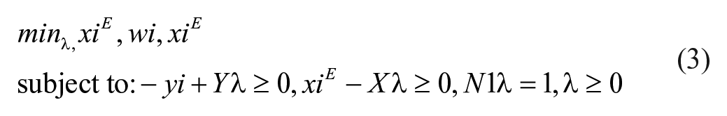
where
Economic efficiency = minimum cost/actual cost

Allocative efficiency
The allocative efficiency (AE) can be attained by dividing the EE by TE as given in Equation 5.

Tobit Model
The existing literature on efficiency estimation also investigates the factors causing inefficiencies and variations in farmer’s efficiency levels (Ibrahim & Omotesho, 2013). After estimating the economic, technical, and AE scores, the farmer’s inefficiency was estimated by subtracting the obtained efficiency scores from decimal one. The technical, economic, and allocative inefficiencies scores were taken as dependent variable. The DEA efficiency distribution lies from 0 to 1. It indicates that dependent variables are not normally distributed; therefore, to avoid biased estimation, this study applied Tobit regression model instead of ordinary least square as presented by Faisal et al. (2018). The socioeconomic factors, that is, farmer’s age, experience, education, land under cotton plantation, Market distance, agriculture extension services, and credit availability were taken as independent variables. Following the methodology suggested by Mohammad (2009), Tobit model can be equated as given in Equation 6.
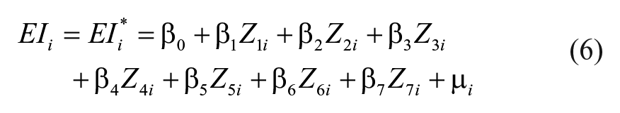

where i indicates the ith cotton farmer; EIi indicates the farmer’s technical, economic, and allocative inefficiencies scores;
Results and Discussion
Average Cost of Cotton Production Rupees Acre−1
Table 2 presents the average variable cost of cotton production for large, medium, and small cotton growers. Total variable cost acre−1 was noted to be highest for small farmers with 63,819.59 PKR/acre followed by large and medium farmers with 62,192.6 and 59,337.38 PKR per acre, respectively. The small farmers in the project area paid more as compared to large and medium farmers, especially for land preparations, seed purchase, stick uprooting process, and irrigation charges. Moreover, small farmers also paid more labor cost incurred in watercourse lining, fertilizer applications, hoeing, and ridging.
Total Cost of Production Rs. Acre−1 for Cotton.

Note. Author’s tabulations.
The findings of the present research are in line with other studies; for example, Ahmad and Afzal (2018) reported that per cost of cotton production was 71,898 PKR per acre in Rahim Yar Khan. The study carried out by Tzouvelekas et al. (2001) in Greece also indicates similar results.
Economic Analysis of Cotton Plantation
Table 3 depicts the per acre economic analysis of the cotton cultivation in the project zone. The results indicate that on average the medium farmers received highest price of 3,543.34 PKR/40 kg with highest yield of 30.47 40 kg acre−1.
Acre−1 Economic Analysis of Cotton Production.

Note. DEA = data envelopment analysis. PKR represents the Pakistan rupees.
Author’s tabulations.
The medium farmers had the highest revenue (103,897.16 PKR/acre) followed by large and small farmers with 109,463.64 and 103,897.16 PKR/acre, respectively. Moreover, the benefit–cost ratio (BCR) was noted to be highest for medium farmers (1.25) and lowest for small farmers (1.02). The results in Table 3 state that small farmers were getting 1.02 by investing 1, whereas the medium farmers were getting highest return of 1.25 by investing 1, which clearly means that small farmers were most vulnerable group with lowest value of BCR, net income, and gross margin.
Descriptive Statistics and the Variables for DEA
Table 4 describes the variables used for efficiency estimation in DEA. The findings of the study indicate that the input application varies across the sample due to different financial conditions of the cotton growers. The statistics reported in Table 4 shows that the average yield of cotton is noted to be 63.18 mounds. In monetary terms, on average, the revenue of cotton farms is found to be 108,240.11 PKR. The average land rent PKR 24,402.50 was paid for 6 months. Other variable costs such as farm machinery, seed, irrigation, fertilizers, and chemical cost are noted to be 4,583.75 PKR, 2,770.00 PKR, 7,486.33 PKR, 7,402.08 PKR, and 4,427.33 PKR, respectively. Cotton plantation and picking is considered as a labor-intensive crop and cost of labor hired for different farm operations is noted to be 9,674.54 PKR.
Descriptive Statistics of the Variables used in DEA Model.
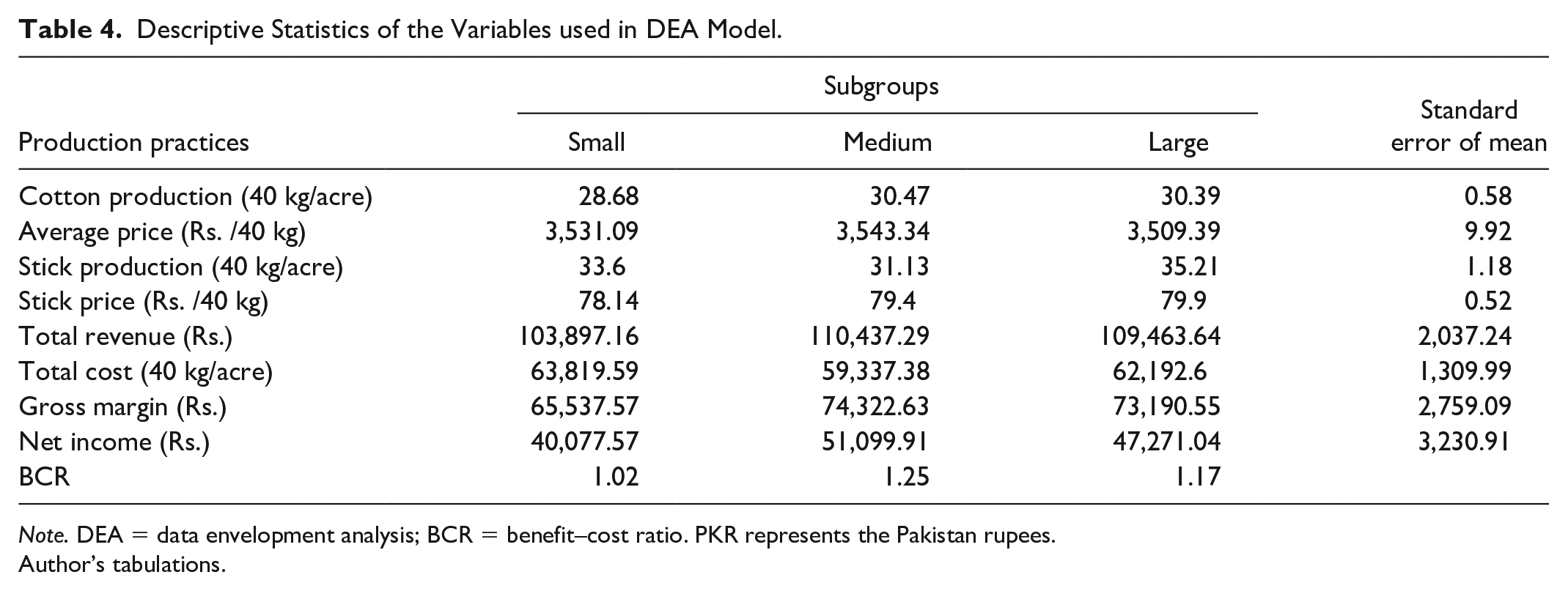
Note. DEA = data envelopment analysis; BCR = benefit–cost ratio. PKR represents the Pakistan rupees.
Author’s tabulations.
Efficiency Distribution
Table 5 depicts the average efficiency scores (i.e., economic, allocative, and technical) were obtained by DEA. The average TE score of cotton farmers was reported to be 95.1%, with maximum 100% and minimum 76.0% efficiency level. These results state that by operating on technical efficient level, the cotton farmers can save about 4.9% of the inputs without affecting the cotton output and keeping the technology unchanged.
Technical efficiency, Allocative Economics Efficiency Distribution.

Note. E stands for efficiency score.
Author’s tabulations.
The findings indicate that 75.83% of cotton farmers were operating above 90% of the technical efficient level. Whereas about 24.17% of the farmers were noted to be technically inefficient and were working between the TE level of 70% and 90%. The average score of EE of cotton farmers is noted to be 66.3%, with maximum 100% and minimum 33.6%. These findings state that about 33.7% of the EE of the farmers can be improved by keeping the output and technology unchanged. There are only 7.5% of the farmers who were above 90% economically efficient, whereas 82% of cotton farmers had less than 80% of EE level. These findings reveal the vulnerability of the cotton growers in the project zone. The AE score of the cotton farmers on average is 69.6%, with maximum 100% and minimum 40.1%. These findings state that cotton farmers can reduce the cost up to 31.4% by improving the allocation of the inputs.
Efficiency Distribution With Respect to Farm Size
The results in Table 6 reveal that TE score was highest (95.5%) for small farmers followed by large and medium farmers with 94.3% and 94.1%, respectively. The AE score reported to be highest for small farmers followed by the large and medium farmers. The EE of the large farmers were noted to be 67.3%, whereas for medium and small cotton farmers the EE were noted to be 62.6% and 62.3%, respectively.
Average Efficiency Distribution and Farm Size.
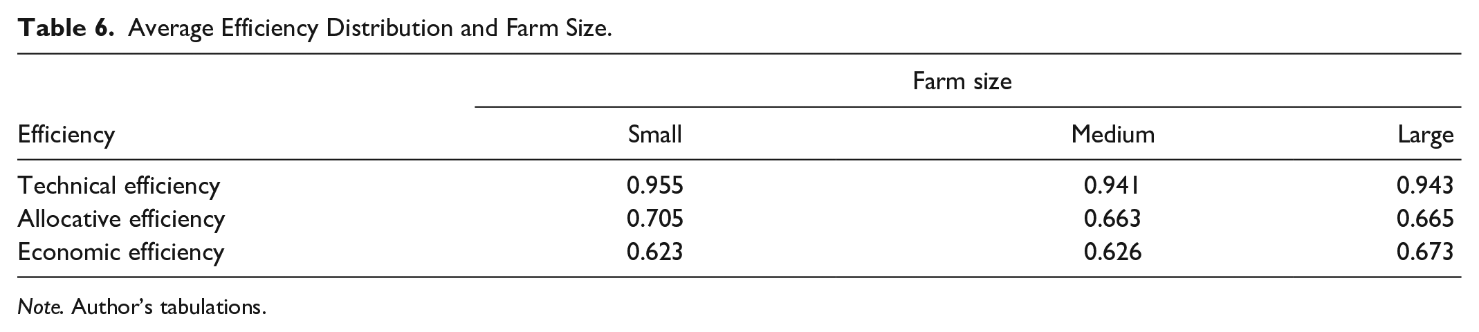
Note. Author’s tabulations.
The EE of the small and medium farmers is an important indicator of farmer financial conditions as the majority of the farmers belong to the small farming group in Pakistan (Faisal et al., 2018).
Variables for Tobit Regression and Descriptive Statistics
Table 7 presents the descriptive statistics of socioeconomic factors affecting farmer’s technical, economic, and allocative inefficiencies. The results state that average age of the cotton farmers was 41.14 years, with maximum age of 65 years and minimum age of 17 years. The education of the farmers is also presented in Table 7, and it is noted that average years of schooling was only 5.72 years with maximum 16 years of education to minimum no formal education. The years of farming experience can be another important factor of farmer’s efficiency. It was noted that average farming experience was 16.87 years with maximum 40 years of experience to minimum 3 years. The average land under cotton plantation was 5.57 acres in the project zone. The distance from the market was noted to be 26 km maximum, with an average of 8.78 km. The availability of agricultural credit and access to agricultural extension services also plays an important role in achieving efficiency; therefore, these two dummy variables were also added into the model to evaluate the factors affecting cotton farmer’s efficiency.
Descriptive Summary of Variables for Tobit Regression.

Note. Author’s tabulations.
The Factors Affecting Efficiency of Cotton Growers
The Tobit regression was applied to evaluate the factors affecting farmer’s inefficiency. The findings of the study presented in Table 8 show that coefficient of age was negative and significant for technical, economic, and allocative inefficiencies. It divulges that farmers with older age were less inefficient as compared to the young cotton growers. Similarly, the experience of the cotton farmers was an important factor of inefficiency on cotton farms, and the experienced cotton growers were less inefficient as compared to the farmers with less experience of cotton plantation. The education factor was also included into the model and it shows that the coefficient of education is significant and negative. It states that education of the farmers can play an important role to reduce farmer’s production inefficiencies. The coefficient of the land under cotton plantation was significant and negative for economic and allocative inefficiencies, which means that farmer’s inefficiency level was decreasing with the increase in land under cotton production. The distance from market was added into the model to investigate the farmer’s incentives and the coefficient of this factor is positive and significant for technical inefficiency; it indicates that as the distance of farm from market increases, the farmers become more inefficient.
Factors Affecting Inefficiency in Cotton Production.

Author’s tabulations.
Extension services includes access to any of the public or private extension services. Private extension services is usually provided by the private agro-based companies, that is, Seed Companies, agro chemical companies, and it may also include nongovernmental organizations (NGOs).
Represents 1% significance level, and β shows coefficient.
Moreover, two dummy variables, that is, access to agriculture credit and availability of extension services, show the significant and negative results, which means farmer’s economic, technical, and allocative inefficiencies level can be reduced by providing them with the easy access to agriculture credit and farm assistance. The agriculture extension services are also very important factor to reduce farmer’s technical, allocative, and economic inefficiencies.
Discussions and Validation
Although cotton cultivation is a profitable process, the small cotton farmers are most vulnerable group and they are earning the least as compared to large and medium farmers, and these results exhibit the similar trend as the findings of the other researchers such as Abid et al. (2011), Kousar et al. (2006), and Mohammad (2009). The average TE in this study was noted to be 95% which is close to the results presented by Faisal et al. (2018). The findings of the Tobit regression model in this study show that education has a significant positive impact on farmer’s production efficiency and these results can be justified with previous literature (Akhtar et al., 2019; Faisal et al., 2018; Ibekwe & Adesope, 2010; Javed et al., 2009; Khan & Ali, 2013; Khan et al., 2017; Naseem, 2018). The results also reveal that cotton farmer’s technical, economic, and allocative inefficiencies can be improved by improving extension services and easy access to agricultural credit, and these findings are also comparable with the existing studies such as Bozoğlu and Ceyhan (2007), Faisal et al. (2018), Hameed and Salam (2014), and Khan and Ali (2013).
Conclusion
The majority of the farmers are small farmers in Pakistan, and the small cotton growers have the most vulnerable economic conditions. The reasons behind low average cotton production and low economic gains were low formal education, lack of access to extension services, expensive farm machinery, and complicated agricultural credit facility to the farmers. Due to the lack of formal agricultural credit services, the small farmers were forced to purchase inputs at expensive rate from informal credit sources. On the other hand, the study found that large and medium farmers were comparatively more efficient than small farmers due to better financial conditions, owned tube well and farm machinery. The economics analysis of the cotton producers shows that small farmers were paying highest cost of cotton production acre−1 due to high irrigation cost, rented machines, costly fertilizers, and overwhelmed application of chemicals to combat the insect and pests and the diseases. The cost–benefit analysis also indicated that the small farmers were getting least return from the investment.
The results in the study show that all the inputs contributed to the cotton productivity. The labor, fertilizers, and chemicals had the highest share in cost of cotton production for all groups. The impact of socioeconomic factors on economic, allocative, and technical inefficiencies exhibits that besides formal education, agricultural credit, and extension services the farm distance from market also had a significant impact on farmer’s inefficiencies. Thus, to address farmers’ low economic incentives, the government should pay key attention to development of infrastructure. Moreover, government should introduce some informal online markets and provide farmers with trainings to sell the produce online to the buyers. The agriculture regulatory authority should regulate the input prices, whereas the quality control department should monitor the quality of inputs, that is, chemicals, fertilizers, and seeds. The provision of technical education, low markup credit facility, and extension services by public and private sector remain the key factors to increase the farmer’s existing low economic incentive.
Concluding that the study finds that socioeconomic characteristics, that is, agriculture credit, extension services, formal education, experience, age, and farm distance are the main reasons of low technical, economic, and allocative efficiencies, farmers are getting less cotton yield, generating less revenue, and getting less returns on investment. These low economic incentives are the most important reason of farmer’s decision to quit the cotton plantation.
However, this study provides with key insights for policymakers to stop farmers from quitting cotton plantation by suggesting how to enhance farmer’s efficiencies? And how to increase farmer’s economic incentives? But, this study did not consider the economic incentive from the competing crops in the analysis, which is the main limitation of the study. Therefore, the future research is planned to evaluate the impact of competing crops’ economic incentives on farmer’s decision of quitting cotton plantation.
Footnotes
Appendix
District Wise Area Under Cotton Cultivation (“000” Acres).

| Sr. no | District name | Area under cotton Acres 2016–2017 | Area under cotton Acres 2015–2016 | Area under cotton Acres 2014–2015 |
|---|---|---|---|---|
| 1 | Bahawalpur | 598 | 675 | 691 |
| 2 | Bahawalnagar | 509 | 542 | 590 |
| 3 | R.Y. Khan | 419 | 511 | 542 |
| 4 | Lodhran | 373 | 484 | 492 |
| 5 | Khanewal | 351 | 465 | 472 |
| 6 | Multan | 349 | 405 | 360 |
| 7 | Muzzafargargh | 336 | 360 | 350 |
| 8 | Rajan Pur | 334 | 350 | 355 |
| 9 | Vehari | 286 | 470 | 515 |
| 10 | D.G. Khan | 180 | 234 | 270 |
| 11 | Sahiwal | 138 | 212 | 199 |
| 12 | Mianwali | 119 | 135 | 143 |
| 13 | Layyah | 106 | 111 | 133 |
| 14 | Bhakkar | 73 | 109 | 118 |
| 15 | Jhang | 68 | 95 | 88 |
| 16 | T.T. Singh | 60 | 92 | 105 |
| 17 | Pakpattan | 59 | 108 | 127 |
| 18 | Faisalabad | 46 | 73 | 75 |
| 19 | Okara | 41 | 55 | 50 |
| 20 | Sargodha | 13 | 17 | 20 |
| 21 | Kasur | 13 | 23 | 28 |
| 22 | Khushab | 6 | 8 | 3 |
| 23 | Chiniot | 4 | 4 | 6 |
| 24 | M.B. Din | 2 | 2 | 3 |
| 25 | Jehlum | 1 | 1 | 1 |
| 26 | Sheikhupura | 1 | 0 | 1 |
| 27 | Nankana Sahib | 1 | 0 | 2 |
| 28 | Attock | 0 | 0 | 0 |
| 29 | Rawalpindi | 0 | 0 | 0 |
| 30 | Islamabad | 0 | 0 | 0 |
| 31 | Chakwal | 0 | 0 | 1 |
| 32 | Gujrat | 0 | 0 | 0 |
| 33 | Sialkot | 0 | 0 | 0 |
| 34 | Narowal | 0 | 0 | 0 |
| 35 | Gujranwala | 0 | 0 | 0 |
| 36 | Hafizabad | 0 | 0 | 0 |
| 37 | Lahore | 0 | 0 | 0 |
Source. DOA (2019).
Declaration of Conflicting Interests
The author(s) declared no potential conflicts of interest with respect to the research, authorship, and/or publication of this article.
Funding
The author(s) received no financial support for the research, authorship, and/or publication of this article.