Sage Journals: Discover world-class research

Abstract

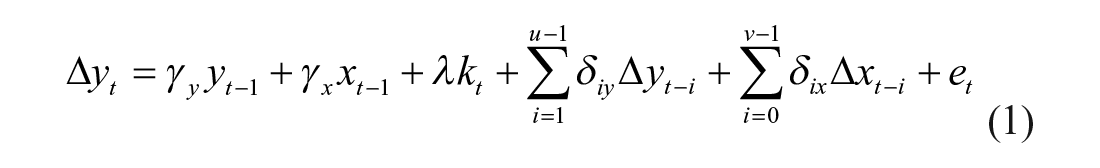
This study analyzed the asymmetric effects of financial development on economic growth using a model augmented with inflation and government expenditure asymmetries to inform model specification. The research question used entails, Do their asymmetry changes significantly influence growth? Using the nonlinear auto-regressive distributive lag (NARDL), the most significant results posit that positive shocks in financial development in the short run and its negative shocks in the long run increase and decrease economic growth, respectively. Regarding inflation, its positive (negative) shocks in both runs, respectively, reduce (increase) economic growth. In comparison, positive shocks in financial development that spur growth in the short run and negative shocks in financial development (government expenditure) that increase (reduce) growth are the most domineering effects as the rest of the shocks insignificantly affect growth. Results clearly demonstrate to an environment steered by stable and sustainable inflation that regulated government expenditure and comprehensive financial system deepening would positively cause economic growth. Therefore, appropriate policies that favor low inflation and reduced government spending, expansion of feasibly reformed financial institutions, capital accumulation, and increased resource mobilization should be instituted if real growth is to positively happen.

Keywords

asymmetries financial development nonlinear auto-regressive distributive lag economic growth

Introduction

The contribution by financial development to economic growth has proven considerably worthy and together with the causalities amid them has too been prudent in understanding the economic growth paradigms. Equally, their asymmetric influence on growth is also essential because of their significant contributions to specific policy formulation and in case of macroeconomic volatilities. Although there exist an overwhelming number of studies on the growth–finance nexus, they have mostly been regional, whereas those on the Eastern region of Africa are very scarce, and unfortunately some have posited confounding results. In addition, with respect to the nonlinear contributions by finance to growth, due to the few existing ones yielding inconclusive results, they are yet scarce. In Kenya, these studies are infrequent, whereas perplexing results have been noted by those that have analyzed the finance–growth nexus and in fact been symmetric. To be specific, they have tumbled on the macroeconomic nonlinearities to economic growth. In the same way, this article investigates how the nonlinearities by financial development affect economic growth using some well-known financial growth indicators.

In most emerging economies, and in search of a self-sufficient and developed financial system, financial reforms have basically been embraced. This confirms to the idea that real growth endowed with efficient financial systems cannot be delinked from economic reforms (Hermes & Lensink, 2003); not forgetting such reforms principally constitutes financial liberalization.

Initially, Kenya’s financial systems had been closed and internally controlled by the government for a long time even in the post independence period. In-ward-oriented trade policies dominated the economy until 1984. Regulated interest rates and credit maximums, restricted access to the banking sectors, limited autonomy of the central and commercial banks and other financial institutions, and controlled interborder trade and capital outflows were characteristics of the long depreciated real growth of the economy in the period before early 1980s. Interest rates rooted on fixed minimum savings and lending rates in the case of credit acceptance and fixed lending rates for credit and loan lending institutions, respectively (Odhiambo, 2009b). Policy makers then followed the Keynesian and neo-classicist idea that low interest rates fundamentally attract investments, leading to financial development and real growth. Thus, a borrower-friendly low interest rate policy that, however, attracted investments guided the financial systems. The policy in turn limited real interest rates that discouraged investors and partly deteriorated financial activities. The result proceeded with government increasing the minimum lending and saving rates by 1% and 2% in that order in 1974 (Kariuki, 1995; Odhiambo, 2009b). However, this did not cause the desired growth as negative externalities from import shocks and delicate economic restructurings in the 1970s and 1980s were unavoidable. The oil crisis of 1973−1974 and 1979, coffee boom of 1976–1977, and the collapse of East African Community in 1978 consequentially accounted for the thrilling impacts on the economy characterized by constant shilling devaluations and inelastic financial rates (Musila & Yiheyis, 2015). Although the mid-1980s appeared to partially favor growth, some reforms such as liberal trade policies, tariff reduction, and elimination of nontariff barriers still savaged real growth. For instance, the persistent high inflation that devaluated currency coupled with the fragility of international trade due to unsound free-floating policies considerably destabilized the outlays by both imported intermediate goods and inputs while causing economic disharmony.

Thus, in 1991 pronounced financial reforms were introduced by the International Monetary Fund (IMF) and the World Bank. From their perspective, reducing government expenditure on socioeconomic services, nominal interest maximums, imposed control on credit allocations and disbursement, and high reserve requirements tied to them restricted real growth through diminishing financial systems as was the case. This marked the remarkable onset of intense and robust structural adjustment programs than during the period 1970 to mid-1980s. In that line, loans credited to the government footed its debts; however, with the imported implied policies (due to IMF and World Bank), they restricted government spending on socioeconomic services at the expense of economic production. Although globalization and informal economy materialized, negative externalities still proceeded, among them being massive unemployment, declined socioeconomic activities, and scarcity of public utility goods and services. In the wake of these reforms, financial liberalization took center stage. In the financial sector, reforms aimed at developing the efficacy of market-based financial systems and revitalizing their competitiveness in the case of foreign markets.

Therefore, specific programs instituted in the sectors include price decontrol in the domestic market, market integration, and privatizations of public assets with some state-owned institution (i.e., commercial banks for self-governance), together with liberalization of global trade and interest rate deregulation. Interest rates since 1982 were fully liberalized in 1991 (Odhiambo, 2009b), resulting in an upward trending interest rate as the 1994 free-floating rate in financial markets attracted positive externalities.

In the banking sector, revamping of credits and monetary mechanisms to undo interest and credit maximums (Jalil & Feridun, 2011) done to date perhaps heightened the autonomy of the central bank’s leverage to normalize systems of accounting and auditing as the finance sector unwrapped to global markets. This has resulted in what can categorize the country’s financial systems as bank-oriented where almost all financial intermediation activities are expedited by banks and related institutions (Demirgüç-Kunt & Levine, 1999). To date, the financial sectors can be seen in two sections: stock market and banking (Nyasha & Odhiambo, 2017), which designates to the financial markets and financial intermediaries, respectively. However, the chief financial processes are still controlled by the banking sector led by the Central Bank of Kenya. Therefore, reforms in the stock market caused its growth from less than 9% in 1980 to more than 49% in 2006 to close to 40% in 2012 (Nyasha & Odhiambo, 2017).

Currently, the economy is market-oriented with liberalized trade systems, with few infrastructure and enterprises owned by the state and sophisticated financial systems. This has resulted in the country’s capital market being the leading stock market in East Africa and among the top five stock markets in sub-Saharan Africa. The banking sector also has grown considerably as evidenced from their increased levels of asset, capital, and deposit accumulation and increased bank credit to private sector leverages. In addition, the liberalized economy has perhaps attracted foreign direct investments (FDIs) which have remarkably instituted capital accumulation, expanded trade to global borders, increased information and communication technologies (ICT) development, and facilitated technological inflows and spillovers to boost the domestic credit and balance of payments (Kinuthia & Murshed, 2015; Odhiambo, 2009a).

In this line, it is imperative to develop a stable and effective financial system. They are critical prerequisites for diffusion of affirmative technological spillovers, capital, labor, and other direct investments that enhance the absorptive capacity in the case of foreign investments (Hermes & Lensink, 2003). Efficiency of these systems is also known to foster capital accumulation through increased domestic investment rates (Calderón & Liu, 2003) and provision of auditing services to investments, thus boosting growth.

In most developing countries like Kenya, investment reforms are imminent to suffice the normally competitive foreign markets. Consequently, there would be unrelenting risks due to technological entrepreneurial shifts and upgrading from the incumbent barrel to foreign technologies. Buffering such risks would only require an outstanding financial system if they are to remain competitive in the case of external shocks in the stock markets or other financial institutions (Batuo et al., 2018; Hermes & Lensink, 2003). However, the risks are further worsened when financial liberalizations become weak or respond nonlinearly. Perhaps the instituted financial liberalization has spurred development in the country.

However, the progress by such financial developments has also been pro-cyclical with economic downturns harming financial systems during recessionary periods. At this moment, externalities emerging from financial liberalization would negatively deter real growth, which is a common case for low and emerging states. Consequently, there would be imminent capital outflows inducing currency volatilities. According to Batuo et al. (2018), financial crisis recurrence, as for the case with most low-income states, is a clear indicator of the inefficacy of existing models of human and market behaviors in averting the constantly lingering risks and uncertainties that continually destroy real growth. Similarly, today’s post-reform economic downtowns prevalent in Kenya are the repercussions of some impotent incumbent financial development policies. The policies have destabilized the sector, which can be manifested through volatilities in asset pricing and diminishing market liquidities, and as the economy through real productivity is correlated with financial sectors (Batuo et al., 2018; Nyaranga et al., 2019) has generally been demeaned.

In the literature, a large number of studies have reviewed the symmetric growth–finance association and reported confounding results or missing relationship (Atindehou et al., 2005; Deltuvaitė & Sinevičienė, 2014; Kar et al., 2011; Kinuthia & Murshed, 2015; Klobodu & Adams, 2016; Ujunwa & Pius, 2010). Others reported significant finance–growth relationship (Adeniyi et al., 2015; Batuo et al., 2018; Jalil & Feridun, 2011; Kinuthia & Murshed, 2015; Levine, 1997; Nyasha & Odhiambo, 2017; Odhiambo, 2009a, 2009b; Rousseau & Vuthipadadorn, 2005; Sobiech, 2019) and imply that the debate on the contributions by finance to growth is still open.

It is clear that most of these studies have concentrated on the relationship between and/or the impact of financial development on economic growth. Results have been inconclusive or invariant due to either inappropriate estimation techniques that diverge from the data-generating processes or improper choice of the proxies of financial developments. Furthermore, a section of the aforementioned studies has considered cross-sectional or panel data (Calderón & Liu, 2003; Hermes & Lensink, 2003; Tsagkanos & Siriopoulos, 2015).

In addition, studies investigating the nonlinearities on finance–growth nexus and/or their proxies are still inconclusive (Fousekis et al., 2016; Katrakilidis & Trachanas, 2012), regional-based (Anderson et al., 2014; Ehigiamusoe et al., 2019; Tsagkanos & Siriopoulos, 2015), and regime-based, mainly underscoring emerging/emerged markets (Dinh Thanh & Canh, 2019; Tsagkanos et al., 2019), as those exploring the finance–growth linkage in developing countries are still largely missing. Furthermore, cross-sectional-based studies have demonstrated results that are far much general than informing the normally country-specific details as they fail to suggest specific policies to a country’s specific economic growth. This is against the backdrop of increasing concerns of asymmetric impacts on macroeconomic variables to appropriately inform sound policies in such developing nations. Although nonlinearities in financial deepening importantly affect growth in Kenya, such studies as well are still very scanty, and not forgetting the relentlessly instituted strategic financial reforms in the previous decades credibly have altered the asymmetric effects on the general growth of the economy in the country, and this requires demystification.

This article devotes to bridging the aforementioned gap to appropriately inform specific policies of sustainable economic growth and financial system integration relative to government spending and inflation. We explore how the asymmetric changes in financial development and the two control macroeconomic variables affect growth to trace how sustainable economic growth might alleviate the continually persistent unemployment and lagging inflation that destroy the well-being of citizens. To the best of our search, limited research works have expedited the real growth–financial development relationship in Kenya (Kinuthia & Murshed, 2015; Musila & Yiheyis, 2015; Nyasha & Odhiambo, 2017; Odhiambo, 2009a, 2009b) and unfortunately have also reported mixed results. Also the pooled effects of government expenditure, inflation, and financial development on economic growth in the case of Kenya are still limited, but if any studies exist, they have not explored their normally important asymmetries on real growth. This is because, empirically, the weight of positive and negative shocks on the target variable (economic growth) by financial development is normally dissimilar. We devote to address this gap.

This article is profoundly different and adds to the literature in many ways. First, the authors innovatively employ the principal component analysis (PCA) technique and conceive a composite financial deepening indicator using typical determinants of financial development. Second, we employ the NARDL that permits inflation, financial development, and government expenditure to be decomposed to positive and negative partial sum of squares, and their effects are observed on growth. Still, addition of inflation and expenditure in the process is to supplement studies that only incarcerate financial development and overlook the important effects of control proxies. Third, their dynamic multipliers allow us insight into how their asymmetric shocks impact growth as they respond to the newly found long-run equilibrium from previous disequilibrium dynamics. The most critical outcomes noted in this study are that, first, the growth–finance relationship is asymmetric. Second, in the short run, increasing financial development increases growth, and in the long run, reducing (increasing) economic growth rapidly responds to slump in financial development (an increase in government expenditure).

The rest of the article is designed as follows. Section “Literature Review” reviews the literature, section “Empirical modeling” presents the data and methodology, section “Empirical Results and Analysis” presents the results and discussion, and section “Conclusion” concludes and forwards some guideline policies for sustainable economic growth in Kenya.

Literature Review

Literature widely documents that financial developments via appropriate financial systems facilitate accumulation of capital and boost credit availability while causing growth. Levine (1997), therefore, points out various conduits that financial development affects growth, that is, via improved exchange of goods and services, enhanced capital accumulation and allocation, managing human resources and cooperate governance, decontrolling interest rates, mobilizing savings, and controlling the risks to finance. This implies that higher capital accumulation steers investments and savings, which, in turn, strengthens the scale and intensity of economic activities as real growth materializes (Nyasha & Odhiambo, 2017). Similarly, a well-developed financial system that is technologically sound ably causes, among them, efficient capital mobilization and allocation, minimizes information skewness and transaction costs, minimizes risks, and avail funds for private investments while causing growth (Bencivenga & Smith, 1991; Solow, 1960). Hence, financial developments are consequential in influencing economic growth, with the level of influence dependent on the efficacy of underlying financial system development.

Literature contains a large number of studies analyzing the contribution made by financial development to economic growth; however, their reported findings are still confusing and render the relationship inconclusive and still debatable. Similarly, studies investigating the asymmetric impacts of financial developments on economic growth, either way or from growth to financial development, are very uncommon. Although if any, they still have posited perplexing results, posing their nonlinearity in contributions to real growth to further arguments and/or denting the dire need of the knowledge of nonlinearity effects by such macroeconomic variables on economic development. However, irrespective of the scanty asymmetric finance–growth nexus and country-specific studies for lower-middle-income countries and rest of the economies, the literature comprehends some empirical works that have attempted to study the finance–growth relationship.

Initial studies in this area noting the significant contribution of financial development to growth were pioneered by Schumpeter (1911) and seconded by Patrick (1966) who reported the growth–finance relationship based on three assumptions, that is, supply-led, demand-led, and stage of development hypothesis. In supply-led assumption, financial system deepening heightens growth and implies correctly designed financial market reforms support efficacy with which capital is accumulated and invested, yet boosting growth (Calderón & Liu, 2003; Levine et al., 2000). For demand-led assumption, productive economic growth stimulates and attracts financial development and is tied to the innate reaction by financial development, and specifically when implemented, structural reforms facilitate production and finally boost the necessary structures which favor financial system development to befit the growing economy. The “development stage theory” portrays a development shift between supply-led and demand-led assumptions, finally resulting in the growth of economy and financial systems in the long run. That is, initially the properly functioning economic growth boosts production and provides the necessary structures that enhance financial system integration and development (the demand-led assumption dominates). With such financial systems, for instance, they attract foreign capital inflows, and new skills and technologies via liberalization and improve their leverage to pay back to economic growth as supply-led growth happens (Calderón & Liu, 2003; Patrick 1966). The third hypothesis is indeed interesting as the backdrop creates room for investment and financial consolidation with a general growth in economy.

With these insights, previous studies have postulated mixed findings regarding the finance–growth causality as unidirectional (supply- or demand-led), feedback, or no causalities. We delve into some of these works and initiate a unidirectional causality which is either finance-led or growth-led. That is, by the former, integrated financial system deepening improves sector growth, whereas by the latter, new financial system deepening quenches the demand created by the initially grown economy (Patrick, 1966). Abu-Bader and Abu-Qarn (2008a) from the North African and East Asian panel reported significant supply-led growth in Tunisia, Algeria, Morocco, and Egypt and weak growth-led effects in Israel. In Kenya, based on how a finance–interest rate linkage affects growth, Odhiambo (2009a) found that interest rate liberalization heightens financial deepening, with efficacy level determining their scale of heightening as economic growth is also boosted by financial deepening. The findings confirm the requirement for robust interest reforms for positive growth. A similar case study is reported by Nyasha and Odhiambo (2017), but with market-based financial systems they increase real growth unlike bank-based systems. As the socioeconomic status via the level of economic activities by the society also plays a role in providing the necessary market for utility of and attraction of financial systems, Khemili and Belloumi (2018) explored this aspect using inequality and poverty levels to economic growth for Tunisia and reported significant long-run feedback causality from poverty to inequality and as growth granger-causes poverty. This means that to increase the economic leverage of the people that boosts investments, demand, and general income of the people, policies which reduce poverty and offset the inequality gap and boost growth should be implemented while demand-led growth happens.

Kinuthia and Murshed (2015) comparatively show an FDI supply-led growth in Malaysia, which is missing in Kenya. These results point to the missing proficient financial system reforms and foundations that provide an equilibrium FDI attracting environment in Kenya compared with Malaysia. Furthermore, and still based on data from Kenya, Musila and Yiheyis (2015) still posit mixed consequences using both policy and aggregated trade openness. By the former, trade openness reduces both investments and growth; by the latter, trade heightens investments, but the effect on growth is missing. An important note also is variabilities in trade through its positive effects on host country foster growth. Tsagkanos and Siriopoulos (2015) expedite the stock market relationship with industrial production based on threshold cointegration model for Eurozone and report significant findings. The long-run adjustments between stock price and industrial production are asymmetric for southern Eurozone due to weak structural competitive foundations compared with northern Eurozone which experiences symmetric adjustments. Adeniyi et al. (2015), based on a Nigerian-based data set spanning from pre- to post-reform periods, report befuddling supply-led correlation in all periods. The hypothesis has a negative impact at normal finance growth level but is positive when the squared level of finance depth indicator is included, and this concludes that development is dependent on the threshold of financial service development.

Batuo et al. (2018), on a relationship mission between financial variables and growth to account for the post-2008 financial crisis in Nigeria, find interesting results. First, financial liberalization and deepening that boost financial instability are finally reduced by economic growth in the periods before liberalization. Tsagkanos et al. (2019) explore the two newly found theories regarding relationship amid FDI and stock market development for the period 1984–2014 which are differentiated based on two markets—emerging market until 2001 and developed country since 2002 while employing both cointegrated and Markov switching techniques for the Greece data set. They find that when using cointegration and Markov regression, there is a symmetric long-run linkage with weak positive effects between the full sample, strong linkage in the emerging market, and insignificant linkage in the developing nation. Sobiech (2019), with a generalized method of moments (GMM) technique on a data set of developed and emerged markets and remittance inflow based on financial indicator, reports a significantly positive supply-led growth in developing countries than emerged markets, with greater long-run weight for the countries in the developing set. Ehigiamusoe et al. (2019) also report mixed findings that growth boosts financial development in middle- and high- income countries, but regarding the high inflationary states, inflation is detrimental to financial developments. Other studies include

Regarding feedback causality, we find them in studies such as Odhiambo (2009a) on a Kenyan data set, but with weak causality weights, and Abu-Bader and Abu-Qarn (2008b) on an Egyptian data set that corroborates positive finance–growth feedback among others. Also, the missing causalities might be implied either way by many studies on the prevailing temporal finance–growth relationship as incongruence. This implies that the factors determining the growth in financial systems are implicitly rooted in financial reforms, whereas those causing economic growth are by actual factors (Graff, 1999). The findings from the studies by Atindehou et al. (2005) in West Africa for missing finance–growth linkage support Lucas’s (1988) critique that the finance causes growth and vice versa is an illusory correlation, and thus, linking financial deepening to cause growth might be exaggerated. A similar observation is made by Kar et al. (2011) in Middle East and North Africa (MENA) and missing linkage linked to the different country-specific infrastructural foundations with different profound scales of development. Deltuvaitė and Sinevičienė’s (2014) findings add to this.

Generally, the supply-led theory has largely been explored than the demand-led theory and/or reported missing causality when some were analyzed based on nonlinear frameworks and either on time series or panel data sets. Also, some have been using linear techniques and analyzing the symmetric nature of finance–growth using either linear cointegrating methods such as auto-regressive distributed lag (ARDL), vector autoregressive (VAR), and vector error correction model (VECM) or non-cointegrating methods such as the ordinary least squares. Few have delved into the asymmetric side but have been mainly regional-based like Tsagkanos and Siriopoulos (2015) and Ehigiamusoe et al. (2019), among others. The current work is concerned with the asymmetric impacts of financial development on growth to exploit the specific policy that supports increasing productivity and financial growth. Although linear studies on growth–finance in Kenya exist, this study is one of its kind. We show that finance asymmetrically affects growth and so does inflation and government expenditure. Our work contributes to literature in findings, way of approach, and filling the gap by missing studies.

Empirical modeling

Data

The data set contains annual data ranging from 1972 to 2017 concerning macroeconomic variables in Kenya from the World Bank (https://data.worldbank.org/). They include gross domestic product (GDP) calibrated in constant US$, inflation rate as the GDP deflator, government expenditure as the sum of final consumption expenditure in constant US$ weighted using GDP, and financial development depth indicator still constructed with variables from World Development Indicators (WDI), that is, broad money as the share of GDP, domestic credit as credit awarded to private sectors by commercial banks weighted by GDP, real interest rate as deviation between lending and inflation rates, and trade openness aggregated from cumulative sum of exports and imports weighted by GDP and calibrated in constant 2010 US$.

The function of GDP is to designate economic growth and inflation to seize the extent of macroeconomic instability to finance via the impact on money components and general economic activities. For instance, high inflation on households suppresses investments but fosters consumptive activities so that the level of financial and real growth is in the end affected (Hongo et al., 2019). Government expenditure captures the macroeconomic influence by the state in provision of public goods and service while changing the stance of necessary infrastructural developments upon which financial development is activated. What is next concerns how financial development is aggregated.

The literature has pointed to different proxies of financial development, among them being FDI/GDP, market capitalization, stock trade, and domestic credit aggregated by GDP (Narayan & Narayan, 2013; Saci & Holden, 2008). Others preferred financial intermediaries due to feasibility to conduit resources for investors and cooperate governance and provisions of necessary fundamentals in risk management in the banks. Jalil and Feridun (2011) embraced the intermediaries as the proportionate share of commercial bank assets to the cumulative assets owned by central and commercial banks. M2 as the share of GDP has widely been used as it defines the power for intermediary services and leverage by financial systems to provide credit facilities for investment growth (Levine, 1997). Many studies have used the proxy in their finance–growth analysis (Lawrence et al., 2014; Nawaz et al., 2019). Others have utilized liquid liabilities (M3) which demonstrate how the liquidity by banking sector relatively varies and grows over time, and hence the importance of money growth in developing countries as it increases monetization paramount in the integration of financial institutions and successive developments. Saci and Holden (2008) have used the proxy and reported partly promising outcomes. As fixed deposit (FD) is also tied to stock market development, Tsagkanos et al. (2019) implore the real interest rates to incarcerate the stance of monetary policy instruments toward financial system development and partially report mixed results for the different analyses implored. To capture the significance of private sector finances, other studies have successively used the domestic credit/GDP.

In sum, the literature has presented varied proxies of financial development. Unfortunately, they nose-dived to designate a distinct and succinct component of FD, for instance, Hermes and Lensink (2003) linked the efficiency of such proxy to financial intermediation as the criterion for selection. This is explained by the fact that economic globalization has consequently transformed the determining factors of FD to the extreme that the specificity of exact FD proxy is inevitably continually debatable. Furthermore, no singular proxy is banked on to signpost financial developments, and on the contrary, if the above variables are singly incorporated into a common regression, they would induce multicollinearity and spurious regression.

In this line, we constructed a financial depth indicator using some well-resolved proxies—that is, broad money/GDP, real interest rate, domestic credit to private sector per GDP, and trade openness. Broad money is used to capture money supply and capital accumulation while demonstrating the monetary input in the financial sectors. Trade openness incarcerates the influence of globalization that consequentially foster foreign capital inflows and technological spillovers while influencing growth via supply-led effects on financial sector. Domestic credit captures financial transfers to the private sectors and de-gapping M2 and M3 transfers for private investments. Real interest, which partly designates the efforts by monetary policies, depicts the magnitude of inflationary pressure in both financial and economic activities. Its uncertainty distorts the stance of financial systems as growth is caused.

However, to counter the above shortcomings, the authors entrapped the PCA on the variables and derived a succinct depth component of financial development. Why is the preference of the technique twofold? First, it aggregates while minimizing autocorrelations as variable endogeneity might be inevitable in the case of individual incorporation. Second, it sufficiently produces a representative index that still preserves the critical information enshrined in the temporal variables.

Thus, based on the procedure applied and the results presented in Table 1, the correlation matrix in the upper part of the table initiates some correlation among the variables. The pairs trade openness and real interest, and broad money and domestic credit to trade openness exhibit negative correlation, whereas the correlation is positive for the case pair real interest to both broad money and domestic credit. In addition, both weak and strong autocorrelations are obvious amid the variables and conclude that, if all four are pooled into a common regression, the parameters would be spurious in estimation. However, information in this case is representative and sufficient than single indicator would have demonstrated apart from inducing spurious regression.

Table 1.

Financial Development Index Aggregation.

Variable	Real interest	Trade openness	Broad money	Domestic credit
Correlation matrix
Real interest	1
Trade openness	−0.210	1
Broad money	0.429	−0.417	1
Domestic credit	0.384	−0.620	0.8456	1
Component analysis
Component	Eigen values	% variance	Cumulative proportion (%)	First principal component
1	66.300	68.341	68.341	(0.094)^R/Interest
2	26.973	27.810	96.141	(–0.059)^Trd/Op
3	3.649	3.761	99.901	(1.069)^BrdMny
4	0.097	0.099	100.000	(38.24)^D/credit

Note. Numbers in parentheses are estimated coefficient values for respective superscripted variable.

In this line, results in the rear section of Table 1 demonstrate specific derivation by the PCA component, which makes clear that the first to fourth components pose explanatory powers ranging from 68% to 0.1%, which depicts that it is only in the first component 68% variations in FD is accounted for compared with less than 1%. We conclude that the first component bears the highest explanatory power to best accounts for the variations in financial development compared with the rest of the variables and thereafter only present information about the first component. Importantly, to note, the estimates in the fifth column are the ones used to weigh the final FD depth indicator fed into proceeding regression.

Methodology

This section presents the methodology used to delve into the asymmetric effects of financial developments on growth—that is, the nonlinear ARDL of Shin et al. (2014).

However, our empirical specification is initiated from the usual symmetric ARDL model by Pesaran et al. (2001). Therefore, if x and y are a set of bivariate macroeconomic series but without I(2) stationary variables, the ARDL model is written as

Δ y_{t} = γ_{y} y_{t - 1} + γ_{x} x_{t - 1} + λ k_{t} + \sum_{i = 1}^{u - 1} δ_{i y} Δ y_{t - i} + \sum_{i = 0}^{v - 1} δ_{i x} Δ x_{t - i} + e_{t}

(1)

where ∆ is the difference operator, $γ (δ)$ is the long (short) run coefficients, $λ$ is the vector of deterministic regressors regarded as exogenous, for example, trend, and $e_{t}$ is an i.i.d. component.

The first step is testing for cointegration. Thus, equation (1) is said to be cointegrated if x and y postulate along run relationship for a rejected null hypothesis that jointly $γ_{y} = γ_{x} = 0$ or separately $γ_{y} = 0$ and $γ_{x} = 0$ using the Wald test. This results in F- and t-statistics, respectively. Their statistical significance is then bound tested using Pesaran et al.’s (2001) or Banerjee et al.’s (1998) statistical table. The critical bound is a pair of I(0) and I(1) that x and y are level- and difference-stationary, respectively. Furthermore, regarding F-statistics, the variables are cointegrated if the calculated statistics fall above I(1), non-cointegrated if below I(0), and inconclusive for statistics falling between the bounds. The inverse happens regarding t-statistics. The proceeding steps involve identifying the short-run and long-run impacts of x $x$ on y using their p-values.

Why the symmetric ARDL is preferred to multivariate regressions is due to its many advantages over other cointegrating endogenous models.¹ However, we do not discuss the preferences and instead delve into the foundation of the asymmetric method. That is, as with other symmetric regression methods, they assume parameters as inelastic and symmetrically responding to changes in the macroeconomic environment. Similarly, the error correcting term by these methods is assumed to linearly respond to economic volatilities and at constant speeds (Enders, 2014/2015). However, this is not the case if x on y reacts/responds asymmetrically, implying that they differently react to economic forces pooling positively/negatively away from the equilibrium. Also, application of symmetric ARDL would result in inconsistent and nonrobust estimates (Anderson et al., 2014), resulting in mirage policy conclusions. Consequently, in the economic growth policy analysis, it is imperative to acknowledge the prevalence of economic frictions² that significantly contribute to the vertical movements unlike the broad impact on the economy. As a matter of fact, the nonlinear ARDL by Shin et al. (2014) adopted for this purpose sufficiently captures the foretold shortcomings.

The method utilizes the decomposed partial sum of positive and negative squares to investigate the asymmetries by regressors in both runs giving consistent estimates with nonlinearities. Let the economic growth be yt and $f d_{t}$ for financial development. Therefore, to represent this method, equation (1) starts to modify into the following long-run linear asymmetric representation:

y_{t} = β^{+} f d_{t}^{+} + β^{-} f d_{t}^{-} + μ_{t}

(2)

where $β^{+} (β^{-})$ are the long-run coefficients linked to the partial sum of positive (negative) changes in $f d_{t}$ (Shin et al., 2014), integrated by the function $f d_{t} = f d_{t} + f d_{t}^{-} + f d_{t}^{+}$ using the process

\begin{array}{l} f d_{t}^{-} = \sum_{j = 1}^{t} Δ f d_{j}^{-} = \sum_{j = 1}^{t} \min (Δ f d_{j}, 0) and f d_{t}^{+} \\ = \sum_{j = 1}^{t} Δ f d_{j}^{+} = \sum_{j = 1}^{t} \max (Δ f d_{j}, 0) \end{array}

(3)

The linear stationary combination (zt) of (2) and asymmetric partial squares is

z_{t} = k + ϕ_{1}^{+} y_{t}^{+} + ϕ_{2}^{-} y_{t}^{-} + γ_{1}^{+} f d_{t}^{+} + γ_{2}^{-} f d_{t}^{-} + e_{t}

(4)

Stationarity in equation (4) is achieved if z_t = I(0) and with linear asymmetric long-run cointegrating relationship for a rejected null hypothesis $ϕ_{1}^{+} = ϕ_{2}^{-} = β_{1}^{+} = β_{2}^{-} = 0$ . However, the estimated equations (2) and (4) are likely to assume multicollinearity and endogeneity that require to be corrected before cointegration analysis. The dynamic formats of the equations are therefore appropriate in addressing such issues. We therefore write equations (2) and (4) considering their dynamic formats as

y_{t} = \sum_{i = 1}^{p} λ u n_{t - i} + \sum_{i = 0}^{q} (β^{+} f d_{t - i}^{+} + β^{-} f d_{t - i}^{-}) + e_{t}

(5)

where $λ$ is the AR parameter and $β$ is the parameter causing dynamic adjustments with the cointegrating dynamic format, which is represented as

\begin{array}{l} Δ y_{t} = ρ y_{t - i} + φ^{+} f d_{t - i}^{+} + φ^{-} f d_{t - i}^{-} + \sum_{i = 1}^{p} δ_{i} Δ y_{t - i} \\ + \sum_{i = 0}^{q} Δ η_{i}^{+} f d_{t - i}^{+} + Δ η_{i}^{-} f d_{t - i}^{-} + e_{t} \end{array}

(6)

Equation (6) is the NARDL by Shin et al. (2014) where $β^{+} = - φ^{+} / ρ$ and $β^{-} = - φ^{-} / ρ$ reflect the long-run asymmetric coefficients and $δ$ and $η$ the asymmetric short-run dynamics. Equation (6) is cointegrated for a rejected null hypothesis that $ρ = φ^{+} = φ^{-} = 0$ based on F-statistics (Pesaran et al., 2001) or individually, $ρ, φ^{+}, φ^{-} = 0$ (Banerjee et al., 1998) and after rejected nulls $φ^{+} = φ^{-}$ , respectively, that their long-run parameters are valid. The asymmetric short-run dynamics are significant for rejected nulls that $η_{i}^{-} = η_{i}^{+}$ , whereas long-run asymmetries are significant for rejected nulls that $φ^{+} = φ^{-}$ .

Finally, in this faith, we explore how growth would respond in the long run to nonlinearities in financial development after a standard shock. This is the dynamic multiplier useful in expediting the temporal growth behavior as it changes from a backdrop of previous short-run dynamics and initial instabilities to new-found equilibrium after an economic shock in financial development. The multiplier uses the process

\begin{array}{l} m h^{+} = \sum_{i = 0}^{h} \frac{\partial y_{t + i}}{\partial f d_{i}^{+}} = \sum_{i = 0}^{h} β_{i}^{+} and m h^{-} = \sum_{i = 0}^{h} \frac{\partial y_{t + i}}{\partial f d_{t}^{-}} \\ = \sum_{i = 0}^{h} β_{i}^{-} h = 0, 1, 2, \dots, t \end{array}

(7)

in which $m \to \propto$ and $m h^{+} (m h^{-}) \to β^{+} (β^{-})$ where $m h^{+}$ is the long-run asymmetric coefficients.

$m h^{+}$ and $m h^{-}$ are the asymmetric long-run coeffi-cients which achieve consistency as $m \to \propto$ so that $m h^{+} (m h^{-}) \to β^{+} (β^{-})$ . $m h$ is important because it enshrines the crucial information responsible for the volatilities.

However, using only FD to observe its effects on growth will not only produce insufficient results but also the asymmetric model might be misidentified and likely nonrobust. To control these effects, the authors incorporated government expenditure and inflation as they are believed to support economic growth. Government expenditure integrates the economic influence by the state in providing resources for public utility while heightening the necessary infrastructural developments for financial system integration. Inflation captures the inflationary pressure on financial sector via altering the interest rates. Their interactive background holistically offsets/heightens economic growth via the supply-led growth on FD.

Equation (6) is therefore modified using inflation (π_t) and government expenditure ( $g x p_{t}$ ) as follows:

\begin{array}{l} Δ y_{t} = ρ y_{t - i} + φ^{+} f d_{t - i}^{+} + φ^{-} f d_{t - i}^{-} + ϕ^{+} g x p_{t - i}^{+} + ϕ^{-} g x p_{t - i}^{-} + \\ ϑ^{+} π_{t - i}^{+} + ϑ^{-} π_{t - i}^{-} + \sum_{i = 1}^{p} δ_{i} Δ y_{t - i} + \sum_{i = 0}^{q} Δ η_{i}^{+} f d_{t - i}^{+} + \\ \sum_{i = 0}^{q} Δ η_{i}^{-} f d_{t - i}^{-} + \sum_{i = 0}^{q} Δ λ_{i}^{+} g x p_{t - i}^{+} + \sum_{i = 0}^{q} Δ λ_{i}^{-} g x p_{t - i}^{-} + \\ \sum_{i = 0}^{q} Δ γ_{i}^{+} π_{t - i}^{+} + \sum_{i = 0}^{q} Δ γ_{i}^{-} π_{t - i}^{-} + e_{t} \end{array}

(8)

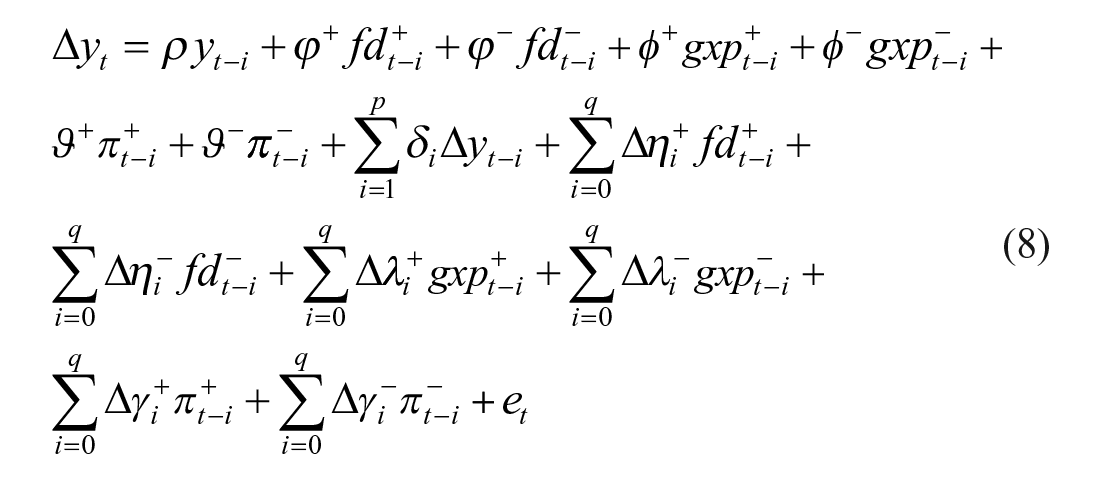
The ordinary least square regression is then applied on equation (8) based on three procedures. First, asymmetric cointegration is tested using the asymmetric restrictions $ρ = φ = ϕ = ϑ = 0$ designating a linearly cointegrated system. Second is validating the long- and short-run asymmetric impacts of FD and other regressors on growth. The long-run asymmetric impacts are given by $- φ / ρ$ , $- ϕ / ρ$ and $ϑ / ρ$ estimated for both positive and negative squares. Third is the exploration of their long- and short-run asymmetries using the asymmetries $φ = ϕ = ϑ$ and $δ = η = λ = γ$ , respectively, for both positive and negative squares as the null hypothesis.³

Preference of the NARDL model in this case than other time series techniques which explore nonlinearities is threefold. They are mostly inferior compared with the NARDL. For instance, the Markov switching regression and threshold regressions (Tsagkanos et al., 2019; Tsagkanos & Siriopoulos, 2015) are the best befitting analyses in shifting regimes, with the former also testing nonlinearities without imploring their vertical movements from the long-run equilibrium changes and both also underperforming on asymmetric long-run cointegration relationship giving nonrobust estimates. It is also infeasible to observe the specific effects of asymmetric correction from previous dynamics via past/future disequilibrium—the probability plot is not sufficient to clearly delineate the specific long-run shock behavior to the asymmetries identified. The NARDL, through this article, therefore accounts for the shortcomings and finds its superiority over such nonlinear techniques. First, it decomposes the regressors into their respective partial sum of positive and negative squares and observes their effects with(out) addition of the dummy incarcerating shifts in regimes while significantly reporting their asymmetric behaviors. Second, it integrates bound testing into the long run and synchronously estimates with the short run while preserving the data-generating processes, resulting in robust estimates. Third, is its ability to investigate the temporal dynamics in growth as it tries to adjust from a backdrop concocted by short-run dynamics and initial disequilibrium to new-found stability (the dynamic multiplier).

Furthermore, estimation of equation (8) is done parsimoniously while shedding off trivial parameters to attain accuracy in estimation and is important in de-noising the dynamic multipliers. An important point to note is that the variables as entered in the regression are initially logarithm transformed to eliminate raw data problems like abnormal skewness and kurtosis and to induce elasticities to growth.

Empirical Results and Analysis

The section initiates from unit root analysis to determine stationarity and is fundamental to exclude any I(2) stationary variable that normally has no odds on the Pesaran bounds. Table 2 displays these results by both Augmented Dickey–Fuller (ADF) and Phillips–Perron (PP) for inflation, GDP, government expenditure, and financial development in their natural logs. Government expenditure and GDP at both tests show difference stationarity, whereas inflation and FD display confounding stationarity. For instance, at intercept only, FD is level stationary unlike at both intercept and trend, but by PP and at intercept only by ADF, inflation is level stationary. Such confounding outcomes are determinable by the different specifications of the test equation and the data-generating process. However, we reach a conclusion that the four macroeconomic variables are mixture stationary without I(2) and proceed for NARDL analysis.

Table 2.

Unit Root Test.

	Augmented Dickey–Fuller		Phillips–Perron
Variable	C	Constant and trend	C	Constant and trend
$y_{t}$	0.315	−1.290	−0.056	−1.562
$f d_{t}$	−0.745	−4.631*	−1.446	−3.515**
$g x p_{t}$	−0.655	−3.129	−0.590	−2.420
$i n f_{t}$	−3.416**	−3.053	−5.270***	−5.343***
$Δ y_{t}$	−4.212***	−4.231***	−4.524***	−4.572**
$Δ f d_{t}$	−6.203***	—	−8.219***	—
$Δ g x p_{t}$	−4.209***	−4.162*	−4.232***	−4.187***
$Δ i n f_{t}$	—	−8.322**	—	—

Note. ∆ is the difference operator, whereas *** and ** indicate 1% and 5% significance. Optimal lag chosen is based on Akaike information criterion.

Regression of equation (8) is done based on an ARDL (1,1,1,1) model automatically chosen from a baseline framework of four lags chosen based on Schwarz and Hannan–Quinn information criterion. The results of the symmetric bound testing done are presented in Table 3 and have the F-statistics (F = 4.942) and t-statistics (t= −4.027) significant at 10%, implying there exists asymmetric long-run cointegrating relationship. Also, by significant cointegration, the variables pooled in the regression are stationary, partly supporting results in Table 2.

Table 3.

Symmetric Bound Test.

			Critical bounds
Statistic		Significance	I(0)	I(1)
F-statistics	4.942^a	10%	3.490	4.450
t-statistics	−4.027^a	10%	−3.130	−3.84

Null hypothesis tested is that the long-run cointegrating relationship is symmetric. The test equation is done at both unrestricted constant and trend using K = 3 (number of regressors fitted in the level regression) and on the Pesaran et al. (2001) table.

Rejection at 10%.

In Table 4, the null hypothesis that the variables in the runs are symmetric is rejected, meaning that both in the short and long run, the positive and negative partial sum of squares are significantly different from each other and support asymmetric behavior. Thus, inflation, financial development, and government expenditure differently influence growth in both runs and with different levels of positive and negative effects. This triggered their further analysis to find their impact on growth.

Table 4.

Test for Symmetries.

Wald statistic	χ² statistic
$W_{SR}$	21.080*** (0.000)
$W_{LR}$	77.573*** (0.000)

Note. The null hypothesis is that the coefficients are symmetric. $W_{SR}$ and $W_{LR}$ denote the short- and long-run Wald statistic symmetries, respectively. $W_{SR}$ is $\sum_{j = 0}^{p - 1} η j^{+} = \sum_{j = 0}^{p - 1} η j^{-}$ and $W_{LR}$ is $- θ^{+} / ϕ = - θ^{-} / ϕ$ . The p-estimates are represented in parentheses.

***

represents the 1% rejection level.

Table 5 demonstrates the nonlinear impacts of financial development, government expenditure, and inflation on growth. Starting with long-run asymmetric impacts and with government expenditure, we read that its negative partial sum ( $g x p_{t - 1}^{-}$ ) is insignificant unlike the lagged positive one ( $g x p_{t - 1}^{+}$ ), implying that in the long run, changes in government expenditure asymmetrically affect economic growth (Dinh Thanh & Canh, 2019). Therefore, the significant long-run coefficient by negative shock of government expenditure ( $g x p_{t - 1}^{-}$ ) which is 1.38 demonstrates that decreasing expenditure by the state increases economic growth by 1.38%. This is linked to the fact that the inaugurated 2010 constitution had accompanied policies of public resource accountability to the extent able to mitigate public coffers, siphoning through minimized rent-seeking and corrupt proceeds and behaviors which as the norm bloats state budget, reduces efficacy of public resources, and distorts tax structures, while the developing economy foots back resources to fight down the vices. Literature has studies with similar findings. The negative impact of increasing expenditure on growth supports Dinh Thanh and Canh’s (2019) findings with two strata of Chinese economy and an integrated government expenditure which consequentially reduces economic growth as human capital expansion is devastated. However, when expenditure is disintegrated, military spending heightens growth in high-growth regions, but consumption spending via human capital growth facilitates economic growth in both low- and high-growth regions. A similar government spending–led thrilling effect on real growth is observed by Dzhumashev (2014), which is not in line with our findings. The results are to an extent supported by Khemili and Belloumi (2018) in Tunisia. The negative externalities related to government spending are largely associated with public wealth misappropriation, poor governance, black market dealers, and tax evasion by entities as the case for many developing economies—Kenya is not an exception. That is, rent-seeking and corrupt behaviors bred by government spending and poor public administration in turn reduce efficacy, structural reformations, and utility levels by such expenditures.

Table 5.

Asymmetric Coefficient Estimates.

Dep. Var: Y		Coefficient		t-statistics
$y_{t - 1}$		−0.527***		−4.027 (0.000)
$g x p_{t - 1}^{-}$		1.356		1.201 (0.239)
$g x p_{t - 1}^{+}$		0.727**		2.207 (0.035)
$i n f_{t - 1}^{-}$		−0.158***		−3.822 (0.001)
$i n f_{t - 1}^{+}$		0.062		1.444 (0.160)
$f d_{t - 1}^{+}$		−3.235		−1.376 (0.179)
$f d_{t - 1}^{-}$		−1.041***		−3.440 (0.002)
$c$		5.025***		4.127 (0.000)
$t r e n d$		−0.015**		−2.185 (0.037)
$Δ f d_{t - 1}^{+}$		12.154***		3.514 (0.002)
$Δ y_{t - 1}$		0.389**		2.584 (0.015)
$Δ i n f_{t - 1}^{-}$		0.114**		2.135 (0.041)
$Δ i n f_{t - 1}^{+}$		−0.106**		−2.618 (0.014)
$Δ g x p_{t - 1}^{+}$		−0.713		−1.484 (0.149)
Asymmetric long-run coefficients
$g x p_{t - 1}^{+}$	2.575 (0.261)	$i n f_{t - 1}^{+}$	−0.300* (0.082)	$f d_{t - 1}^{+}$	−6.143 (0.108)
$g x p_{t - 1}^{-}$	1.380**(0.013)	$i n f_{t - 1}^{-}$	0.118*** (0.003)	$f d_{t - 1}^{-}$	−1.976** (0.012)
Diagnostic tests
$R^{2}$	0.619	$χ_{het}^{2}$	1.444 (0.198)
$χ_{s / corr}^{2}$	4.193**(0.026)	$χ_{norm}^{2}$	1.918(0.382)

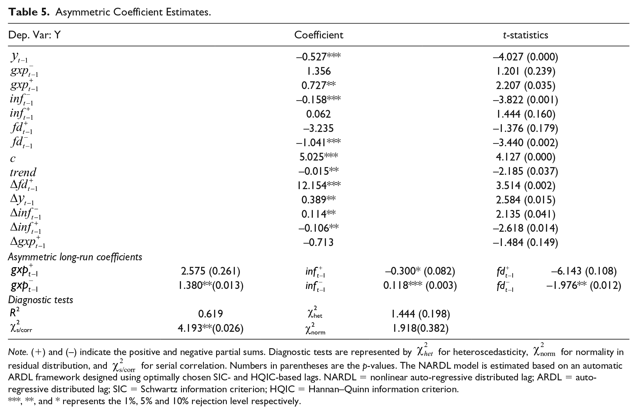
Note. (+) and (–) indicate the positive and negative partial sums. Diagnostic tests are represented by $χ_{h e t}^{2}$ for heteroscedasticity, $χ_{norm}^{2}$ for normality in residual distribution, and $χ_{s / corr}^{2}$ for serial correlation. Numbers in parentheses are the p-values. The NARDL model is estimated based on an automatic ARDL framework designed using optimally chosen SIC- and HQIC-based lags. NARDL = nonlinear auto-regressive distributed lag; ARDL = auto-regressive distributed lag; SIC = Schwartz information criterion; HQIC = Hannan–Quinn information criterion.

***

,**, and * represents the 1%, 5% and 10% rejection level respectively.

With inflation, unlike the insignificant positive partial sum, the negative partial sum squares of inflation are significant and still confirming the asymmetric impacts of inflation on economic growth (Ehigiamusoe et al., 2019). Hence, in the long run, positive and negative partial squares are –0.3 and 0.118, respectively, and all are significant. This means that increase in inflation reduces economic growth by 0.3%, whereas its decrease correspondingly increases economic growth by 0.12%. Inferentially, long-term instable inflation can severely induce long-term detrimental effects on economic growth via reduced productivity, unsustainable tax structures, increased long-run unemployment, and straining of government expenditures to offset unpalatable effects by such growth detractors. The estimates show that the impact on magnitude by positive inflation shocks is greatly detrimental compared with by negative inflation shocks, implying growth responds by a large slump to inflationary pressures. In the interactive environment, the trade-off implies that high and uncertain inflation that decreases financial returns implicatively deters investments and credit availability to demean financial developments, whereas the effects offset economic growth. In a similar case, results by Odhiambo (2009a) conversely posit that increasing inflation via spurring financial developments increases economic growth. This implies that high inflation is associated with employment opportunities, which increases income to households. With increased income and improved living standards, they save and invest more creating demand for financial services, intermediaries, and institutions whose development through technological and innovational inputs in turn causes real growth. The negative impacts of high inflation on real growth in this study support Hongo et al.’s (2019) results for Kenya and also concur with the results of Ehigiamusoe et al. (2019) on the panel of both high- and middle-income countries that inflation indirectly impacts growth via its negative externalities on financial deepening with inflation-stricken nations.

Exploring short-run results and starting with inflation, the significant positive and negative partial sum shocks by inflation have elasticities of −0.106 and 0.114, respectively. That is, short-run decrease in inflation increases economic growth by 0.114%, whereas its increase accordingly decreases growth by 0.12%. We notice that in the short run inflation trades off with economic growth, indicating lowering inflation remedies economic growth, whereas its increase is detrimental to growth. The growth inflation trade-off is ramified in studies of Hongo et al. (2019) in Kenya that decreasing inflation positively impacts economic growth and growth of financial institutions; however, the trade-off impact happens at a relatively lesser coefficient than in this study. More, because inflation infers to the long-run price uncertainties, the impact of long-run negative inflation shocks on growth in these works concurs with that of Fousekis et al. (2016) in the United States where uncertainties by inflation heighten retail and wholesale prices as general consumptive activities reduce and as general economic growth is affected. To round up, inflation through its negative and positive shocks poses confounding impacts on economic growth in Kenya in both the short and long run. The positive shocks devastate growth in the short run, whereas in the long run, increasing inflation to beyond unsustainable levels offsets economic activities while reducing general growth.

Financial development has also significant partial sum of squares and still demonstrates the importance of its asymmetric contributions to economic growth as in studies of Tsagkanos et al. (2019). Thus, in the long run, negative partial shocks are only significant with the coefficient at −1.976 and are noted to elastically decrease economic growth by 1.98%. However, in the short run, the significant positive partial sum of squares for financial development increases economic growth by 12.15%. These results concur with those of Nyasha and Odhiambo (2017) in Kenya, Jalil and Feridun (2011) in Pakistan, Calderón and Liu (2003) in 87 emerging countries, Adeniyi et al. (2015) in Nigeria, and Musila and Yiheyis (2015) in Kenya. Neo- classicist theory suggests that economic development and FDIs directly relate; this empirical finding ramifies that of Kinuthia and Murshed (2015) that increasing financial developments boost FDIs and thus economic growth. This implies that increased foreign investment influx brings with it new technologies, skills, and foreign capital while boosting economic activities and infrastructural developments, creating new job opportunities, and improving the living standards positively. With increased credit availability for investments as well as income to households for consumption and partly investments, economic activities are therefore heightened as positive growth happens.

The insignificant long-run positive shocks concur with Hermes and Lensink’s (2003), a postulation that positive effects of FDI cannot be attained with rigid financial and human developments and an implication that the complementary effects of financial development and FDIs positively support economic growth. In addition, their interactive environment has proved critical in increasing growth, and this is shown by Hermes and Lensink (2003) who interactively use FDIs with broad money/GDP and illustrate a positive impact on economic growth for 67-panel countries. Furthermore, this result confirms the significance of a relatively stable financial system which is important in attracting investments that induce capital formation and technological spillovers that positively fast tracks the ease with which capital is efficiently accumulated and utilized as technology is absorbed toward sustainable production.

On average and if financial development, inflation, and government expenditure are kept constant, the underlying rate of economic growth is at 5.03% and is slightly below the projected 5.6% to 8% in 2019. However, the growth rate trends negatively at 0.02%, which still demands for robust growth policies if the country’s envisioned “Big four” agenda (i.e., universal health care service, affordable housing, manufacturing, and food security) are to be achieved in the near future. Also, the short-run coefficient of GDP is significant. This means that current rates of economic growth are greatly predicted by previous information of economic growth which works to increase current growth at 0.39%. The end impact shows that previous growth information reduces growth by 0.58% rate, thus the need for sustainable real growth.

From the rear part of the table, diagnostic tests depict that 68% variations are comfortably explained by the ARDL (1,1,1,1) model, qualifying the model as best fitting. Also, the insignificant chi-square statistics by $χ_{het}^{2} (1.44)$ and $χ_{norm}^{2} (1.92)$ insinuates that the residuals have a constant variance and are normally distributed, respectively. However, the statistically significant serial correlation test statistic ( $χ_{s / corr}^{2} (4.19)$ ) denotes that the residuals might be suffering from autocorrelation, although the estimates are still unbiased and consistent.

In addition, stability tests executed by plotting the recursive CUSUM and CUSUMSQ statistics against the breakpoints and testing based on the null hypothesis that parameters are unstable are presented in Figures 1 and 2. This is the CUSUM and CUSUMSQ statistics stability test (Brown et al., 1975) plotted to ascertain the significance of trajectory at the 95% confidence bounds. In this faith, Figures 1 and 2 show rejection of null hypothesis. We therefore conclude that parameters in this regression are all stable

Figure 1.

Cumulative sum test of stability.

Figure 2.

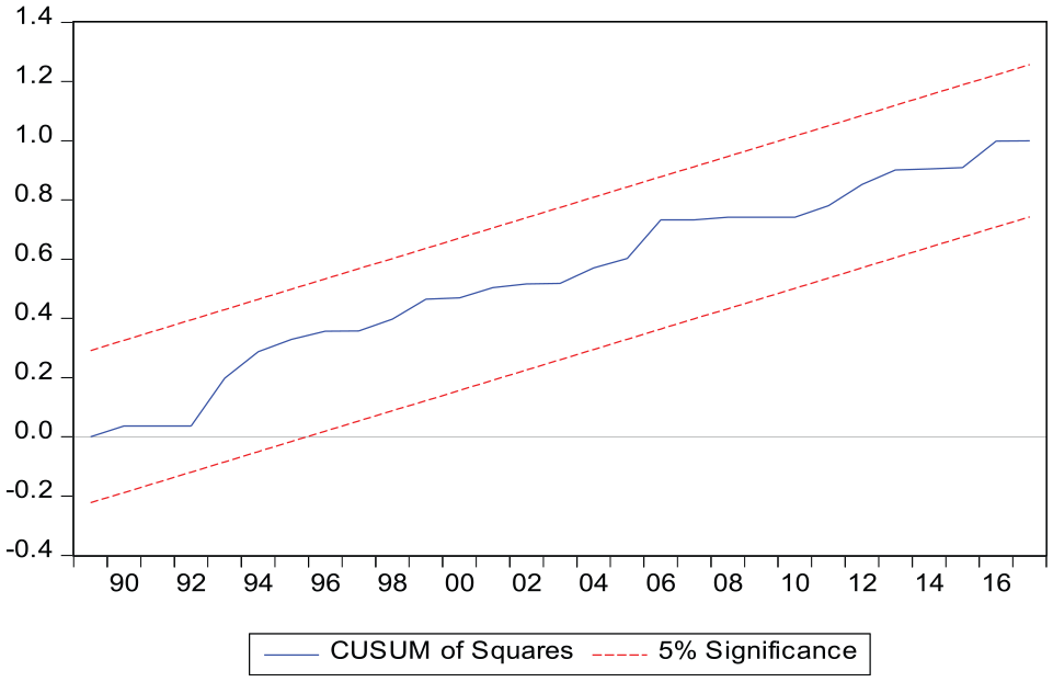
CUSUM sum of squares stability test.

We finally explore the dynamic multiplier to demonstrate the end temporal dynamics in growth while adjusting to a backdrop invented by both initial disequilibrium and short-run dynamics due to unprecedented shocks to financial development, expenditure and inflation. Rejection of the null by Table 3 supports existence of this initial equilibrium, and therefore, investigation of Figures 3 and 4 provides an insight into the validity of asymmetries presented in Table 5. Therefore, regarding Figure 3, positive financial shocks and negative government expenditure shocks are significant and most domineering. However, short-run dynamics are characterized by both shocks to growth except for government expenditure where negative shocks are thrilling growth, but in all cases, the disequilibrium is corrected roughly after six periods(years). In Figure 4, similar case is observed but with positive inflation shocks as most domineering.

Figure 3.

Dynamic multipliers.

Figure 4.

Dynamic multiplier; inflation on growth.

From the above, we infer that, first, growth responds gradually to an increase in financial development and decrease in government expenditure but with sharp boom to increasing inflation in the short run as long run is associated with correction. Second, the dynamics and disequilibrium are corrected approximately six periods ahead with response to new equilibrium achieving after a generally prolonged period. Third, the most important shocks are ones increasing financial development, decreasing government expenditures, and facilitating sustainable inflation. We conclude that specific policies that heighten financial system development, offset state expenditure but promote its prudent spending, and sustain appropriate inflation levels to the long run should be implemented.

In general, interesting results have been put forward regarding the effect of macroeconomic variables on growth. Sustainable inflation, increased financial developments, and reduced government expenditure responsibly will cause long-run economic growth and development. Inflation that boosts growth in the short run via short-run booming economic activities and increased productivity and creation of employment opportunities with increased welfare of citizens partly attracts financial system developments and prudent government expenditure to sustain productive growth in the long run. This calls for fiscal policy reforms which by reducing expenditure of public resources come along with other production-oriented policies such as efficient tax incentive structures, public administration efficacy, and prudency and accountability of public resources which offset rent-seeking behaviors and corruption to sustain in the long run; the growing economy supports financial structure integration. The supportive environment therefore creates need for productive financial reforms via heightening integration and development of financial systems and institutions, which in turn boosts the liberty, liquidity, and transparency of stock market developments. This backdrop also attracts foreign investors and investments that prefer integrated and stable financial systems, and with their inflowing technological skills and capital, their spillover effects further boost prospective financial development, which in turn creates employment opportunities and increased growth. The improved quality of financial systems in turn partially condenses some of the inflationary pressures due to improperly structured long-run monetary policies and continually leaving relatively high but sustainable inflation to increase economic growth. This argument is supported by the effects represented in Figures 3 and 4 that increase financial development but reduce government expenditure to offset the negativities by inflationary gap (high inflation) to positively cause growth. This is in consideration that economic growth sharply responds to high inflation with great slump than the ascend with financial development.

Conclusion

This article explored the asymmetric impacts of financial development, government expenditure, and inflation on economic growth in Kenya based on a nonlinear ARDL. The most critical results report that increasing financial development, reducing government expenditure. and sustainable inflation if implored would heighten long-term prospective goals and economic growth. The confirmation of the supply-led hypothesis implies that short-run financial reforms that attract sound financial development projects until the long run should be enhanced. Similarly, policies that support relatively increasing inflation in the short run to boosting booming economic activities but sustainable in the long run will be fruitful in growing the economy. As reduced government expenditure increases growth in the end, long-term policies that curb unnecessary government wastage but prudent public accountability and administration, and incarcerate rent dissipation and corruption proceeds should be put in place. Probably, what need to be reduced are the negativities of high government expenditure and inflation to growth as financial system integration should be heightened.

Since previous periods, the Kenyan government has implemented many economic development reforms touching the financial sector aside from the general infrastructural development and import shocks (like the oil crisis) which we believe have supplemented the temporal asymmetric behaviors in the financial development process and altered the stance of inflationary pressure toward growth. This implies a lot has happened in altering the stability of such macroeconomic structures and building a study point this article failed to explore. We therefore recommend reexamination of the herein studied impacts but in account of structural breaks.

Footnotes

Appendix

Table A1.

The Data Set Statistic.

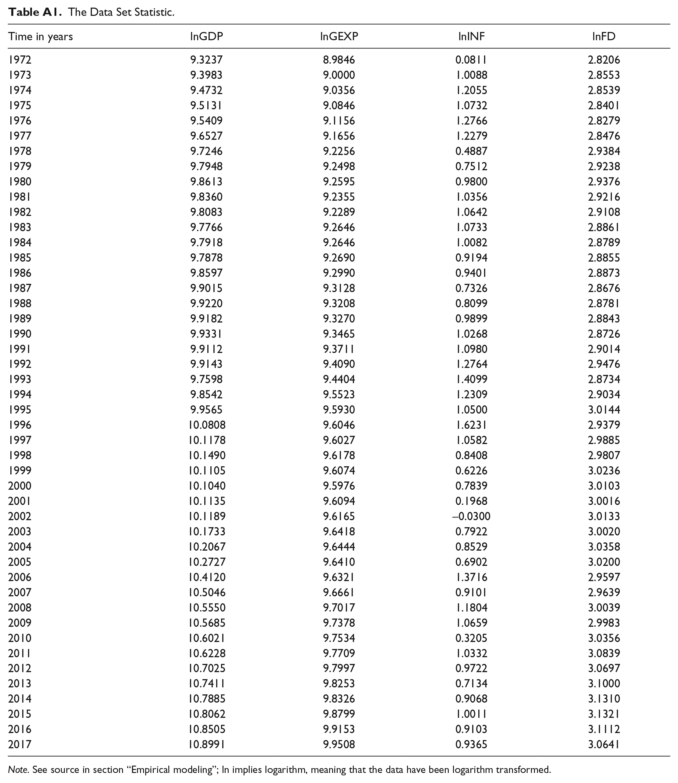
Time in years	lnGDP	lnGEXP	lnINF	lnFD
1972	9.3237	8.9846	0.0811	2.8206
1973	9.3983	9.0000	1.0088	2.8553
1974	9.4732	9.0356	1.2055	2.8539
1975	9.5131	9.0846	1.0732	2.8401
1976	9.5409	9.1156	1.2766	2.8279
1977	9.6527	9.1656	1.2279	2.8476
1978	9.7246	9.2256	0.4887	2.9384
1979	9.7948	9.2498	0.7512	2.9238
1980	9.8613	9.2595	0.9800	2.9376
1981	9.8360	9.2355	1.0356	2.9216
1982	9.8083	9.2289	1.0642	2.9108
1983	9.7766	9.2646	1.0733	2.8861
1984	9.7918	9.2646	1.0082	2.8789
1985	9.7878	9.2690	0.9194	2.8855
1986	9.8597	9.2990	0.9401	2.8873
1987	9.9015	9.3128	0.7326	2.8676
1988	9.9220	9.3208	0.8099	2.8781
1989	9.9182	9.3270	0.9899	2.8843
1990	9.9331	9.3465	1.0268	2.8726
1991	9.9112	9.3711	1.0980	2.9014
1992	9.9143	9.4090	1.2764	2.9476
1993	9.7598	9.4404	1.4099	2.8734
1994	9.8542	9.5523	1.2309	2.9034
1995	9.9565	9.5930	1.0500	3.0144
1996	10.0808	9.6046	1.6231	2.9379
1997	10.1178	9.6027	1.0582	2.9885
1998	10.1490	9.6178	0.8408	2.9807
1999	10.1105	9.6074	0.6226	3.0236
2000	10.1040	9.5976	0.7839	3.0103
2001	10.1135	9.6094	0.1968	3.0016
2002	10.1189	9.6165	−0.0300	3.0133
2003	10.1733	9.6418	0.7922	3.0020
2004	10.2067	9.6444	0.8529	3.0358
2005	10.2727	9.6410	0.6902	3.0200
2006	10.4120	9.6321	1.3716	2.9597
2007	10.5046	9.6661	0.9101	2.9639
2008	10.5550	9.7017	1.1804	3.0039
2009	10.5685	9.7378	1.0659	2.9983
2010	10.6021	9.7534	0.3205	3.0356
2011	10.6228	9.7709	1.0332	3.0839
2012	10.7025	9.7997	0.9722	3.0697
2013	10.7411	9.8253	0.7134	3.1000
2014	10.7885	9.8326	0.9068	3.1310
2015	10.8062	9.8799	1.0011	3.1321
2016	10.8505	9.9153	0.9103	3.1112
2017	10.8991	9.9508	0.9365	3.0641

Note. See source in section “Empirical modeling”; ln implies logarithm, meaning that the data have been logarithm transformed.

Authors’ Consent

The aforementioned authors had a unanimous consensus to all processes undertaken towards the paper.

Compliance With Ethical Standards

This paper complied with the ethical standards of the journal.

Declaration of Conflicting Interests

The author(s) declared no potential conflicts of interest with respect to the research, authorship, and/or publication of this article.

Funding

The author(s) disclosed receipt of the following financial support for the research, authorship, and/or publication of this article: Research was supported by Jiangsu Provincial Government Scholarship Program (190194) and National Social Science (18BGL255).

ORCID iD

Duncan O. Hongo

Notes

References

Abu-Bader

Abu-Qarn

. (2008a). Financial development and economic growth: Empirical evidence from six MENA countries. Review of Development Economics, 12(4), 803–817.

Abu-Bader

Abu-Qarn

. (2008b). Financial development and economic growth: The Egyptian experience. Journal of Policy Modeling 30, 887–898.

Adeniyi

Oyinlola

Omisakin

Egwaikhide

F. O.

(2015). Financial development and economic growth in Nigeria: Evidence from threshold modelling. Economic Analysis and Policy, 47, 11–21.

Anderson

Hunt

Snudden

(2014). Fiscal consolidation in the euro area: How much pain can structural reforms ease? Journal of Policy Modeling, 36(5), 785–799.

Atindehou

Gueyie

J. P.

Amenounve

E. K.

(2005). Financial intermediation and economic growth: Evidence from Western Africa. Applied Financial Economics, 15(11), 777–790.

Banerjee

Dolado

Mestre

(1998). Error-correction mechanism tests for cointegration in a single-eq9 framework. Journal of Time Series Analysis, 19(3), 267–283.

Batuo

Mlambo

Asongu

(2018). Linkages between financial development, financial instability, financial liberalisation and economic growth in Africa. Research in International Business and Finance, 45, 168–179.

Bencivenga

V. R.

Smith

B. D.

(1991). Financial intermediation and endogenous growth. The Review of Economic Studies, 58(2), 195–209.

Brown

R. L.

Durbin

Evans

J. M.

(1975). Techniques for testing the constancy of regression relationships over time. Journal of the Royal Statistical Society: Series B (Methodological), 37(2), 149–163.

10.

Calderón

Liu

(2003). The direction of causality between financial development and economic growth. Journal of Development Economics, 72(1), 321–334.

11.

Deltuvaitė

Sinevičienė

(2014). Investigation of relationship between financial and economic development in the EU countries. Procedia Economics and Finance, 14, 173–180.

12.

Demirgüç-Kunt

Levine

(1999). Bank-based and market-based financial systems: Cross-country comparisons. The World Bank.

13.

Dinh Thanh

Canh

N. P

. (2019). Dynamics between government spending and economic growth in China: an analysis of productivity growth. Journal of Chinese Economic and Business Studies, 17, 189–212.

14.

Dzhumashev

(2014). The two-way relationship between government spending and corruption and its effects on economic growth. Contemporary Economic Policy, 32(2), 403–419.

15.

Ehigiamusoe

K. U.

Guptan

Narayanan

(2019). The effects of income and inflation on financial development: Evidence from heterogeneous panels (Economics Discussion Papers No. 2019-11). Kiel Institute for the World Economy. http://www.economics-ejournal.org/economics/discussionpapers/2019-11/file

16.

Enders

(2015). Applied econometric time series. Wiley. (Original work published 2014)

17.

Fousekis

Katrakilidis

Trachanas

(2016). Vertical price transmission in the US beef sector: Evidence from the nonlinear ARDL model. Economic Modelling, 52, 499–506.

18.

Graff

(1999). Financial development and economic growth–A new empirical analysis (Dresden Discussion Papers in Economics No. 5/99). https://papers.ssrn.com/sol3/papers.cfm?abstract_id=258928

19.

Hermes

Lensink

(2003). Foreign direct investment, financial development and economic growth. The Journal of Development Studies, 40(1), 142–163.

20.

Hongo

O. D.

Ssali

M. W.

(2019). Trade-off Phillips curve, inflation and economic implication: The Kenyan case. International Journal of Economics and Finance, 11(4). http://www.ccsenet.org/journal/index.php/ijef/article/view/0/38858

21.

Jalil

Feridun

(2011). Impact of financial development on economic growth: Empirical evidence from Pakistan. Journal of the Asia Pacific Economy, 16(1), 71–80.

22.

Kar

Nazlıoğlu

Ş.

Ağır

(2011). Financial development and economic growth nexus in the MENA countries: Bootstrap panel granger causality analysis. Economic Modelling, 28(1–2), 685–693.

23.

Kariuki

P. W.

(1995). The impact of interest rate liberalisation on financial savings: The case of Kenya. African Review of Money Finance and Banking, 9, 5–23.

24.

Katrakilidis

Trachanas

(2012). What drives housing price dynamics in Greece: New evidence from asymmetric ARDL cointegration. Economic Modelling, 29(4), 1064–1069.

25.

Khemili

Belloumi

(2018). Cointegration relationship between growth, inequality and poverty in Tunisia. International Journal of Applied Economics, Finance and Accounting, 2(1), 8–18.

26.

Kinuthia

Murshed

(2015). FDI determinants: Kenya and Malaysia compared. Journal of Policy Modeling, 37, 388–400.

27.

Klobodu

E. K.

Adams

M. S.

(2016). Capital flows and economic growth in Ghana. Journal of African Business, 17(3), 291–307.

28.

Lawrence

I. A.

Osedebamhen

Eikhomun

D. E.

(2014). Development of financial system and economic growth: An empirical evidence from Nigeria. European Journal of Business and Management, 6(30), 137–152.

29.

Levine

(1997). Financial development and economic growth: Views and agenda. Journal of Economic Literature, 35(2), 688–726.

30.

Levine

Loayza

Beck

(2000). Financial intermediation and growth: Causality and causes. Journal of Monetary Economics, 46(1), 31–77.

31.

Lucas

R. E.

(1988). On the mechanics of economic development. Journal of Monetary Economics, 22(1), 3–42.

32.

Musila

J. W.

Yiheyis

(2015). The impact of trade openness on growth: The case of Kenya. Journal of Policy Modeling, 37(2), 342–354.

33.

Narayan

P. K.

Narayan

(2013). The short-run relationship between the financial system and economic growth: New evidence from regional panels. International Review of Financial Analysis, 29, 70–78.

34.

Nawaz

Lahiani

Roubaud

(2019). Natural resources as blessings and finance-growth nexus: A bootstrap ARDL approach in an emerging economy. Resources Policy, 60, 277–287.

35.

Nyaranga

M. S.

Hao

Hongo

D. O.

(2019). Strategies of integrating public participation in governance for sustainable development in Kenya. Public Policy and Administration Research, 9(7). https://www.iiste.org/Journals/index.php/PPAR/article/view/48764/50602

36.

Nyasha

Odhiambo

N. M.

(2017). Banks, stock market development and economic growth in Kenya: An empirical investigation. Journal of African Business, 18(1), 1–23.

37.

Odhiambo

N. M.

(2009a). Finance-growth nexus and inflation dynamics in Kenya: An empirical investigation. Savings and Development, 33(1), 7–25.

38.

Odhiambo

N. M.

(2009b). Interest rate reforms, financial deepening and economic growth in Kenya: An empirical investigation. The Journal of Developing Areas, 43, 295–313.

39.

Patrick

H. T.

(1966). Financial development and economic growth in underdeveloped countries. Economic Development and Cultural Change, 14(2), 174–189.

40.

Pesaran

M. H.

Sin

Smith

R. J.

(2001). Bounds testing approaches to the analysis of level relationships. Journal of Applied Econometrics, 16(3), 289–326.

41.

Rousseau

P. L.

Vuthipadadorn

(2005). Finance, investment, and growth: Time series evidence from 10 Asian economies. Journal of Macroeconomics, 27(1), 87–106.

42.

Saci

Holden

(2008). Evidence on growth and financial development using principal components. Applied Financial Economics, 18(19), 1549–1560.

43.

Schumpeter

J. A.

(1911). The theory of economic development: An inquiry into profits, capital, credit, interest and the business cycle ( Opie

Redvers

, Trans. 2008 ed.). Transaction Publishers.

44.

Shin

Greenwood-Nimmo

(2014). Modelling asymmetric cointegration and dynamic multipliers in a nonlinear ARDL framework. In Sickles

R. C.

Horrace

W. C.

(Eds.), Festschrift in honor of Peter Schmid (pp. 281–314). Springer.

45.

Sobiech

(2019). Remittances, finance and growth: Does financial development foster the impact of remittances on economic growth? World Development, 113, 44–59.

46.

Solow

R. M.

(1960). Investment and technical progress. Mathematical Methods in the Social Sciences, 1, 48–93.

47.

Tsagkanos

Siriopoulos

(2015). Stock markets and industrial production in north and south of Euro-zone: Asymmetric effects via threshold cointegration approach. The Journal of Economic Asymmetries, 12, 162–172.

48.

Tsagkanos

Siriopoulos

Vartholomatou

(2019). Foreign direct investment and stock market development: Evidence from a new emerging market. Journal of Economic Studies, 46(1), 55–70.

49.

Ujunwa

Pius

S. O.

(2010). Stock market development and economic growth: Evidence from Nigeria. European Journal of Economics, Finance and Administrative Sciences, 25, 44–53.

The Asymmetric Influence of Financial Development on Economic Growth in Kenya: Evidence From NARDL

Abstract

Keywords

Introduction

Literature Review

Empirical modeling

Data

Methodology

Empirical Results and Analysis

Conclusion

Footnotes

Appendix

Authors’ Consent

Compliance With Ethical Standards

Declaration of Conflicting Interests

Funding

ORCID iD

Notes

References