Sage Journals: Discover world-class research

Abstract

This article presents an explanation to the paradox of why increased household incomes in rural areas in China are accompanied by decreased motivation for consumption. The empirical analysis shows a reduction in rural residents’ consumer spending with the exception of spending on medical treatment and education. This effect is stronger in poor families or families with school-aged children. The authors argue that motivation for consumption has been sinking in rural areas in China because income inequality among the rural populations has stimulated spending on improving human capital to promote individual security and social mobility as a chance to squeeze into the middle class.

Keywords

consumer motivation rural medical care rural education social mobility individual security

Introduction

Economic fluctuation and the changes in consumption structure of rural residents are two important aspects in the development of rural economy. Earlier economic studies show that when the household income increases, the ratios of consumption expenditure on food and clothing are with a downward trend, whereas other living expenses and nonliving expenses rise. This is usually termed the extension under Engel’s law. The index depicting this behavior is named as the “consumption intention index” in China. According to data of the National Bureau of Statistics survey in 2016,¹ Chinese residents’ consumption willingness dropped from 82% in 1997 to 75% in 2006, and dropped to a low 15% in 2016. The American scholars who have studied this suggest that the main factors affecting the social consumption tendency are that the relationship between income and labor is becoming more relaxed, families are smaller, the tertiary industry is prosperous, social service are improving, and social security is enhanced (Cowell, 1989; Kraay, 2000; Kuijs, 2006; Wen, 2016). However, these phenomena are just partially occurring in China’s rural areas. Consumption costs spent for food account for a major proportion of the entire consumer expenditures and the income growth is still the key factor that influences the consumption in rural China (Zhou & Wang, 2011). In addition to income, social welfare becomes the important factor affecting rural residents’ consumption (Zhang & Zhao, 2017). While the reduced proportion of consumer consumption in the rural areas of China is much higher than that of the urban residents, the income growth of rural residents is far more than the urban residents. This produces a paradox.

The authors are satisfied that the reason a smaller income increase since 1999 constrains consumption motivation to a larger extent in rural areas than urban areas is because of a greater lack of a sense of security with regard to residents’ medical care and access to considerable education in the rural areas. The cause of the lopsided proportion of consumption expenditure in the rural areas is generated by a need for security and the desire for increased social mobility. Even with a slight increase in income, and the chance of the rural population to leave the vicious spiral of low-income poverty, their income will have a return that is proportional to an increase in social status. The returns they desire with higher income include a sense of well-being. Therefore, the rural residents, in the pursuit of well-being and social mobility, will continue to increase investment spending in health and education so as to be able to squeeze into a higher social class.² The empirical results also show the fact that the proportion of education and medical cost on consumption expenditures are gradually increased, which also limited the expansion of consumption (Fang & Wang, 2011; Xu & Li, 2015; Yuan & Xia, 2017).

The income gap between rural residents, however, shows an upward trend since China’s reform and opening up period started 30 years ago, from 0.403 in 1981 to 0.520 in 2016.³ The Gini coefficient of the same type rural households’ in the same area rose from 0.4387 to 0.52001, 2006 to 2016. While the actual consumption was reduced by 4.2%, the consumption propensity fell 2.35%, during this period, and 28% of it can be explained by the income gap.⁴ To some extent, this can verify our assumption. Relative to high-income rural families, the low-income families will have a higher pursuit of well-being and the desire for social mobility.⁵ In this article, we focus on the analysis of the income gap and analyze how this affects the expenditures of family health and education.⁶ Other factors are also considered.

The article is divided into several parts: the first part is the introduction and literature review; the second part is further analysis of the literature and the presentations of the hypothesis; in the third part of the article, we will suggest a theoretical model; in the fourth part, we will introduce data and validate the proposed theoretical model by empirical comparisons; in the fifth part, we discuss the results of the Hausman test of the strength of the results of the empirical analysis. The last part of the article presents the conclusion and offers some suggestions for further research.

Education Pursuit, Health Demand, and Motivation

According to Abraham Maslow’s Theory of Hierarchy of Needs, the lowest level is the physiological needs. After basic needs of survival (water, air, food, and sleep), Maslow moves on to needs of security that are also important to survival. Security needs then move to social needs such as belonging and affection. According to Maslow, social needs are less basic than physiological and security need. In this article, we focus on the next level of needs defined by Maslow as “Esteem Needs.” We use the currently accepted term of “well-being.” Maslow means that esteem needs are needs that reflect on self-esteem, personal worth, social recognitions, and accomplishment. This category includes the need for obtaining a higher social status. It is possible to talk about a hierarchy of social mobility where individuals are motivated to obtain a higher social status. Weber (1922) suggested that individuals who see themselves as members of a higher social class will take all kinds of measures to control the accession of new members to maintain and build the authority and image of their own high social status. If this is in fact true, it is necessary to look at how social positions are established. Weiss and Fershtman (1998) believed that a particular social status was dependent on birth into a family position in society. Thus, each person’s social status was determined by the family wealth, education, occupation, and family background. This then introduces the idea of social class mobility. Does one move from a family with particular class identification to another? How much social mobility is there within a country and what makes it possible to embark on a “class trip,” either to a higher or lower position than the social position in which one was born? It is difficult to measure social mobility either intergenerational social mobility or introgenerational mobility where a person moves from one social class to another during the course of their lifetime. This article does not attempt to answer such questions of social mobility. Instead, we are using the idea of social mobility to a higher social status, or fear of declining to a lower social status, as a framework to understand changing consumption patterns.

Sociologically, we talk about two types of status. Ascribed states cannot be changed; they are inherited by virtue of family class, gender, and ethnic group. Achieved states are earned by individual effort.

There are different theoretical ways of explaining social mobility. A functionalistic theory would say that societies with a high degree or meritocratic access present many opportunities for social mobility and inequality and are the result of differences in effort and intelligence (Saunders, 2017). According to a neo-Marxist–oriented theory, social mobility does not exist but class society is reproduced and we stay in either a bourgeois or proletariat class. The third theory and one that will be explored further in this article is the “rational action theory.” This can be found in the work of John Goldthorpe (2007) who argues that people are “rational actors” who calculate relative costs and benefits of social mobility.⁷

The Gini coefficient in China’s rural area, as we pointed out, is constantly increasing. At the same time, the expenditures of medical and education have increased because of the factors such as economic development and inflation. This means, if we use Maslow’s hierarchy of needs as motivational to behavior, certain basic needs such as security and good health are not equally available to individuals (Qiang, 1997, 2002; Ye, Hongbin, & Binzhen, 2017). Due to the increase in costs for health care and the limitation of the New Cooperative Medical Schemes (NCMS), the rural residents face greater financial risks of disease and they lack a sense of security in the short-term future. Meanwhile, China has a tradition of dealing with unknown risks through saving, against this backdrop; people will suppress their consumption expenditures based on the need of security in the short-term future. Using Goldthorpe’s theory of rational action, for the rural resident, a higher social status can be a solution to material problems. Gaining access to a higher social class for a rural Chinese resident is usually seen as possible through the use of the educational system. Obtaining a higher education not only increases the chances for better positions in a country that is introducing meritocracy and achieved status, but also is beneficial for creating new networks and connections outside of more limited family relationships. Social mobility to a higher social class also influences access to more privileges and more access to distributional rights (Weiss & Fershtman, 1998).

Thus, as a rational actor, rural individuals can be seen as suppressing consumption patterns to use the majority of income for education investment and unknown financial risks of diseases. How do we know what factors will, in fact, increase social status? Research about this is not very extensive. Corneo & Jeanne (1998) mean that it is primarily wealth that influences social mobility.⁸ Needless to say wealth is a decisive factor, but education, health condition, and household registration can also affect the promotion of the social status for rural Chinese. However, if rural residents want to achieve better health care, higher education, and more comprehensive social security, the base factor is still increasing wealth. The research of Li Chunling (2005) and Ye, Hongbin, & Binzhen (2017) also showed that differences in social class and the creation of social stratification are dependent on differences of economic status.⁹ Thus, we will use the Gini coefficient as an indicator of social stratification and propose a series of problems in the article and discuss some conclusions.

First, we hypothesize that the income distribution of rural residents will affect the consumption structure. An increase in the Gini coefficients will restrain the consumption expenditure of rural households dynamically. Reduction in consumption will allow for a redistribution of income in a manner that will allow rural residents to squeeze into a higher social class by temporarily reducing consumption in favor of accumulating wealth.¹⁰ Second, as health is the most basic capability for humans to survival and development, and education is the most important way of human capital investment, rural residents will make the consumer motivation maximization in health and education spending to enter a higher social class. Finally, the influence of accumulation of wealth and constraints on consumer spending will have a greater effect on the population of low-income rural residents than the population of rural residents with higher incomes. The desire of improving social status among the older residents is far less than the younger, and motivation of the younger for cutting consumption expenditures except for investments in health care and education spending will be stronger.¹¹

Model Specifications

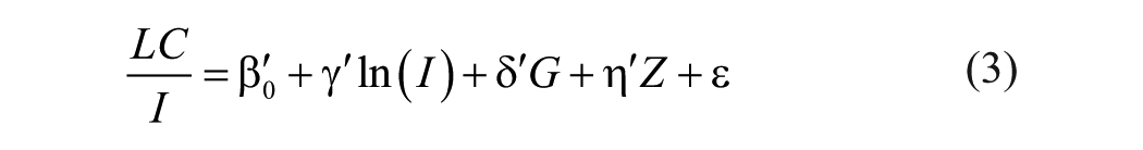
To verify the conclusions and assumptions, we will establish the model as follows:

\ln (L C) = β_{0} + γ \ln (I) + δ G + η Z + μ

(1)

where LC = family living costs excluding health and education spending,

I = disposable income of residents, G = Gini coefficient of rural residents,¹² Z = control variable.

We then can obtain the following model:

\ln (\frac{L C}{I}) = β_{0} + (γ - 1) \ln (I) + δ G + η Z + μ

(2)

where $L C / I$ = average propensity to consumption.

We find the variation of average propensity to consumption (APC) and the transformation of Equation 2:

\frac{L C}{I} = {β^{'}}_{0} + γ^{'} \ln (I) + δ^{'} G + η^{'} Z + ε

(3)

We take the provinces and cities where the rural households live and the rural residents in different age groups as the reference groups.¹³ In addition to the average difference of Gini coefficient, we also introduce the ratio of income between the highest income families and the lowest income households as an inequality index to measure the differences between the two extremes. At the same time, we estimate scale economy of rural families.¹⁴ Consumption expenditures of rural residents in different regions together with variation in aging patterns will produce differences in different years. To control for these changes, we introduce control mechanisms. The model’s estimation test can be processed through the income gap between different interval groups in the year to complete the progressive difference for the same area of the income difference and average income within the group due to correlation bias.¹⁵ Therefore, if we ignore the average income and do not control, we will undervalue the influence of Gini coefficient. We will estimate the difference of family living costs between the upper and lower classes which is caused by the income gap as follows:¹⁶

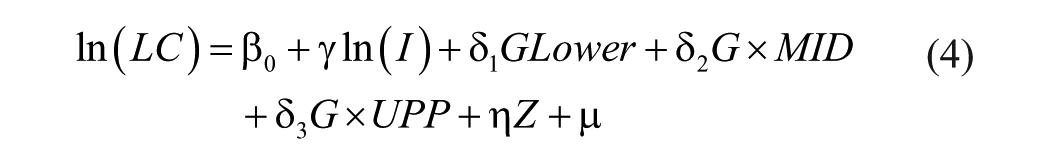
\begin{array}{l} \ln (L C) = β_{0} + γ \ln (I) + δ_{1} G L o w e r + δ_{2} G \times M I D \\ + δ_{3} G \times U P P + η Z + μ \end{array}

(4)

where Lower = lower income class, MID = middle class, UPP = the highest income class, δ₁ = influence on the income gap for lower class residents, δ₂ = influence on the income gap for middle class residents, δ₃ = influence on the income gap on upper class residents.¹⁷

Data and Empirical Results

We perform an empirical analysis by using the data from the National Bureau of Statistics taken from China’s rural household survey of 11 provinces or autonomous regions for the years 2006 to 2010, and we also use the relevant data for rural areas in China’s four major economic regions to perform an Hausman (1978) test analysis. The main data include rural households in five equal groups, three economic zones, and four regional economic groups. The basic data are about family members of rural residents. In order not to lose the representativeness, we select the rural areas data in four major economic regions to perform the empirical analysis. We use the income of the family as a unit because of the head of household generally decides patterns of consumer spending in rural China. To verify the hypotheses proposed, we choose related indexes that describe the primary worker in the family.¹⁸

The specific trend is shown in Figure 1.

Figure 1.

Change in APC and the Gini coefficient in China rural areas, 2006 to 2016.

We can see the changes in APC for rural households and the changes in Gini coefficient over 11 years.¹⁹ As shown in Figure 1, both APC (Average Propensity to Compensation) and APC_EME (Average Propensity to Compensation with the exception of medical care and education) are gradual declining from 2006 to 2016. Meanwhile, the interval between the curve of APC and the curve of APC_EME is similar, indicating that the proportion of education and medical care costs on overall consumption expenditures are stable during this period. Although the costs that people spent on educational services provided by the Chinese government are reduced during this period, in that the government exempted the tuition and miscellaneous fees for students in compulsory education since 2006 and the national financial expenditures on other types of schools also increased rapidly, they spend more on education services that are provided by the private education institutions. The medical care costs also increased with the development of medical technologies and inflation; at the same time, the role of NCMS is limited and the rural residents still spend more on medical care. As a result, the proportion of education and medical care costs on total consumption expenditures are stable during this period. The increase in the Gini coefficient, whether it is measured as between groups or within groups, has been accelerating for the entire period, 2006 to 2016.

In Figure 2, we can see that the inequality index shows increase–decrease–increase tendency with rising age of the rural resident.

Figure 2.

Change in APC and the Gini coefficient in China rural areas for different age groups, 2006 to 2016.

The income gap between rural residents reaches its peak at the age of 45. We also see from changes in the Gini coefficients that the gap measuring inequality for different age groups of rural residents is largest between 30 and 50 years old.

From the specific numerical values, we can see that the change in standard deviation is obvious, and the intragroup Gini coefficients’ difference is substantial. We use the ordinary least squares (OLS) method to analyze the changes of inequality and discuss the robustness of results. First of all, we will look at the decisions of family consumption motivation that are related to the pursuit of security and social status. Results of the regression are shown in Table 1.

Table 1.

Effect of the Income Gap on Rural Resident’s Family Consumption Decisions.

Independent variables	Dependent variable: Consumer spending
Independent variables	Model 1	Model 2	Model 3	Model 4
Gini coefficient	−0.466*** (0.076)	−0.453*** (0.076)	−0.405** (0.0763)	−0.507*** (0.213)
Disposable income	0.728** (0.002)	0.709*** (0.004)	0.711*** (0.006)	0.767** (0.014)
Five equal groups of income		▲	▲
Disposable Income × Five Equal Groups of Income			▲
Linear trend				▲
Observations	34,662	34,662	34,662	34,662
Adjusted R²	.761	.761	.761	.761

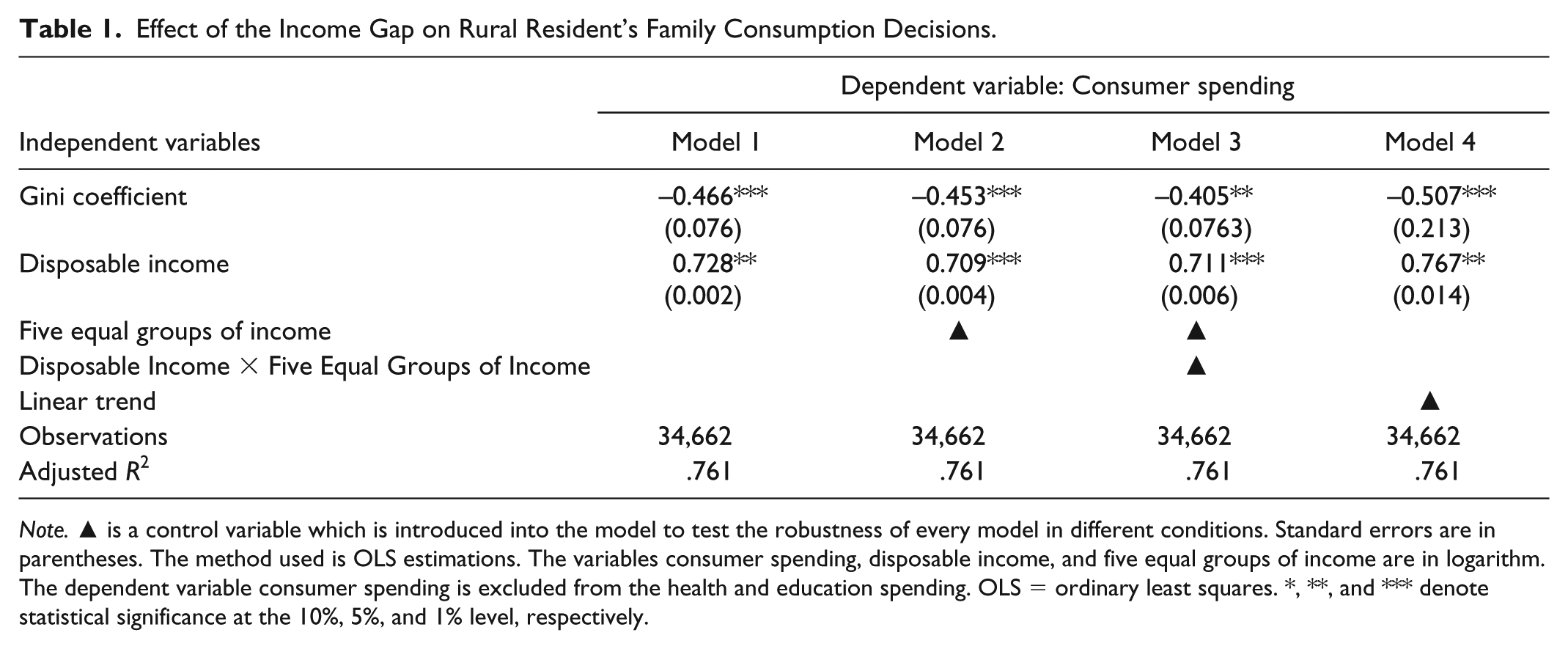
Note. ▲ is a control variable which is introduced into the model to test the robustness of every model in different conditions. Standard errors are in parentheses. The method used is OLS estimations. The variables consumer spending, disposable income, and five equal groups of income are in logarithm. The dependent variable consumer spending is excluded from the health and education spending. OLS = ordinary least squares. *, **, and *** denote statistical significance at the 10%, 5%, and 1% level, respectively.

From Table 1 we see that if we control for the variable rural household disposable income, the income gap still has significant influence on consumer spending, and the influence effect is negative. If the Gini coefficient increases by 1%, consumption will decline by 0.38%, which is the change in average consumption of rural residents. However, different residents have different consumption motivation and consumption tendency, and the consumption structure is not completely controlled by use of disposable income.²⁰

The results of income difference between rural residents affect the APC of families and show that the income gap between families has significantly negative effects on the APC. Model 1 shows (the other models are similar) that if there is a 1% increase in the Gini coefficient, then the APC will be reduced by 0.27%. Models 2 through 4 are robust. Therefore, results in Table 1 verify the hypothesis that the income gap between rural households can significantly constrain consumer motivation.

Next, we will analyze whether the different income gap influences consumption of the rural households with differing incomes. The resident households will be divided into three classes by status denoted on the basis of income. The analysis results are shown in Table 2.

Table 2.

Effect of Rural Inequality on the Consumption Patterns of Stratified Rural Families.

Independent variables	Dependent variable: Consumer spending
Independent variables	Model 1 (T)	Model 2 (L)	Model 3 (M)	Model 4 (U)
Gini coefficient	−0.614** (0.122)	−0.472*** (0.204)	−0.406*** (0.129)	−0.356** (0.207)
Disposable income	0.724** (0.004)	0.763*** (0.007)	0.827** (0.021)	0.760*** (0.024)
Gini Coefficient × Middle-Income Class	0.205*** (0.076)
Gini Coefficient × Upper Income Class	0.311** (0.083)
Observation	34,662	28,764	29,684	30,257
Adjusted R²	.72	.70	.68	.68

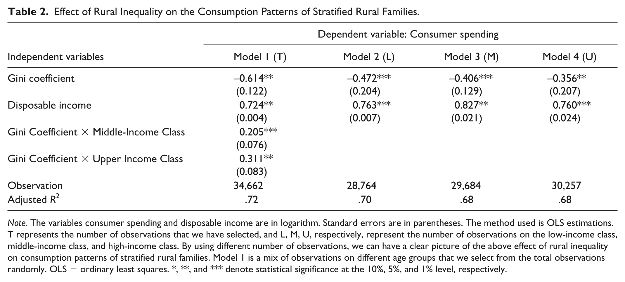
Note. The variables consumer spending and disposable income are in logarithm. Standard errors are in parentheses. The method used is OLS estimations. T represents the number of observations that we have selected, and L, M, U, respectively, represent the number of observations on the low-income class, middle-income class, and high-income class. By using different number of observations, we can have a clear picture of the above effect of rural inequality on consumption patterns of stratified rural families. Model 1 is a mix of observations on different age groups that we select from the total observations randomly. OLS = ordinary least squares. *, **, and *** denote statistical significance at the 10%, 5%, and 1% level, respectively.

From Model 1 in Table 2 we can see that the interaction term of variables income groups and the Gini coefficients passes the test, and it has a negative relationship with income. If the Gini coefficient increases by 1%, the consumption of low-income groups declines by more than 0.25% in comparison with the middle class of rural residents and more than 0.311% in comparison with the high-income groups. The results of Models 2 to 4 show that the inequality index measured by the Gini coefficient has a strong constraining effect on consumption of rural residents in the lower income class, and the constraining effect on residents in the high-income class is significantly weaker.

Because of the “cluster effect of income,” the richer group of rural residents shares more resources and has a wider range of wealth than the poor, and the wealth has an acceleration effect much like a “snowball” effect. However, the low-income group has finite resources, and the way to get wealth is narrow. If the low-income social stratum desires social mobility, they would have to have more wealth than the higher income group. In this sense, the possibility of low-income rural residents entering the high-income class is minimal. Eventually, we can assume that residents in the lower income group will lose the motivation for obtaining social mobility, and then they will increase consumption expenditure. But the empirical results show the contrary. When the Gini coefficient expands further, the low-income group of rural residents has much weaker consumer motivation than the higher income group. We proposed that the main reason is that people pursue not only material consumption but also a satisfaction of higher needs of esteem.²¹ They see a possibility for entering into the social middle class through higher education and from there the possibility of further improving their own social status through the accumulation of wealth.

Table 3 shows the effect of income gap within rural residents on household consumption decisions in different age groups. We can see that the younger the householder’s age, the larger is the influence of the Gini coefficient, which also is significant. We take the age interval group of 16 to 30 as the reference to analyze the consumption status of the other four groups. The effect of increased inequality on the consumption motivation shows a downward trend with increasing age. However, the age interval group of 56 to 60 and 61 to 105 is a jumping point, whereas after the age of 60, the effect of inequality rapidly disappears.

Table 3.

Effect of Inequality on Consumption Decisions for Different Age Groups.

Independent variables	Dependent variable: Consumer spending
Independent variables	Model 1 (T)	Model 2 (Y)	Model 3 (O)	Model 4 (T)
Gini coefficient	−0.304*** (0.125)	−0.629*** (0.117)	−0.275(0.206)	−0.583** (0.230)
Disposable income	0.819*** (0.005)	0.810*** (0.003)	0.824** (0.006)	0.875** (0.002)
Age of (16-30) × Gini Coefficient	−0.208*** (0.217)
Age of (16-30) × Gini Coefficient				0.355(0.130)
Age of (30-55) × Gini Coefficient				0.347(0.211)
Age of (55-60) × Gini Coefficient				0.167(0.212)
Age of (60-105) × Gini Coefficient				0.684** (0.191)
Observations	34,662	37,814	30,881	34,662
Adjusted R²	.72	.78	.70	.72

Note. The variables consumer spending and disposable income are in logarithm. Standard errors are in parentheses. The method used is OLS estimations. By controlling the interaction term Age of (16-30) and Gini Coefficient, we can obtain Model 1; we can also obtain Model 4 by controlling the interaction terms in Table 3 excluding the interaction term Age of (16-30) and Gini Coefficient. T is the number of observations; Y is the number of observations on the young (16-30); O is the number of observations on the old (60-105). OLS = ordinary least squares. *, **, and *** denote statistical significance at the 10%, 5%, and 1% level, respectively.

From Table 4 we see that the differences on the expenditure of medical care and the human capital investment between the low-income and high-income groups are not significant. From Models 3 to 6, we can see that when the Gini coefficient increases, the growth ratio of the education investment in low-income families is higher than the middle- and high-income families. Only by investing in human capital, the low-income families can gain access to a higher social class.

Table 4.

Effect of Rural Inequality on Expenditure for Education and Medical Care.

Independent variables	Expenditure for education and medical care
Independent variables	Model 1	Model 2	Model 3 (L)	Model 4 (M)	Model 5 (U)	Model 6
Gini coefficient	5.830*** (0.438)	4.067** (0.986)	2.835(1.659)	2.467** (1.519)	2.528(1.386)	−3.261*** (2.037)
Disposable income	0.806** (0.427)	0.667** (0.461)	0.799** (0.071)	0.495** (0.206)	0.822** (0.073)	0.792*** (0.047)
Middle-Income Class × Gini Coefficient		0.626(0.102)
Upper Income Class × Gini Coefficient		−0.796(0.120)
Age of (16-30) × Gini Coefficient						7.394** (1.590)
Observations	34,662	34,662	15,461	15,264	12,543	30,246
Adjusted R²	.19	.19	.16	.18.	.20	.15

Note. The variables expenditure for education and medical care, disposable income are in logarithm. Standard errors are in parentheses. The method used is OLS estimations. L, M, and U, respectively, represent the number of observations on the low-income class, middle-income class and high-income class. The difference between Models 1 and 2 is that we have used different control variables. For Model 6, we have used different number of observations and control variables comparing Models 1 and 2. OLS = ordinary least squares. *, **, and *** denote statistical significance at the 10%, 5%, and 1% level, respectively.

Robustness Test

An increase in the Gini coefficient will lead to a constraint of consumption with the exception of spending on health and education among the low-income groups. This is interpreted as motivated by investing in human capital to improve their social status. However, the cost of the basic necessities of life cannot be compressed infinitely; the above empirical results of the constraining effect on consumption of increased inequality present a paradox. To further examine restraints on consumption with the exception of consumption for health and education, we then refine the cost of living expenses, and we use the expenditure for food and clothing to measure the cost of living expenditure. The test results are shown in Table 5.

Table 5.

Hausman Test for Testing Endogeneity of Food Expenditure, Clothing, and Consumption Patterns.

Dependent variable	Food expenditure	Clothing expenditure	Consumer spending	Consumer spending
Dependent variable	Model 1	Model 2	Model 3	Model 4
Gini coefficient	−0.525*** (0.213)	−0.298(0.219)	−0.451(0.003)	−0.528*** (0.212)
Disposable income	0.851*** (0.003)	0.807*** (0.003)	0.852*** (0.003)	0.827*** (0.00)
Floor space				0.068(0.051)
Weighting of (16-30)				−0.029(0.002)
Transfer income				−0.235*** (0.048)
Expectations of future income	0.063(0.063)	−0.086** (0.061)		−0.522*** (0.067)
Relief rate of minimum living security system			0.356*** (0.030)	0.354*** (0.031)
Rate of sharing new rural endowment insurance			0.205*** (0.024)	0.210** (0.027)
Observation	7,655	7,768	8,562	7,358
Adjusted R²	.72	.73	.75	.79

Note. The variables expenditure for food, clothing, disposable income transfer income, floor space, and expectations of future income are in logarithm. Standard errors are in parentheses. The method used is OLS estimations. OLS = ordinary least squares. *, **, and *** denote statistical significance at the 10%, 5%, and 1% level, respectively.

The results of the Hausman test on the clothing expenditure and consumption expenditure of Models 2 and 3 are not significant. However, when adding more indexes which reflect the cost of living, the impact of the Gini coefficient on the rural residents’ living consumption becomes significant (as in Model 4).

The empirical results show that raising the Gini coefficients will compress the rural residents’ living expenses in addition to spending on health and education, and the empirical results also show that the reason for this phenomenon is that rural residents pursue avenues leading toward social security and social mobility. However, we would want to know whether or not there are other factors determining consumption such as uncertain future income.²² We combine it with the actual situation of Chinese rural residents and discard this possibility.²³ The results of empirical analysis show that the correlation between rural households’ income gap and the expenditure of living consumption is not due to the uncertainty of future income.

In addition, the rising Gini coefficient may have negative effect on low-income rural residents’ old-age security. It could contribute to a behavior of “saving for the future” according to a life cycle theory. However, there are two scientifically diametrically opposed views to this problem (see, for example, the supporting “saving for the future” (Martin, 1974), as opposed to the argument of constraints on saving behavior (Kotlikoff, 1981)). In fact, there is no conclusion that the social security system has constraining or facilitating effects on consumption, and this, in turn, depends on the sizes of the two effects. It is difficult to determine the magnitude of effect. And we may identify the results as significant but only temporarily. In Table 5, Model 4 includes all relevant variables. The results show that a number of possible variables have no effect on consumption patterns. In addition to the Hausman test on endogeneity, we also test the upper and lower limits of variation in consumption.²⁴

The results in Table 6 show that the unexplained residuals of the Gini coefficient have little difference from the overall distribution of the tested variables. When the value of upper income/lower income increases by 1%, the consumption expenditure of rural residents will fall by 0.1036%. The constraining effect of increased inequality on consumption is much higher for the low-income class than that of the high-income class.

Table 6.

Hausman Test on the Variable Upper Income/Lower Income.

Dependent variable	Food expenditure	Clothing expenditure	Living expenditure	Living expenditure
Dependent variable	Model 1	Model 2	Model 3	Model 4
Upper income/lower income	−0.045*** (0.009)	−0.071** (0.021)	−0.019** (0.024)	0.308*** (0.221)
Disposable income	0.755*** (0.004)	0.791*** (0.004)	0.757** (0.004)	0.894*** (0.031)
Proportion of 3/5 income households		0.042*** (0.024)
Proportion of 5/5 income households		0.047*** (0.022)
Weighting of (16-30)			−0.021*** (0.023)
Observations	13,214	13,214	13,214	9,875
Adjusted R²	.71	.75	.72	.23

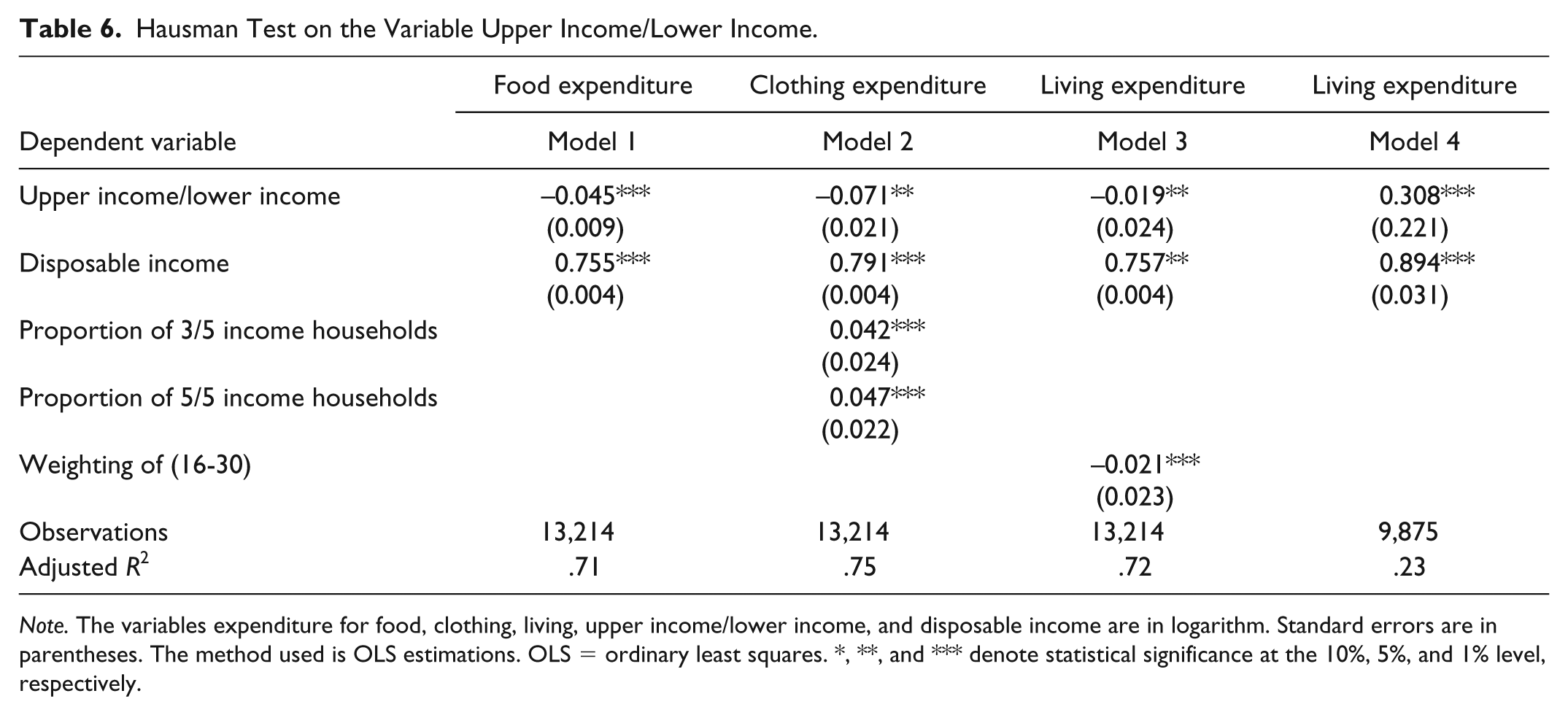
Note. The variables expenditure for food, clothing, living, upper income/lower income, and disposable income are in logarithm. Standard errors are in parentheses. The method used is OLS estimations. OLS = ordinary least squares. *, **, and *** denote statistical significance at the 10%, 5%, and 1% level, respectively.

Conclusion and Discussion

Since 2006, the rural Gini coefficient, the index of inequality, has increased rapidly in China. From the horizontal perspective, the Gini coefficients in the different rural regions of China show the same tendency. We proposed that with increased inequality of income in rural areas, rural residents will compress their living expenditure for the pursuit of social security and the improvement of social status both in relationship to those rural residents with higher incomes, a vertical perspective, and also in relationship to similar type rural households in different rural areas of China, a horizontal perspective. We use the data of the rural household survey of 2006 to 2016 and take the per capita disposable income as a control variable to do the empirical regression analysis. The results show that the gap of rural residents per capita disposable income has a constraining effect on household consumption. China’s Gini coefficient was 0.4387 in 2006 and it rapidly rose to 0.5200 in 2016, the average annual growth rate is 18.53%. The Gini coefficient rapidly increased in rural China and one fourth of the decrease in APC can be explained by the increase in the Gini coefficient and the constraining effect of inequality on consumption in families where the main household income earner is between 16 and 30 years of age. With increase in the Gini coefficient, the human capital investment in rural households has been gradually strengthening. Other possible relevant factors affecting consumption are examined in the data section of the article. To test the effect of other possible factors besides the increase in income inequality, we divided the rural households per capita disposable income into five groups, and we use an index (low-income group/high-income group) to reflect the degree of polarization. In conclusion, the empirical analysis showed that the constraining effect on consumption for living expense in the low-income class is far greater than in the high-income class.

Therefore, by using these two different indexes, the Gini coefficient and polarization between upper and lower income classes, to measure social inequality, we propose that the lower income class will not reduce their investment in health and education just because their disposable income, although rising, slightly is still low. They will not give up the pursuit of social mobility and the possibility to enter a higher social class. This explains why the motivation of consumption has been sinking even though incomes have been rising in China’s rural areas.

Footnotes

Declaration of Conflicting Interests

The author(s) declared no potential conflicts of interest with respect to the research, authorship, and/or publication of this article.

Funding

The author(s) disclosed receipt of the following financial support for the research, authorship, and/or publication of this article: This work was supported by the National Natural Science Foundation of China under Grant 71601002, the Humanities and Social Sciences Foundation of Ministry of Education of China under Grant 16YJC630077, the major project of Humanities and Social Sciences of Ministry of Education of China under Grant 16JJD840008, and the Foundation for Young Talents in College of Anhui Province under Grant gxyqZD2018033.

Notes

Author Biographies

Zengwen Wang has an MSc and a PHD degree in pure mathematics and public administration from Wuhan University, China, respectively. He is a professor in the School of Political Science and Public Administration at Wuhan University and a senior researcher in the Research Center for Social Security Studies at Wuhan University. His research areas are social welfare and economic development, government management decision-making, poverty analysis, and employment. He has authored two books and published more than 60 articles to professional journals including journals such as Journal of Public Management, Symmetry, Journal of Business Economics and Management, Technological and Economic Development of Economy, Complexity, IEEE Access, Journal of Political Science, The Population of China Science, Journal of Chinese Administrative Management, Journal of Chinese Soft Science, and others.

Xiaodi Liu has an MSc and a PHD degree in pure mathematics from Wuhan University, Management Science from College of Economics and Management at Nanjing University of Aeronautics and Astronautics, China, respectively. He is an associate professor in the School of Mathematics and Physics at Anhui University of Technology. His research areas are multiple attribute decision-making, clustering analysis, and aggregation operators. His articles are published by Journal of Business Economics and Management, Technological and Economic Development of Economy, Complexity, Journal of Intelligent & Fuzzy Systems, IEEE Access, Information Fusion, Symmetry, Applied Soft Computing, Journal of Grey System, Mathematical Problems in Engineering, Journal of Intelligent Systems, and others.

References

Bakshi

Chen

(1996). The spirit of capitalism and stock-market prices. American Economic Review, 86, 133-157.

Chunling

(2005). The stratified prestige of contemporary Chinese society occupational prestige and socio-economic status index measurements. Sociological Research, 74(2), 102-106.

Corneo

Jeanne

(1998). Social organization, status and savings behavior. Journal of Public Economics, 70(1), 37-51.

Cowell

(1989). Sampling variance and decomposable inequality measures. Journal of Econometrics, 42, 27-41.

Fang

Wang

(2011). Studies of increasing farmers’ income and expanding rural consumption. Management World, 5, 66-187.

Goldthorpe

J. H.

(2007). On sociology: Critique and program. Stanford, CA: Stanford University Press.

Hausman

J. A.

(1978). Specification tests in econometrics. Econometrica, 46, 1251-1271.

Kotlikoff

L. L.

(1981). The pole of intergenerational transfers in aggregate capital accumulation. Journal Public Economy, 34, 706-732.

Kraay

(2000). Household savings in China. World Bank Economic Review, 14, 545-557.

10.

Kuijs

(2006, July). How will China’s saving-investment balance evolve? (World Bank Policy Research Working Paper No. 3958). Retrieved from https://papers.ssrn.com/sol3/papers.cfm?abstract_id=923265

11.

Martin

(1974). Social security, induced retirement and aggregate capital accumulation. The Journal of Political Economy, 82, 905-926.

12.

Qiang

(1997). Economic stratification and political stratification. Sociological Research, 34(4), 43-55.

13.

Qiang

(2002). Analysis and forecast of Chinese social situation. Beijing, China: Social Science Press.

14.

Saunders

(2017). Social mobility myths. Lanham, MD: Rowman & Littlefield.

15.

Weber

(1922). Economy and society (Translated and reprinted). Berkeley: University of California Press.

16.

Weiss

Fershtman

(1998). Social status and economic performance: A survey. European Economic Review, 42(3), 801-820.

17.

Wen

(2016). Saving and growth under borrowing constraints: Explaining the “high saving rate” Puzzle. (Working papers). Federal Reserve Bank of St. Louis, MO.

18.

(2015). A time series analysis of China rural residents consumption structure based on AIDS model. Statistics & Information Forum, 30(1), 71-75.

19.

Hongbin

Binzhen

(2017). Income inequality and social status seeking. Quarterly Journal of Economics, 29(3), 887-912.

20.

Yuan

Xia

(2017). An empirical analysis of Chinese rural residents’ consumption demand based on QUAIDS model. Studies in Labor Economics, 5(4), 48-81.

21.

Zhang

Zhao

(2017). An empirical study of social welfare affecting rural consumption. Journal of Xi’an Jiaotong University (Social Sciences), 37(142), 100-107.

22.

Zhou