Sage Journals: Discover world-class research

Abstract

Multidimensional scaling (MDS) is a statistical technique commonly used to model the psychological similarity among sets of stimulus items. Typically, MDS has been used with relatively small stimulus sets (30 items or fewer), in part due to the laborious nature of computational analysis and data collection. Modern computing power and newly advanced techniques for speeding data collection have made it possible to conduct MDS with many more stimuli. However, it is as yet unclear if MDS is as well-equipped to model the similarity of large stimulus sets as it is for more modest ones. Here, we conducted 337,500 simulation experiments, wherein hypothetical “true” MDS spaces were created, along with error-perturbed data from simulated “participants.” We examined the fidelity with which the spaces resulting from our “participants” captured the organization of the “true” spaces, as a function of item set size, amount of error in the data (i.e., noise), and dimensionality estimation. We found that although higher set sizes decrease model fit (i.e., they produce increased “stress”), they largely tended to increase determinacy of MDS spaces. These results are predicated, however, on the appropriate estimation of dimensionality of the MDS space. We argue that it is not only reasonable to adopt large stimulus set sizes but tends to be advantageous to do so. Applying MDS to larger sets is appealing, as it affords researchers greater flexibility in stimulus selection, more opportunity for exploration of their stimuli, and a higher likelihood that observed relationships are not due to stimulus-specific idiosyncrasies.

Keywords

multidimensional scaling similarity simulations

Introduction

Multidimensional scaling (MDS) is a statistical technique (see Shepard, 1980; Torgerson, 1958) that is often used to model the psychological similarity among a set of items (see Hout, Papesh, & Goldinger, 2012, for a review). MDS takes as input a set of proximities—that is, estimates of how similar (or dissimilar) each pair of items is to one another—and produces as output a “map” that conveys spatially the relationships among all the stimuli. The distance between any pair of stimuli (or points) in this multidimensional space (the exact number of dimensions used to produce the output is specified by the analyst) is taken as an index of the similarity of the pair, relative to other pairs in the space. As such, stimuli closer in space denotes proportionately more similarity, and vice versa.

Most commonly, MDS is used with relatively small sets of stimuli, often in the range of 10 to 30 items (e.g., Hout, Goldinger, & Brady, 2014). Partly, this is due to the laborious nature of collecting similarity ratings for use in MDS. As the stimulus set increases, the number of comparisons required to perform an analysis grows dramatically; specifically, for n stimulus items, n(n–1) / 2 ratings are required, such that each item is compared with every other at least once. For example, if you have as few as 30 items, 435 pairwise ratings are required; adding only another five items to the stimulus set (35 items) brings the required comparisons up to 595, and a doubling of the original set (60 items) requires a staggering 1,770 ratings. For context, consider for a moment that typical psychological experiments on visual memory routinely use thousands of images (e.g., Brady, Konkle, Alvarez, & Oliva, 2008; Cunningham, Yassa, & Egeth, 2015; Standing, Conezio, & Haber, 1970). Acquiring similarity ratings for 2,000 items would require just shy of 2 million comparisons. Clearly, it would be arduous and time-consuming for research participants to provide so many estimates of similarity. Even 60 items is not an unreasonable amount of stimuli for a researcher to wish to employ in his or her experiment, but such lengthy data collection protocols have often discouraged investigators from modeling similarity for large stimulus sets.

Fortunately, recent alternative approaches for collecting similarity data (that utilize spatial arrangement of the stimuli) have been adopted that drastically speed data collection time (e.g., Goldstone, 1994; Hout & Goldinger, 2016; Hout, Goldinger, & Ferguson, 2013; Kriegeskorte & Mur, 2012; see also Verheyen, Voorspoels, Vanpaemel, & Storms, 2016, for a discussion of the limitations of spatial methods). These methods, coupled with the advent of Internet-based data collection approaches (like Amazon’s Mechanical Turk; see www.mturk.com), which can spread observations across many people, make it quite likely that researchers will soon more frequently conduct MDS analyses on large stimulus sets (see, for instance, Berman et al., 2014, and Horst & Hout, 2016, for scaling of 60-70 items). Applying MDS to larger stimulus sets is very appealing, as it affords researchers greater flexibility and precision in stimulus selection (see Hout et al., 2015 for discussion), more opportunity for exploration of their stimuli, and a higher likelihood that experimentally observed relationships are not due to stimulus-specific idiosyncrasies. Moreover, modern uses of MDS have expanded beyond directly observing similarities (e.g., by asking human participants to provide ratings) to deriving them from secondary sources, such as functional magnetic resonance imaging (fMRI) data (see Mair, Borg, & Rusch, 2016, for discussion of “directly observed” vs. “derived” proximities). When such approaches are adopted, the number of to-be-scaled “points” can number in the hundreds to thousands. Thus, it seems more important than ever to understand fully how well MDS can handle such rich data sets.

MDS clearly has a long and important history of adoption in the psychological literature (see Nosofsky, 1986; Shepard, 1987; Shepard, 2004), and its utility is widely accepted. However, it remains unclear whether MDS is as well-equipped to model the similarity of large stimulus sets with the same precision as it is with more modest ones (see the General Discussion for examples of algorithms designed specifically to reduce computational complexity when used with large set sizes). Determining the appropriate dimensionality (i.e., the number of coordinate axes used to locate the points in space) of the space is no trivial matter (see Lee, 2001; Oh, 2011), and as such, it is further unclear what effect the under- or overestimation of dimensionality will have upon the quality of the modeled distances (but see Sherman, 1972). It could be the case that when burdened with many items, MDS analyses deteriorate, and provide an output that simply reflects noisy variation. It may also be the case that under- and overestimation of dimensionality have asymmetric effects on the quality of the output. These are difficult questions to examine empirically, because MDS most commonly deals with inherently subjective similarity ratings that, by their very nature and design, are subject to individual differences. Moreover, objective measures of model fit, such as stress (which quantifies the extent to which the MDS solution reflects its raw inputs), are responsive to aspects of the design that are not necessarily reflective of the quality of the data (e.g., stress necessarily increases with larger set sizes; see Isaac & Poor, 1974; Spence & Young, 1978). Although a full review of MDS is beyond the scope of this article, interested readers can find in-depth reviews and tutorials in Borg and Groenen (1997); Giguere (2006); Green, Camone, and Smith (1989); Hout et al. (2012); Jaworska and Chupetlovska-Anastasova (2009); Kruskal and Wish (1978); and Shiffman, Reynolds, and Young (1981).

In the current investigation, we sought to examine the extent to which MDS is capable of handling large stimulus sets using a series of simulation studies. In our simulations, we randomly created hypothetical “true” multidimensional spaces. We next simulated participant-level data by adding multivariate normally distributed error to the true locations. These noisy data were subsequently subjected to an MDS analysis. Our goal was to examine the fidelity with which the space resulting from our simulated participants captured the organization of the “true” spaces. We performed these simulations across a range of dimensionalities, and most importantly, for varying set sizes numbering as high as 1,024 items.

Our data were scaled using metric MDS (which takes as input interval or ratio scale similarity estimates), rather than nonmetric MDS (which takes as input ordinal scale data). We did this for two reasons: First, interval and ratio-level data are quite commonly collected in psychology experiments when similarity ratings are provided by human participants. For instance, a participant may be shown stimuli two at a time, and be asked to indicate the similarity of the pair using a “slide-bar” (which may be converted, for example, to a rating of 0-100), or a group of participants may be shown a full set of stimuli and be asked to sort the items into piles based on their similarity (in which case the input data are the proportion of independent raters who grouped each pair of stimuli together). Perceptual discrimination tasks are also commonly employed, whereby participants are asked to indicate whether a pair of stimuli are the same or different; in such cases, the input data take the form of discrimination response times, or the proportion of discriminations errors committed across participants. The second reason for performing metric MDS is that spatial methods of collecting similarity estimates are particularly advantageous when collecting data on many stimulus items, and spatial proximities are most commonly collected in the form of Euclidean distance.

In Experiment 1, our simulated data were scaled in the correct dimensionality from which the “true” space was created (e.g., simulated data were scaled in three dimensions when the “true” space was generated using three dimensions). In Experiment 2, we systematically underestimated the dimensionality of the space (e.g., scaling in two dimensions when the “true” space was created from three), and in Experiment 3, we systematically overestimated the dimensionality of the space (e.g., scaling in four dimensions when the “true” space was created from three). In sum, our findings indicate that MDS can adequately handle large set sizes, and that rather than degrading, the quality of the solutions tends to increase as the set size increases. Importantly, however, such findings are not universal, and depend not just on the number of items in the space or the amount of noise in the data, but also on whether the dimensionality of the space is underestimated, correctly estimated, or overestimated.

Our simulations contain a family resemblance to very early work by Young (1970), who made the first attempt at answering this question by simulating data for up to 30 items. Although this previous work laid the foundation for our own, the current studies build upon it in the following ways: (a) we extended the stimulus set sizes beyond 1,000 items, establishing that the observed results are consistent, and encompass a range of stimulus set sizes that are of interest to modern day MDS users; (b) by performing these simulations many thousands of times, we show that our results are not the convenient outcome of a single, fortunate simulation; and (c) we show that this large set benefit is contingent on the proper selection of dimensionality for the space, and that when the dimensionality of the solution is over- or underestimated, larger set sizes can sometimes be detrimental to the quality of the solution.

Assessing the Quality of MDS Data

Is it possible to assess the quality of an MDS solution outside of the simple, set size-dependent analysis of model fit (i.e., “stress”)? Although there is no method by which the “true” underlying structure of a space may be revealed (Goldstone & Medin, 1994), the quality of the data can be inferred by less direct means. One way to accomplish this is to artificially create stimuli with well-controlled perceptual dimensions, and then examine the extent to which an MDS analysis reveals these prescribed features. Hout et al. (2013; Experiment 1) created artificial stimuli, using equivalent and (arguably) equidistant feature levels. Stimuli were simplistic “spokes” and “bugs” that varied in line width, spoke angle, and color, or in antennae curvature, number of legs, and body coloration (for spokes and bugs, respectively). The goal was to compare and contrast how well various methods of collecting similarity ratings (e.g., traditional pairwise, spatial arrangement method, or SpAM) recovered the multidimensional organization of these unsophisticated (and uncontentious) stimuli.

A second approach is to examine the ability of MDS data to predict psychologically meaningful behavior, such as the ability to discriminate between two visually similar icons. In Hout et al. (2013; Experiment 3), MDS ratings were collected for the artificially created bug stimuli, and for novel, computer-generated faces (that varied in skin tone and degree of separation between the eyes). Participants were then given a pair of “same/different” discrimination tasks. In the speeded version of the task, people saw a pair of pictures on each trial (simultaneously presented), and as quickly as possible indicated if the pair were the same or different. In the unspeeded version of the task, people saw one picture, briefly presented, followed by a noisy backward-mask, and then a second (briefly presented) picture. They then indicated if the pictures were the same or not, but were encouraged to strive for accuracy, rather than speed. To determine how well the MDS spaces recovered the psychological spaces for the bug and face stimuli, generalization gradients were created (see Shepard, 1957; Shepard, 1958; Shepard & Chang, 1963) using the interitem distances for every pair of pictures (i.e., the distance in MDS space) to predict discrimination reaction times and accuracy (for the speeded and unspeeded tasks, respectively). Quality of the MDS solutions was then quantified using the variance accounted for by each generalization gradient.

These approaches were fruitful in examining the quality of data for relatively few (and simple) stimuli, but their adoption for larger stimulus sets would be extremely labor-intensive, and inefficient. A third alternative is offered by Young (1970; following similar approaches by Kruskal, 1964, and Shepard, 1966), who used Monte Carlo simulations to investigate the quality of MDS data as a function of stimulus set size, error, and dimensionality (for analogous Monte Carlo simulation studies, see also Cohen & Jones, 1974; Isaac & Poor, 1974; Sherman, 1972; Spence & Ogilvie, 1973; Stenson & Knoll, 1969). Young (1970) started with “true” configurations that had been previously generated by randomly creating point coordinates in multidimensional space (taken from Coombs & Kao, 1960). He then generated distances that included error variation, derived from the “true” distances in hypothetical space. These data were subjected to MDS analysis to determine how well the error-perturbed data recovered the “true” organization of the points. Young’s (1970) findings indicate that the precision of the resulting MDS space decreases with more error in the ratings and with higher dimensionality of the space, but more interestingly, that it increases with more items in the space.

This seminal work provides a theoretical grounding for the current investigation, and in our studies, we conceptually replicated this technique. However, the Young (1970) study suffers several shortcomings that merit mentioning, for they call into question the generalizability of the findings. First, simulations were performed for only as many as 30 stimulus items. Second, the simulations were only replicated 5 times. Certainly, these two limitations were likely a direct consequence of the computational demands required to perform such an onerous analysis prior to the advent of modern computing. Third, these simulations assumed that the analyst correctly determined the dimensionality of the “true” multidimensional space. As such, further work is warranted to establish the reliability of these findings across a wider range of stimulus set sizes, across a larger set of replications, and for situations in which dimensionality of the space is improperly determined. In the current investigation, we accomplish all of these things by performing simulations for over a 1,000 stimulus items, by replicating our simulations many thousands of times, and by including simulations that systematically over- or underestimate the dimensionality of the MDS space.

Experiment 1

In our first set of simulations, we created hypothetical spaces for up to 1,024 items in multidimensional space, across a range of dimensionalities (2-6), and scaled the data using the correct dimensionality from which the “true” space was generated. Our simulated participant-level data were created by adding normally distributed noise to the coordinate locations of points in the “true” space. This is conceptually akin to individual participants randomly (and independently) over- or underestimating the similarity of pairs of stimuli. More specifically, we simulated error variation by manipulating the standard deviation of the distribution from which our noise levels were sampled. Ten simulated participants were created for each combination of item set size, dimensionality, and error level. We chose a sample size of 10 for our simulations because that sample size is common in cognitive psychology experiments, and we wanted to match the number of participants closely to typical conditions in the lab. In addition, we had no a priori reason to suspect that our simulations would be any different with more simulated participants. There were 135 total combinations of those factors, and each simulation was conducted 500 times, yielding a total of 67,500 simulations in Experiment 1.

Method

Design

We simulated MDS spaces and error-perturbed data that varied in error variability, dimensionality, and number of items in the space, creating a 3 × 5 × 9 design: Error Level (1, 5, 10 unit standard deviation noise distributions), Dimensionality (2-6), and Number of Items (4, 8, 16, 32, 64, 128, 256, 512, 1,024).

Simulations

All simulations were conducted using MATLAB (“MATLAB and Statistics Toolbox Release,” 2015). Data were analyzed using MATLAB’s mdscale function, which was used to perform metric MDS (more specifically, ratio MDS) to produce distance estimates at a specified dimensionality. Example MATLAB code demonstrating the details of the simulations is included in the Appendix. The steps for conducting the simulations were as follows:

Step 1: Values were selected for the number of items (n; 4, 8, 16, 32, 64, 128, 256, 512, 1,024), the “true” dimensionality (k; 2, 3, 4, 5, 6), the assumed dimensionality of the MDS analysis (m; 2, 3, 4, 5, 6), and Error Level (s; 1, 5, or 10 units). For Experiment 1, the assumed dimensionality was always equal to the “true” dimensionality (but for Experiments 2 and 3, assumed dimensionality was systematically under- or overestimated, respectively).

Step 2: The “true” locations of n items in k-dimensional space were randomly generated. These locations served as the “truth” for the 500 simulated experiments conducted in Step 3. Each coordinate was sampled from a uniform [–5, 5] distribution. For example, in a two-dimensional space, coordinates for x and y were each sampled from a [–5, 5] uniform distribution. Because the uniform distribution was 10 units wide, the variance of the coordinates was 8.33, and the standard deviation of the coordinates was 2.89.

Step 3: For each of the 500 simulated experiments, normally distributed noise with a mean of zero and standard deviation equal to s was added to each true coordinate to produce data from 10 different simulated participants. For example, consider object p whose true location is at (x_p, y_p) in two-dimensional space. The location of this object for subject i, denoted as (x_ip, y_ip), was simulated as

(x_{i p}, y_{i p}) = (x_{p} + e_{i x}, y_{p} + e_{i y}),

where e_x and e_y are independent samples from a normal distribution with mean zero and standard deviation s. The Euclidean distances between the n(n–1) / 2 pairs of objects in the space were then calculated for each simulated participant. For each pair of points, the mean distance (averaged across the 10 simulated participants) was then calculated and used as input to the MDS analysis.

Step 4: Metric MDS analyses were then conducted using squared stress as the criterion, with dimensionality equal to k. MATLAB’s mdscale function was used to conduct the MDS analyses, and the metricsstress parameter was used to enable metric scaling. This parameter causes the mdscale function to perform metric MDS using squared stress normalized by the sum of the fourth powers of the dissimilarities as the criterion:

\frac{\sum \sum {(x_{i j} - d_{i j})}^{2}}{\sum \sum {(x_{i j})}^{4}},

where $x_{i j}$ is the input dissimilarity between objects i and j, and $d_{i j}$ is the Euclidian distance between objects i and j in the map that results from the MDS analysis. From this analysis, our dependent variables (explained below) were calculated. Results were averaged across the 500 experiments to obtain values for each combination of n, k, and s.

Results

The reporting of our results includes a pair of dependent variables which require brief explanation. We first report interitem distance vector correlations, which index the amount of agreement between the distances in the “true” spaces and those in the reconstructed, error-perturbed MDS solutions. High correlations indicate that pairs of points that are located close to one another in the “true” space are close together in the reconstructed space, and vice versa (see Hout et al., 2013, or Goldstone, 1994, for documented examples of this analysis approach). Hereafter, following Young (1970), we will refer to this as “determinacy” (i.e., the degree to which the MDS solutions determined the correct organization of points). We report R² rather than the Pearson Product-moment correlation coefficient for easier interpretation of our results in terms of the amount of variance accounted for. We next report the interitem distance vector correlations between the “true” spaces and our raw, participant-level data (i.e., data matrices that have not yet been subjected to MDS); hereafter, we will refer to this as “correspondence” (i.e., the degree to which the raw simulated data points correspond with the “true” multidimensional distances). We report these correspondence values simply to demonstrate that our main finding of interest—the degree to which MDS recovers a similarity space with greater fidelity as the number of points in the space increases—is not a mathematical inevitability. That is, it is not due to an error in the simulations which may have caused a greater correspondence between “true” spaces and individual participant-level ratings at higher stimulus set sizes.

It bears brief mention that we do not report stress values in our results. It is already well-established that stress values increase in response to added noise and increased stimulus set size, and decrease in response to increased dimensionality of the space (see, for instance, Isaac & Poor, 1974). Because the stress values in our data followed previously documented, systematic patterns, we chose not to report them in the interest of brevity.

Determinacy

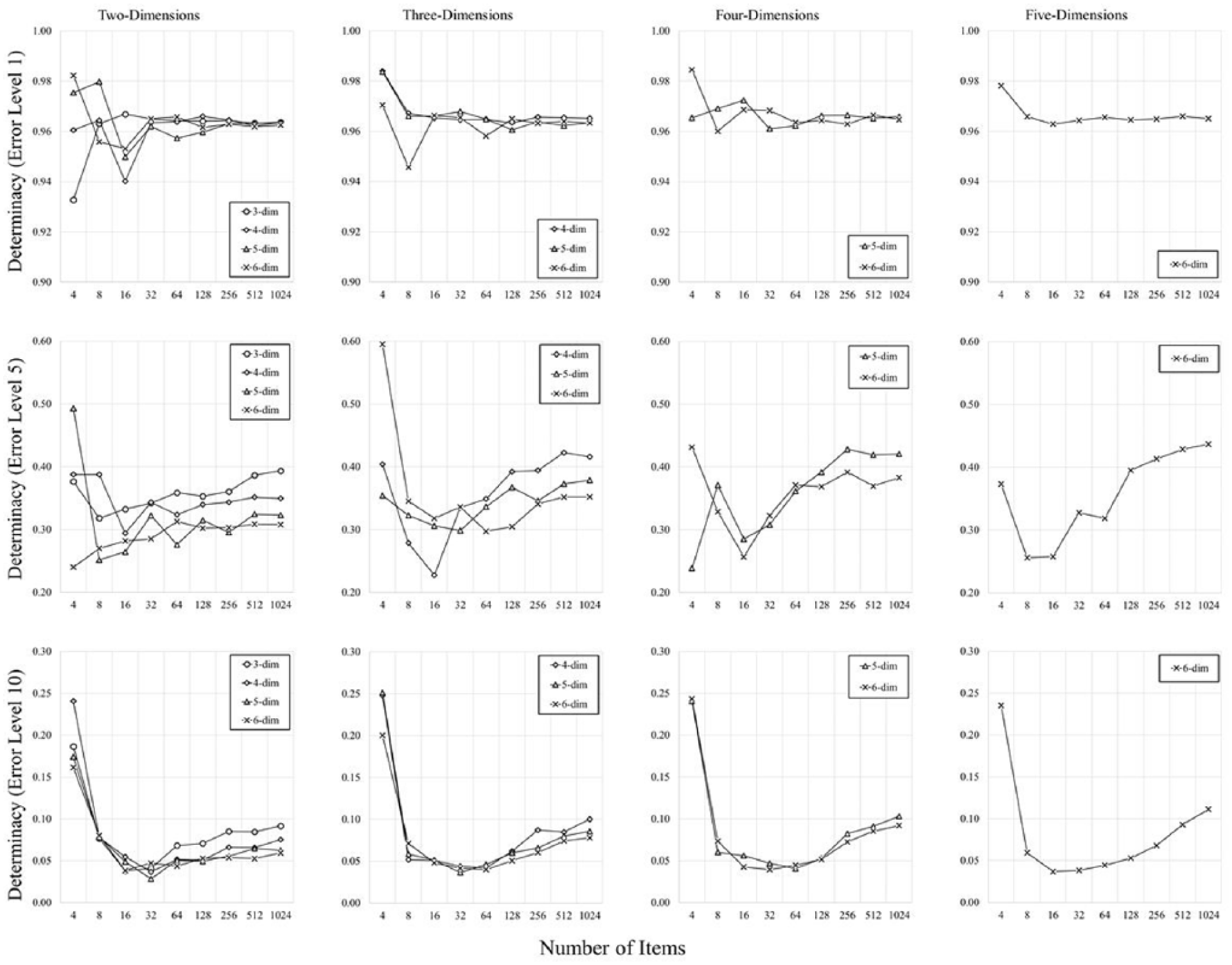
Figure 1 shows the determinacy values for each of our simulations. Determinacy is hindered by added noise (evidenced by the differing range of the y-axes moving from left to right panels), but is relatively unaffected by higher dimensionality (evidenced by the lines resting more or less atop one another throughout). Critically, at low-levels of error, determinacy is high, and presents a relatively steady relationship with the number of items in the space, but when error levels are higher, this relationship begins to change in a nonlinear fashion. At small set sizes, determinacy is somewhat less systematic and seems, if anything, to decrease with more items in the space. This is a trend consistent with Young’s (1970) data, and it is not surprising, as correlations at set sizes of four and eight are only derived from a collection of six and 28 pairs of points, respectively. It seems clear, however, that when moving beyond 16 items, determinacy begins to reliably increase as more items are added to the space.

Figure 1.

Determinacy (reported as proportion of variance accounted for) presented as a function the number of items, error level (increasing across panels from left to right), and dimensionality (shown using different symbols), from Experiment 1.

Correspondence

Figure 2 presents the correspondence between the raw simulated distances (i.e., the proximities averaged across our simulated “participants,” prior to being subjected to MDS), and the “true” distances in multidimensional space. In keeping with the design of the simulations, the correspondence was lower for higher error rate data (moving across panels from left to right). More importantly, there was clearly no beneficial relationship between the degree of correspondence and the number of stimulus items in the space. Indeed, the opposite was true, in that more items in the space tended to lead to worse correspondence, particularly for higher levels of error. This finding simply represents a “sanity check” for our simulations, indicating clearly that the relationship between observed determinacy and the number of items was not mathematically inevitable. Having more items in the space did not mean that participant-averaged raw data were more likely to resemble the “true” spaces. Instead, increased determinacy (as a function of the number of items in the space) came about when participants’ data were transformed through MDS to give rise to an aggregate solution.

Figure 2.

Correspondence (reported as proportion of variance accounted for) between raw participant-level data and the “true” distances in multidimensional space, from Experiment 1.

It may be observed that in places the variance accounted for in determinacy (shown in Figure 1) is less than that of the variance accounted for by correspondence (shown in Figure 2). Importantly, substantial numerical advantages from correspondence only arise when the number of stimuli is quite low, or when the error level is large. In practice, MDS would likely not be performed on so little stimuli, nor would the analyst choose to scale data that she or he presumed to have such a high level of error variation. Importantly, the central message of Experiment 1 holds, namely, that determinacy tends to increase with more stimuli, and not because correspondence is increasing at larger set sizes.

Discussion

In Experiment 1, we provided evidence that the fidelity of the spaces recovered by MDS increases when more items are present in the space. These findings, however, assume that the analyst correctly determined the dimensionality of the space when scaling the data. In Experiment 2, we explore the effects of systematic underestimation of dimensionality.

Experiment 2

Our second round of simulations were identical to the first, save one important factor. Now, rather than assume the analyst correctly identified the dimensionality of the space, we explore what happens when dimensionality is improperly underestimated. As such, we now present the results separately as a function of the “true” dimensionality (3, 4, 5, or 6), and the estimated dimensionality (2, 3, 4, or 5). Because different levels of dimensionality inherently have an unequal number of dimensions by which they can be underestimated, it is no longer possible to envision a factorial design, as in Experiment 1. Rather, results are plotted for every possible underestimation (e.g., for two assumed dimensions when the “true” dimensionality was three; for two, three, four, and five assumed dimensions when the “true” dimensionality was six). This yields 270 combinations of “true” dimensionality, assumed dimensionality, number of items in the space, and error level. As in Experiment 1, each simulation was conducted 500 times, yielding a total of 135,000 new simulations in Experiment 2, again with 10 simulated participants each.

Method

The methods of Experiment 2 were identical to Experiment 1, save the fact that the MDS solutions were no longer scaled in the appropriate “true” dimensionality (denoted as k). Rather, they were systematically underestimated for dimensionalities of three through six, using every possible underestimation (i.e., two through five). In other words, the true dimensionality k was either 3, 4, 5, or 6, and the assumed dimensionality m was set to values 2, 3, 4, and 5 such that m < k.

Results

In Experiment 2, we again present results for determinacy. However, we no longer present any correspondence data. Correspondence values represent the correlation between raw, unscaled “participant” data and the “true” distances in multidimensional space. Thus, exploring underestimation of dimensionality (the sole purpose of Experiment 2) would have no bearing on correspondence, and thus correspondence is no longer informative. No correspondence is reported for Experiment 3 for this same reason.

Determinacy

Figure 3 presents the determinacy values for our simulations. As in Experiment 1, determinacy is (not surprisingly) hindered by added noise, which can be appreciated by noting the different ranges of the y-axes moving down the rows of panels. Also in keeping with Experiment 1, determinacy is relatively unaffected by increasing “true” dimensionality, which can be appreciated by noting that the range and “center of gravity” of the plots is more or less equivalent when moving across columns (within rows). It may be noted that determinacy is now lower, relative to Experiment 1 (see Figure 1). This is to be expected, as the simulations in Experiment 2 were scaled using fewer dimensions than are necessary to represent all the proximity information.

Figure 3.

Determinacy presented as a function the number of items, error level (increasing down rows from top to bottom), “true” dimensionality (increasing across columns from left to right), and assumed dimensionality (shown using different symbols), from Experiment 2.

More importantly, determinacy again shows a nonlinear relationship with the number of items in the space. When the dimensionality of the space is underestimated, determinacy trends downward universally, provided the error rate is low (i.e., the top row of panels). When the error rate increases (i.e., middle and bottom rows of panels), however, roughly U-shaped functions begin to emerge, whereby increasing the number of items in the space is a hindrance up to around 16 items, but thereafter, determinacy either begins to plateau, or in some cases to increase as more items are added to the space.

Discussion

In Experiment 2, we explored the effects of systematic underestimation of dimensionality, finding a more nuanced story than Experiment 1, wherein dimensionality was correctly estimated. We again found nonlinear relationships between determinacy and the number of items in the space. When error levels were low, adding items to the space was universally detrimental to determinacy, but at higher rates of error, determinacy was only hindered by more items when the total number of items was quite low (e.g., around 16 or fewer). It bears repeating here that when set sizes are so low, correlations can be unstable, as they are based on a small number of observations. When the space contained a greater number of items, however, determinacy was largely unaffected by increasing numbers of items, and in some cases was even helped by their presence. In Experiment 3, we come full circle by next exploring the effects of systematic overestimation of dimensionality.

Experiment 3

Our final round of simulations was identical to the second, except that we now explored what happens when dimensionality is improperly overestimated. Again, a factorial design was not possible, so results are plotted for every possible overestimation (e.g., for three, four, five, and six assumed dimensions when the “true” dimensionality was two; for six assumed dimensions when the “true” dimensionality was five). This yielded another 270 combinations of “true” dimensionality, assumed dimensionality, number of items in the space, and error level. Each simulation was again conducted 500 times (with 10 simulated “participants” each), producing 135,000 new simulations in Experiment 3.

Method

The methods of Experiment 3 were identical to Experiment 1, save the fact that the MDS solutions were no longer scaled in the appropriate “true” dimensionality (denoted as k). Rather, they were systematically overestimated for dimensionalities of two through five, using every possible overestimation (i.e., three through six). In other words, the true dimensionality k was either 2, 3, 4, or 5, and the assumed dimensionality m was set to values 3, 4, 5, and 6 such that m > k.

Results

As in Experiment 2, we report results for determinacy as a function of each possible factor.

Determinacy

Figure 4 shows the determinacy values for our final simulations. As in Experiments 1 and 2, determinacy was hindered by added noise (evidenced by the changing range of the y-axes moving down the rows), and in keeping with Experiment 2, was relatively unaffected by increasing “true” dimensionality (evidenced by a relatively constant “center of gravity” across columns within each row).

Figure 4.

The critical finding here is that determinacy once more presented with a nonlinear relationship to the number of items in the space. It should be noted that overall, unlike when dimensionality was underestimated, overestimation of dimensionality results in almost no negative effect of increasing numbers of items in the space. When the error level is low (i.e., the top row of panels), determinacy is more or less flat as a function of the number of items in the space. When error increases (i.e., the middle and bottom rows of panels), the U-shaped functions reemerge. At small item amounts (~4 to 16), more items seem detrimental to determinacy, but moving beyond 16 items, determinacy seems to benefit steadily from an increase in the number of items in the space.

Discussion

In Experiment 3, we rounded out our investigation by exploring the effects of overestimation of dimensionality, finding a story largely in line with Experiment 2 (where dimensionality was underestimated), but far more positive as concerns the ability of MDS to recover the “true” underlying organization of the space. The observed nonlinear relationships (at the more substantial error levels) suggest once more that when item set sizes are reasonably large, adding more items to the space aids determinacy more than it hurts. Indeed, the observed relationships in Experiment 3 (beyond 16 items) tended to remain flat (when error was low), or to steadily increase (when error was greater). Once more, the less consistent relationships shown when stimulus set sizes were low is to be expected, due to the small number of observations used to determine the correlations. Taken together, this suggests that at best, increasing the number of items is helpful when dimensionality is overestimated, and at worst, it is not harmful.

General Discussion

In this investigation, we conducted 337,500 simulated experiments to investigate the extent to which MDS spaces are affected by the addition of more items in multidimensional space. Specifically, we explored how determinacy was affected by the number of items in the space, and the extent to which these findings interacted with the amount of error in the input ratings, the “true” dimensionality of the space, and the degree to which the dimensionality of the space was improperly estimated. Taken together, our most important findings suggest that increasing the number of items in the MDS space does not overwhelm the iterative process by which items are “moved” into the appropriate location in multidimensional space (relative to one another). Instead, overall, increasing the number of items in the space seems to provide a benefit, by increasing the degree to which the organization of the space resembles the “true” organization of points.

However, these simulations also make clear the importance of correctly estimating the dimensionality of the space. When dimensionality was underestimated and error was low, adding items to the space was detrimental to determinacy, and only when error levels were higher did increased items seem to provide a benefit (i.e., once the items numbered greater than 16). By contrast, determinacy was more positively affected when dimensionality was overestimated. At low levels of error, adding items to the space had no consistent effect on determinacy, but at higher error levels, more items in the space provided a universal benefit once the items exceeded around 16. It seems clear, therefore, that—considering human provided similarity ratings are prone to noisy variation—it might be best (when using large stimulus item sizes) to err on the side of overestimation, rather than underestimation of dimensionality. Indeed, such a conclusion is consistent with earlier work by Sherman (1972), who in a series of conceptually similar Monte Carlo simulations concluded that overestimation of dimensionality is more likely to yield a successful MDS solution than underestimation.

Why Do Larger Set Sizes Increase Determinacy?

Why might larger set sizes increase the fidelity of data produced by a MDS analysis? MDS is an iterative process that takes into consideration a complex set of interrelationships among stimuli, therefore it would not be unreasonable to suppose that a greater number of stimuli could become a burden to the analysis. Instead, what we found is that something akin to the law of large numbers (i.e., as sample size grows, the mean of a sample will become closer to the true population value) is acting upon the placement of items in the space. Intuitively, this explanation makes sense. The location of a single stimulus item in multidimensional space is determined by the proximities (i.e., similarity ratings) between the item in question and every other item in the space. Specifically, for an MDS space with n items, each stimulus is located using n–1 proximities. Thus, as n increases, so too does the amount of information that determines where the item will be placed.

To elaborate, MDS is not singly deterministic: That items A and B are given a similarity rating of X does not mean that item A will be placed in any particular coordinate location determined by X. Instead, the placement of item A is determined by its relationship with items B, C, D, and so on. In effect, it is “pushed” and “pulled” into position by its relationship with all the other items in the space. When there are more items in the space, therefore, there is more opportunity for item A to be located in a position that most accurately reflects its relationship among all the points. For example, if item A is initially located too close to item B, its location may be further tuned by being “pulled” back into position by its relationship with item C, or “pushed” along a different coordinate axis by its relationship with item D, and so on. When one considers the placement of all stimulus items, therefore, it becomes clear that at higher set sizes, heavily perturbed pairwise ratings are more likely to be tempered by the relationships of the stimulus with the other items in the space.

It is important to note that this “law of large numbers effect” is not operating at the level of individual participant ratings. Having participants provide ratings on more stimuli does not increase the fidelity of their raw data, as demonstrated by the correspondence analyses in Experiment 1. The number of stimuli in a space has no beneficial effect on the correspondence between the raw pairwise similarities and “true” distances in multidimensional space. Only once the pairwise ratings have been transformed by MDS do we observe a benefit (at higher set sizes) to determinacy. Because participant-level raw ratings may be imprecise, regardless of stimulus set size, any imprecision may cause stress to increase dramatically with larger set sizes (due to the cumulative stress accruing over many ratings). Importantly, however, this does not appear to come at the expense of the determinacy of the space, because overall determinacy is affected by more than just singular, error-prone ratings. Moreover, having more stimuli in the space is not universally beneficial, even after the ratings have been subjected to MDS. The accurate honing of coordinate locations for items is contingent on an appropriate estimation of the dimensionality of the space.

An analogy may be warranted here to simply convey the benefit of large stimulus set sizes. Imagine a simple, three-dimensional structure that is comprised of a series of joints and girders. Each joint represents a stimulus item in multidimensional space, and each girder represents the similarity rating between a pair of items. For a fixed volume of space, structures with more joints (i.e., MDS spaces with more items) are inherently more stable. This is because with few joints, the destruction (or misplacement) of a single joint can be hugely detrimental to the stability of the structure. When there are many joints, however, if a single joint is in some way damaged or suboptimal, the remaining joints can help to keep the structure secure. In MDS, this is akin to the existence of many (or fewer) stimulus items in the space. When there are more stimulus items in the space, the relationships among all the items appears to support the overall structure of the solution.

Three Historical Concerns About Large Set Sizes (Relieved), and Three Caveats of Which to Be Aware

Historically, MDS analyses have often been conducted on stimuli in the range of 10 to 30 items. There are three potential reasons for the adoption of these relatively small stimulus set sizes: computational effort, data collection time, and concerns about the fidelity of the data. First, to address computational effort: Prior to the advent of modern computing, it would have been prohibitively time-consuming to perform an analysis on more than 30 items, but modern computing makes performing MDS on many thousands of items a trivial pursuit. Performing an MDS analysis on more than a 1,000 items now takes mere seconds with the algorithm employed in the current investigation (i.e., mdscale implemented in MATLAB computing software). Indeed, although the studies presented here focused on stimulus set sizes within the range of around 1,000 items—primarily because it is reasonable to assume that human raters could provide as many proximities—MDS is sometimes conducted on data not provided by human raters, and on a scale far exceeding that of our simulations. In cases with extremely large set sizes, computational speed is at a premium, and as such, modern techniques have been developed specifically to deal with large data sets (see Cox & Cox, 2008 for discussion).

For example, Strickert, Teichmann, Sreenivasulu, and Seiffert (2005) have created a new MDS algorithm called High-Throughput Multidimensional Scaling (HiT-MDS) that was developed specifically for large sample sizes. Their work applied this new algorithm to the study of gene expression, and involved 12,000 different genes. More recently, Vankrunkelsven, Verheyen, De Deyne, and Storms (2015) used HiT-MDS to obtain MDS spaces for over 3,000 stimuli (proximities were derived from the similarity of word pairs, taken from a word association corpus). HiT-MDS is not alone, either. Other methods for tackling the problem of high computational complexity include Fast Spring Model-Visualization (Morrison, Ross, & Chalmesrs, 2003), nonlinear mapping using neural networks (Agrafiotis, Rassokhin, & Lobanov, 2001), majorization algorithms (de Leeuw, 1977) that can be implemented in the R stats package (R Core Team, 2012), spectral MDS scaling (Aflalo & Kimmel, 2013), and split-and-combine MDS (SC-MDS; Tzeng, Lu, & Li, 2008).

Second, to address data collection time, the number of pairwise comparisons required to fill a similarity matrix skyrockets as the stimulus set size increases (see Figure 5, left panel). At four items, only six comparisons are needed, but at 1,024 items, more than half a million comparisons are required. Although this is still a nontrivial concern, modern spatial methods of data collection (e.g., Goldstone, 1994; Hout et al., 2013) and Internet-based data collection techniques (e.g., MTurk; see www.mturk.com) make acquiring data for large stimulus sets a real possibility at present.

Figure 5.

Here are shown the manner in which three variables change as a function of stimulus set size.

Third, to address concerns about the fidelity of the data: In this investigation, we have provided strong evidence that analysts need not be overly concerned that larger stimulus sets will be less deterministic. In fact, we have shown quite the opposite that larger set sizes tend to produce data with better determinacy than those of smaller set sizes, provided the dimensionality of the space is properly estimated, or that the analyst err on the side of overestimation.

Bearing this in mind, there are three caveats of which to be aware when using larger stimulus set sizes. First, as shown in Experiments 2 and 3, when large set sizes are used, incorrect estimation of the dimensionality of the space can cause a serious detriment to determinacy. Great care should be taken to ensure that the MDS space is derived with the appropriate number of dimensions; our simulations suggest that it is less deleterious to overestimate dimensionality than it is to underestimate it. Second, as with any experimental investigation, lengthy experimental protocols can create nonuniform individual differences variation. If an experimenter requires a single participant to rate pairs of stimuli for many hours, obvious concerns about fatigue, boredom, lack of engagement, and shifting strategies on the part of the participant may arise over time. Care should be taken to ensure that the quality of the data is consistent across ratings by, for instance, breaking up large data collection procedures into several experimental sessions, by splitting the ratings across participants, and so on. Third, as outlined above, when using larger set sizes, more information is provided for the placement of each item in multidimensional space. However, there is a nonlinear relationship between the information obtained per item and the amount of information provided per unit time.

This is easily appreciated by examining Figure 5. In the left panel, we show that the number of pairwise comparisons required for an MDS analysis grows sharply as a function of stimulus set size. In the middle panel, we plot the simple, linear relationship between set size and the amount of information provided per item (i.e., the number of pairwise ratings that contribute to the placement of each item). In the right panel, we calculated ratio scores that consider the amount of information provided for each item, scaled by the number of comparisons required to fill a similarity matrix for the given set size. This can be thought of as a cost ratio, taking information obtained (for each item) and dividing it by the total number of similarity ratings that would be required to obtain that information for each item. Here, we see that the cost ratio drops sharply moving toward stimulus set sizes of 100, and plateaus thereafter. This suggests that beyond a certain point, the amount of information you obtain with large set sizes may begin to be outweighed by the amount of time required to obtain the similarity ratings in the first place.

Conclusion

In the past, large (i.e., more than 30 items) MDS experiments were not typically conducted, and for good reason. However, the time is right to start collecting MDS data for larger and larger stimulus sets. We no longer need be concerned about computational power, new techniques of collecting similarity data are speeding up experimental protocols (e.g., Hout et al., 2013; Kriegeskorte & Mur, 2012), and the results of our simulations clearly demonstrate that there is often a determinacy benefit to scaling more items. We suggest that there are three reasons that researchers should strive to conduct MDS analyses with larger stimulus set sizes (in addition to enhanced determinacy). First, when MDS is being used to explore and control stimulus selection, larger set sizes will afford greater experimental flexibility. Second, when MDS is used in an exploratory fashion, additional stimuli may provide more information about the featural dimensions on which the stimuli were rated. And third, by utilizing a larger set size, the conclusions drawn from an MDS solution are less likely to be due to stimulus idiosyncrasies.

Indeed, some researchers are already beginning to adopt larger set sizes. Horst and Hout (2016) had human raters provide similarity ratings for 64 novel objects, and Berman et al. (2014) had human raters provide ratings for 70 pictures of nature. Taken together, alongside the proliferation of algorithms designed to tackle high computational complexity, it seems clear that experimenters and analysts are beginning to move in this direction, and the current work suggests strongly that it is indeed prudent and safe to do so, provided the appropriate care is taken with respect to dimensionality estimation. Of course, the choice of how many stimuli to adopt will vary widely across experimental scenarios. Our hope is that researchers will no longer be hesitant about the quality of their data when using large stimulus set sizes. Each experimenter will now simply need to weigh the pros (e.g., better determinacy, more experimental flexibility) against the cons (e.g., greater data collection time, higher cost ratio) of using many stimuli when deciding how best to conduct their research.

Footnotes

Appendix

Acknowledgements

The authors would like to thank Steven Verheyen for helpful comments during the creation of this article, and for pointing us to important literature. We also thank Matthew Oberdorfer, Alejandrina Garcia, Amelia Selph, and Katrina Ling for assistance in data processing.

Declaration of Conflicting Interests

The author(s) declared no potential conflicts of interest with respect to the research, authorship, and/or publication of this article.

Funding

The author(s) disclosed receipt of the following financial support for the research, authorship, and/or publication of this article: Grant support provided by National Institutes of Health (National Institute on Deafness and Other Communication Disorders) SC1DC016452 to Justin MacDonald.

Author Biographies

Michael C. Hout is an assistant professor in the Department of Psychology at New Mexico State University, and an associate editor at the journal Attention, Perception, and Psychophysics. His research focuses primarily on visual cognition (including visual search, attention, eye movements, and memory) and the development of alternative methods of collecting similarity data for use in multi-dimensional scaling.

Corbin A. Cunningham is a graduate student in the Department of Psychological & Brain Sciences, Johns Hopkins University. His research is focused on how selective attention is modulated by top-down information. Additionally, he investigates how information in memory can influence the allocation of attention in visual search.

Arryn Robbins is a graduate student in the Department of Psychology at New Mexico State University. Her research interests include categorical visual search, attention, psychobiology, and eye movements.

Justin MacDonald is an associate professor in the Department of Psychology at New Mexico State University. His research interests include auditory interface design, auditory perception, and statistical methodology.

References

Aflalo

Kimmel

(2013). Spectral multidimensional scaling. Proceedings of the National Academy of Sciences, 110, 18052-18057. doi:10.1073/pnas.1308708110

Agrafiotis

D. K.

Rassokhin

D. N.

Lobanov

V. S.

(2001). Multidimensional scaling and visualization of large molecular similarity tables. Journal of Computational Chemistry, 22, 488-500. doi:10.1002/1096-987X(20010415)22:5<488::AID-JCC1020>3.0.CO;2-4

Berman

M. G.

Hout

M. C.

Kardan

Hunter

Yourganov

Henderson

J. M.

. . . Jonides

(2014). The perception of naturalness correlates with low-level visual features of environmental scenes. PLoS ONE, 9, e114572. doi:10.1371/journal.pone.0114572

Borg

Groenen

(1997). Modern multidimensional scaling: Theory and applications. New York, NY: Springer-Verlag.

Brady

T. F.

Konkle

Alvarez

G. A.

Oliva

(2008). Visual long-term memory has a massive storage capacity for object details. Proceedings of the National Academy of Sciences, 105, 14325-14329.

Cohen

H. S.

Jones

L. E.

(1974). The effects of random error and subsampling of dimensions on recovery of configurations by non-metric multidimensional scaling. Psychometrika, 39, 69-90.

Coombs

C. H.

Kao

R. C.

(1960). On a connection between factor analysis and multidimensional unfolding. Psychometrika, 25, 219-231.

Cox

M. A. A.

Cox

T. F.

(2008). Multidimensional scaling. In Chen

C.-H

Hardle

Unwin

(Eds.), Handbook of data visualization (pp. 315-347). New York, NY: Springer.

Cunningham

C. A.

Yassa

M. A.

Egeth

H. E.

(2015). Massive memory revisited: Limitations on storage capacity for object details in visual long-term memory. Learning & Memory, 22, 563-566.

10.

de Leeuw

. (1977). Applications of convex analysis to multidimensional scaling. In Barra

J. R.

Brodeau

Romier

van Cutsen

(Eds.), Recent developments in statistics (pp. 133-145). Amsterdam, The Netherlands: North Holland.

11.

Giguere

(2006). Collecting and analyzing data in multidimensional scaling experiments: A guide for psychologists using SPSS. Tutorials in Quantitative Methods for Psychology, 2, 26-37.

12.

Goldstone

R. L.

(1994). An efficient method for obtaining similarity data. Behavior Research Methods, Instruments, & Computers, 26, 381-386. doi:10.3758/BF03204653

13.

Goldstone

R. L.

Medin

D. L.

(1994). Time course of comparison. Journal of Experimental Psychology: Learning, Memory, and Cognition, 20, 29-50. doi:10.1037/0278-7393.20.1.29

14.

Green

P. E.

Camone

F. J.

Jr. Smith

S. M.

(1989). Multidimensional scaling: Concepts and applications. Needham Heights, MA: Allyn & Bacon.

15.

Horst

J. S.

Hout

M. C.

(2016). The Novel Object and Unusual Name (NOUN) Database: A collection of novel images for use in experimental research. Behavior Research Methods, 48, 1393-1409. doi:10.3758/s13428-015-0647-3

16.

Hout

M. C.

Godwin

H. J.

Fitzsimmons

Robbins

Menneer

Goldinger

S. D.

(2015). Using multidimensional scaling to quantify similarity in visual search and beyond. Attention, Perception, & Psychophysics, 78, 3-20. doi:10.3758/s13414-015-1010-6

17.

Hout

M. C.

Goldinger

S. D.

(2016). SpAM is convenient but also satisfying: Reply to Verheyen et al. (2016). Journal of Experimental Psychology: General, 3, 383-387. doi:10.1037/xge0000144

18.

Hout

M. C.

Goldinger

S. D.

Brady

K. J.

(2014). MM-MDS: A multidimensional scaling database with similarity ratings for 240 object categories from the Massive Memory picture database. PLoS ONE, 9, e112644. doi:10.1371/journal.pone.0112644

19.

Hout

M. C.

Goldinger

S. D.

Ferguson

R. W.

(2013). The versatility of SpAM: A fast, efficient, spatial method of data collection for multidimensional scaling. Journal of Experimental Psychology: General, 142, 256-281. doi:10.1037/a0028860

20.

Hout

M. C.

Papesh

M. H.

Goldinger

S. D.

(2012). Multidimensional scaling. Wiley Interdisciplinary Reviews (WIREs): Cognitive Science, 4, 93-103. doi:10.1002/wcs.1203

21.

Isaac

P. D.

Poor

D. D. S.

(1974). On the determination of appropriate dimensionality in data with error. Psychometrika, 39, 91-109.

22.

Jaworska

Chupetlovska-Anastasova

(2009). A review of multidimensional scaling (MDS) and its utility in various psychological domains. Tutorials in Quantitative Methods for Psychology, 5, 1-10.

23.

Kriegeskorte

Mur

(2012). Inverse MDS: Inferring dissimilarity structure from multiple item arrangements. Frontiers in Psychology, 3, Article 245.

24.

Kruskal

J. B.

(1964). Multidimensional scaling by optimizing goodness-of-fit to a nonmetric hypothesis. Psychometrika, 29, 1-28.

25.

Kruskal

J. B.

Wish

(1978). Multidimensional scaling (SAGE University Paper Series on Quantitative Applications in the Social Sciences, 07–011). Beverly Hills, CA: Sage.

26.

Lee

M. D.

(2001). Determining the dimensionality of multidimensional scaling representations for cognitive modelling. Journal of Mathematical Psychology, 45, 149-166.

27.

Mair

Borg

Rusch

(2016). Goodness-of-fit assessment in multidimensional scaling and unfolding. Multivariate Behavioral Research, 51, 772-789. doi:10.1080/00273171.2016.1235966

28.

MATLAB and Statistics Toolbox Release . (2012). Natick, MA: The MathWorks.

29.

Morrison

Ross

Chalmesrs

(2003). Fast multidimensional scaling through sampling, springs and interpolation. Information Visualization, 2, 68-77. doi:10.1057/palgrave.ivs.9500040

30.

Nosofsky

R. M.

(1986). Attention, similiarity, and the identification-categorization relationship. Journal of Experimental Psychology: General, 115, 39-57. doi:10.1037/0096-3445.115.1.39

31.

M. S.

(2011). A simple and efficient Bayesian procedure for selecting dimensionality in multidimensional scaling. Journal of Multivariate Analysis, 107, 200-209.

32.

R Core Team. (2012). R: A language and environment for statistical computing. Vienna, Austria: R Foundation for Statistical Computing. Available from http://www.R-project.org/

33.

Shepard

R. N.

(1957). Stimulus and response generalization: A stochastic model relating generalization to distance in psychological space. Psychometrika, 22, 325-345. doi:10.1007/BF02288967

34.

Shepard

R. N.

(1958). Stimulus and response generalization: Tests of a model relating generalization to distance in psychological space. Journal of Experimental Psychology, 55, 509-523. doi:10.1037/h0042354

35.

Shepard

R. N.

(1966). Metric structures in ordinal data. Journal of Mathematical Psychology, 3, 287-315.

36.

Shepard

R. N.

(1980). Multidimensional scaling, tree-fitting, and clustering. Science, 210, 390-398. doi:10.1126/science.210.4468.390

37.

Shepard

R. N.

(1987). Toward a universal law of generalization for psychological science. Science, 237, 1317-1323. doi:10.1126/science.3629243

38.

Shepard

R. N.

(2004). How a cognitive psychologist came to seek universal laws. Psychonomic Bulletin & Review, 11, 1-23. doi:10.3758/BF03206455

39.

Shepard

R. N.

Chang

J.-J.

(1963). Stimulus generalization in the learning of classifications. Journal of Experimental Psychology, 65, 94-102. doi:10.1037/h0043732

40.

Sherman

C. R.

(1972). Nonmetric multidimensional scaling: A Monte Carlo study of the basic parameters. Psychometrika, 37, 323-355.

41.

Shiffman

S. S.

Reynolds

M. L.

Young

F. W.

(1981). Introduction to multidimensional scaling: Theory, methods, and applications. New York, NY: Academic Press.

42.

Spence

Ogilvie

J. C.

(1973). A table of expected stress values for random rankings in nonmetric multidimensional scaling. Multivariate Behavioral Research, 8, 511-517. doi:10.1207/s15327906mbr0804_8

43.

Spence

Young

F. W.

(1978). Monte Carlo studies in nonmetric scaling. Psychometrika, 43, 115-117. doi:10.1007/BF02294095

44.

Standing

Conezio

Haber

R. N.

(1970). Perception and memory for pictures: Single-trial learning of 2500 visual stimuli. Psychonomic Science, 19, 73-74.

45.

Stenson

H. H.

Knoll

R. L.

(1969). Goodness of fit for random rankings in Kruskal’s nonmetric scaling procedures. Psychological Bulletin, 72, 122-126.

46.

Strickert

Teichmann

Sreenivasulu

Seiffert

(2005). High-throughput multi-dimensional scaling (HiT-MDS) for cDNA-array expression data. In Artificial neural networks: Biological inspirations-ICANN (pp. 625-633). Berlin, Heidelberg: Springer.

47.

Torgerson

W. S.

(1958). Theory and methods of scaling. New York, NY: John Wiley.

48.

Tzeng

H.-S.

W.-H.

(2008). Multidimensional scaling for large genomic data sets. BMC Bioinformatics, 9, Article 179. doi:10.1186/1471-2105-9-179

49.

Vankrunkelsven

Verheyen

De Deyne

Storms

(2015). Predicting lexical norms using a word association corpus. In Proceedings of the 37th Annual Conference of the Cognitive Science Society (pp. 2463-2468). Cognitive Science Society.

50.

Verheyen

Voorspoels

Vanpaemel

Storms

(2016). Caveats for the spatial arrangement method: Comment on Hout, Goldinger, and Ferguson (2013). Journal of Experimental Psychology: General, 145, 376-382. doi:10.1037/a0039758

51.

Young

F. W.

(1970). Nonmetric multidimensional scaling: Recovery of metric information. Psychometrika, 35, 455-473.

Simulating the Fidelity of Data for Large Stimulus Set Sizes and Variable Dimension Estimation in Multidimensional Scaling

Abstract

Keywords

Introduction

Assessing the Quality of MDS Data

Experiment 1

Method

Design

Simulations

Results

Determinacy

Correspondence

Discussion

Experiment 2

Method

Results

Determinacy

Discussion

Experiment 3

Method

Results

Determinacy

Discussion

General Discussion

Why Do Larger Set Sizes Increase Determinacy?

Three Historical Concerns About Large Set Sizes (Relieved), and Three Caveats of Which to Be Aware

Conclusion

Footnotes

Appendix

Acknowledgements

Declaration of Conflicting Interests

Funding

Author Biographies

References