Sage Journals: Discover world-class research

Abstract

Extreme response style (ERS) is prevalent in survey research using rating scales. It may cause biased results in group comparisons. This research conducted two sets of simulation studies to explore the magnitude of the ERS impact on mean comparisons between two independent samples. Data were generated from a multidimensional nominal response model. Study 1 examined the influence of ERS on the estimate of group differences in the variable of interest. The results indicated that ERS led to biased estimates, especially when these groups differed significantly in ERS. The correlation between ERS and the variable of interest also moderated the ERS impact. The results were illustrated with an empirical example. Study 2 investigated the impact of ERS on the type I error and type II error in the independent t-test based on scale scores. When the variable of interest had no true difference between groups, ERS inflated the type I error rate. When the difference existed, ERS inflated the type II error rate. Two groups’ true difference in ERS and the variable of interest, unequal ERS variances, the correlation between ERS and the variable of interest, and the number of items moderated the impact of ERS on type I and II error rates. The implications for practices and further research are discussed.

Keywords

extreme response style rating scale mean comparison multidimensional nominal response model

Introduction

Social science researchers have recognized the threat of response styles to the self-report measures (Aichholzer, 2013; Baird et al., 2017; Baumgartner & Steenkamp, 2001; Van Vaerenbergh & Thomas, 2013). Response styles refer to the tendency to select certain response categories of rating-scale items (Wetzel, Böhnke, et al., 2016). Common response styles include: the acquiescence response style, the preference to select categories stating agreement; the disacquiescence response style, the preference to select categories stating disagreement; the extreme response style (ERS), the tendency to select extreme categories; and the midpoint response style (MRS), the tendency to select middle categories. Response styles are one of the major sources of common method bias (Podsakoff et al., 2012) and can cause biased statistical estimates (Moors, 2012; Mottus et al., 2012), group comparison (Moors, 2004), and correlations (Baumgartner & Steenkamp, 2001).

ERS is frequently observed (Bolt, 2015) and varies across populations (e.g., Benítez et al., 2016; Lu & Bolt, 2015). It may be a source of group-level variance in the scores of self-report survey instruments. Such a source of group-level variance may cause bias in the result of mean comparisons, and empirical studies have supported this notion (Moors, 2004, 2012). To appropriately account for the bias caused by response styles, we need to understand the properties of the bias (Khorramdel et al., 2019), such as the bias size and factors moderating the bias. However, no study has systematically investigated the magnitude of the ERS impact on mean comparisons and what factors may moderate the impact. The present simulation study aimed at addressing this gap. The data were generated from the multidimensional nominal response model (MNRM). We chose this model because prior studies have found that it performed better than two widely used methods for accounting for ERS, the mixed partial credit model (Rost et al., 1997) and IRTrees (Böckenholt, 2012; De Boeck & Partchev, 2012) in terms of the model-data fit (Leventhal, 2019; Leventhal & Stone, 2018) and correcting the effect of ERS on trait estimation (Wetzel, Böhnke, et al., 2016; Zhang & Wang, 2020).

Extreme Response Style (ERS)

ERS refers to the tendency to select the extreme categories in a rating scale irrespective of content, such as strongly disagree or strongly agree (Paulhus, 1991). Note when ERS exists, it does not mean that item responses are irrelevant to item content. Instead, it means that ERS acts independently of content (Kieruj & Moors, 2010, 2013), and both can affect the subjects’ responses. Empirical studies have supported this theoretical viewpoint. Past research revealed that ERS is consistent across content domains (Weijters et al., 2010a; Wetzel et al., 2013) and stable over years (Weijters et al., 2010b; Wetzel, Lüdtke, et al., 2016).

ERS varies across populations, such as those at different education levels (Meisenberg & Williams, 2008) and those from different cultures (e.g., De Jong et al., 2008; He & Van de Vijver, 2016). Therefore, both ERS and the content of self-report survey instruments are the sources of group-level variance in the instrument scores. It implies that the difference in the scores between groups may not reflect the real difference in the trait of interest. In other words, if researchers do not take ERS into account in mean comparisons, the result may be biased because of systematic measurement errors (Hoffmann et al., 2013; Moors, 2012). Although individual empirical studies support this notion (Moors, 2004, 2012), the literature lacks a systematic investigation of the amount of the bias and the conditions under which the bias arises. Simulation studies are appropriate for addressing this gap, which is what the current study did. We used a multidimensional item response model to generate the data. We discuss this model now.

Multidimensional Nominal Response Model (MNRM) for Extreme Response Style

Bolt and Johnson (2009) proposed a multidimensional extension of Bock’s (1972) nominal response model to measure both content and ERS factors. Bolt and Newton (2011) found that using the MNRM to simultaneously analyze multiple scales could measure and control ERS more effectively. Subsequent studies extended the work by allowing the MNRM to model other response styles, such as the acquiescence response style (Bolt et al., 2014; Wetzel & Carstensen, 2017). Falk and Cai (2016) further used a reparameterized MNRM, which allows loadings to vary across items, to model response styles. Henninger and Meiser (2020) integrated the above and other response style models into a superordinate framework. Based on the prior work, Henninger (2021) proposed a model that can detect irregular or unknown response styles. For example, ERS refers to the preference for the lowest and highest categories, while subjects with an irregular response style may only prefer the lowest category.

The current research adopted Falk and Cai’s (2016) edition of the MNRM because of its flexibility. Let there be k = 1, . . ., K possible ordered response categories, and d = 1, . . ., D latent dimensions. Under Falk and Cai’s edition, the probability of person j selecting category k on item i is modeled as

P (Y_{i j} = k | θ_{j}, a_{i}, C_{i}, S) = \frac{\exp [{(a_{i} \circ s_{k})}^{'} θ_{j} + c_{k i}]}{\sum_{h = 1}^{N} \exp [{(a_{i} \circ s_{h})}^{'} θ_{j} + c_{h i}]}

(1)

where $θ_{j}$ is a vector of factor scores with length D. $a_{i}$ is the slope parameters of item i. $C_{i}$ is a vector of item i intercept parameters of length K, and $c_{k i}$ is the kth intercept parameters of item i. $S$ is a K × D matrix, which contains scoring function values with s_k pertaining to the kth column of $S$ . The symbol $\circ$ denotes the entrywise product.

Assume that K = 4, and we utilize the MNRM to account for ERS. Then $S = (\begin{matrix} \begin{matrix} 0 & 1 & 2 & 3 \end{matrix} \\ \begin{matrix} 1 & 0 & 0 & 1 \end{matrix} \end{matrix})$ , and the first element of $θ_{j}$ represents the content factor of person j, and the second element represents the ERS factor of person j. Falk and Cai (2016) showed that the parameters of their version of the MNRM could be recovered well in simulations. Thus, the current study used this model to generate the data and investigate the impact of ERS on mean comparisons.

The Current Study

Two sets of simulation studies were conducted to analyze the impact of ERS on mean comparisons. Mean comparisons can be performed on manifest variables (e.g., observed scale scores) or latent variables (Yuan & Bentler, 2006). Study 1 focused on the amount of bias in content difference estimates, which occurred due to the ignorance of ERS. The true value of content differences was at the scale of latent variables because the data were generated by a latent variable model, that is, the MNRM. It was impossible to determine the bias of the content difference estimate based on manifest variables. Thus, study 1 conducted mean comparisons with latent variables. The simulation in study 1 was further illustrated via an empirical example.

Study 2 aimed at investigating the impact of ERS on type I and II error rates in mean comparisons. Computing the error rates entails the information about whether the true content difference exists, but the computation does not require the exact value of the group difference. Thus, computing the error rates is viable in mean comparisons with either manifest variables or latent variables. Mean comparisons with manifest variables, for example, the t-test with observed scale scores, are more frequently used than mean comparisons with the latent variables in social science research. Thus, study 2 conducted mean comparisons with manifest variables so that the results could better guide research practices.

Study 1

Methods

Simulation design

This study simulated two samples, namely A and B, with each including 3,000 participants. Their responses were generated on a rating scale with N items. N was a factor of interest and had four levels (5, 10, 15, and 25). Each item had four response categories (e.g., strongly disagree, disagree, agree, and strongly agree).¹ We focused on four response categories because this format is used widely in self-report survey instruments, especially in large scale international surveys, such as the Program for International Student Assessment (PISA; OECD, 2014) and Trends in International Mathematics and Science Study (TIMSS; Mullis & Martin, 2013).

The MNRM was adopted to generate the data with ERS contamination. The factor parameters θ were generated from a multivariate normal distribution, $M V N (μ, Σ)$ , and

μ_{A} = [\begin{matrix} 0 \\ 0 \end{matrix}] Σ_{A} = [\begin{matrix} 1 & r \\ r & 1 \end{matrix}] μ_{B} = [\begin{matrix} μ \\ μ_{E R S} \end{matrix}] Σ_{B} = [\begin{matrix} 1 & r σ_{E R S} \\ r σ_{E R S} & σ_{E R S}^{2} \end{matrix}],

(2)

We were interested in whether the group differences in content and ERS factors influenced the bias caused by ERS. We set the means of the content and ERS factors to zeros in sample A (μ_A) so that the means in sample B (μ_B) represent the true group differences, which were represented by μ and μ_ERS. Prior research found that the correlation between content and ERS influenced the bias caused by ERS (Plieninger, 2016), so the correlation was manipulated, which was denoted by r in equation (2). ERS variances may not be homogeneous across populations, so we considered the unequal ERS variances between samples A and B. Samples A’s ERS variance was set to 1, while sample B’s ERS variance was manipulated and denoted by $σ_{E R S}^{2}$ in equation (2).

The slope parameters, a, were generated from a truncated log-normal distribution, $l n a ~ T N (0, {0.3}^{2}, 0.5, 2)$ . For convenience, the intercept parameters, c, were decomposed into item location parameters β and item threshold parameters τ (see Thissen & Steinberg, 1986, for more detail). β and τ were drawn from a truncated normal distribution, $T N (0, 0.1, - 1.5, 1.5)$ and a uniform distribution, $U (- 2.5, 2.5)$ , respectively. A one-dimensional MNRM with $S = (\begin{matrix} 0 & 1 & \begin{matrix} 2 & 3 \end{matrix} \end{matrix})$ was then used to generate the data without ERS contamination with the same item parameters and the parameters of the content factor. This MNRM is mathematically equivalent to the generalized partial credit model (GPCM; Muraki, 1992). For simplicity, we referred to the one-dimensional MNRM with $S = (\begin{matrix} 0 & 1 & \begin{matrix} 2 & 3 \end{matrix} \end{matrix})$ as the GPCM.

There were five independent variables. (1) Test length, N = 5, 10, 15, and 25. (2) The correlation between the content factor and the ERS factor, r = −.5, −.3, 0, .3, and .5. (3) The group difference in the content factor, μ = 0, .3, and .5. It was also sample B’s content mean because sample A’s content mean in was 0. (4) The group difference in the ERS factor, μ_ERS = −.5, −.3, 0, .3, and .5. It was also sample B’s ERS mean because sample A’s ERS mean was 0. (5) Sample B’s ERS variance, $σ_{E R S}^{2}$ = .5, 1, and 1.5. When $σ_{E R S}^{2}$ = .5 or 1.5, sample B’s ERS variance is unequal to sample A. In total, there were 4 × 5 × 3 × 5 × 3 = 900 conditions.

More replications per condition guarantee more robust results. However, a set of factors limits the number of replications, such as the total number of conditions, whether the simulations entail parameter estimation, and the estimation time per condition. For instance, the simulations in Leventhal’s (2019) study conducted 25 replications per condition because the simulations entailed parameter estimation, and the estimation process was slow. In contrast, the simulations in Plieninger’s (2016) study did not require parameter estimation, and 100,000 replications were used. The current study conducted 100 replications per condition because of the large number of conditions, the requirement for parameter estimation, and the slow estimation process (1–4 minutes per replication per condition). The number of replications were the same to some of prior response style simulation studies (Bolt & Newton, 2011; Falk & Cai, 2016). The EM algorithm with fixed quadrature was used for parameter estimation. The maximum number of iterations was set to 500. Most estimation processes ended before reaching the maximum iteration.

Analyses

In each condition, the mean absolute bias (MAB; equation (3)) of the estimates of the mean difference between the two samples in the content factor was computed:

M A B = \frac{1}{100} \sum_{m = 1}^{100} | \overset{\land}{μ} - μ |,

(3)

As beforementioned, μ refers to the true content difference, while $\overset{\land}{μ}$ represents the estimates and is on the same scale with μ. m is the replication number. The data without ERS contamination were analyzed using the GPCM to provide a benchmark of MAB. The data with ERS contamination were analyzed using both the MNRM and the GPCM. Using the GPCM to analyze the data with ERS contamination did not control ERS, so any difference between the MAB under this condition and the benchmark was bias caused by ERS. We used the simdata() function of the mirt package (Chalmers, 2012) in R 4.1.1 to generate the data and the multipleGroup() function to analyze the data.

Results

Figure 1 displays an overview of the marginal MAB for each independent variable. The Appendix contains the MAB under each condition. When the data with ERS contamination were analyzed via the MNRM, MAB was close to the benchmark. However, when the data were analyzed via the GPCM, MAB was much higher than the benchmark. That is, ERS caused higher MAB. The impact of ERS on MAB increased as test length decreased (N), the absolute content-ERS correlation increased (r), the true content difference increased (μ), and the absolute ERS difference increased ( μ_ERS ). Unequal ERS variances between samples A and B also enhanced the impact of ERS on MAB. The absolute ERS difference had the strongest moderation effect on the impact of ERS. When the absolute ERS difference was .5, the marginal MAB exceeded .055 (plot d in Figure 1). MAB reached the highest value (.133) when the ERS difference was −.5, test length was 5, the content-ERS correlation was .5, the true content difference was .5, and sample B’s ERS variance was .5.

Figure 1.

Overview of the marginal MAB in the content difference estimate.

To further investigate how the independent variables moderated the impact of ERS on MAB and their interactions, we regressed MAB on these variables. Table 1 displays the results. Model 1 included the linear effect of independent variables and explained 21.6% of MAB variance. As plots b and d in Figure 1 indicates that r and μ_ERS might have a quadratic effect on MAB, we added μ²_ERS and $r^{2}$ into Model 2. The proportion of explained variance increased to 47.5%, confirming the quadratic effect of μ_ERS and r. As there was a large proportion of unexplained MAB variance, we added all possible two-way interactions between variables in Model 3. The proportion of explained variance increased to 79.6%, indicating strong two-way interactions. We further investigated the relative importance of variables in Model 3 via forward regression. The relative importance of a variable was defined as the proportion of MAB variance that it explained. Table 2 shows the most important eight variables. μ²_ERS was the most influential variable, explaining 21.2% of MAB variance. The interaction between r and μ_ERS also explained a large proportion of MAB variance (17.9%). The impact of other variables in Table 2 was much smaller than μ²_ERS as well as the interaction between r and μ_ERS.

Table 1.

The Regression Coefficient of Independent Variables on the MAB of MNRM-GPCM.

b (SE)	Model 1	Model 2	Model 3
Intercept	0.054 (0.001)***	0.039 (0.001)***	0.040 (0.002)***
$N$	−0.001 (0.000)***	−0.001 (0.000)***	−0.000 (0.000)**
μ	.018 (.002)***	.018 (.002)***	−.003 (.002)
$σ_{E R S}^{2} \| 0.5$	.006 (.001)***	.006 (.001)***	.015 (.004)***
$σ_{E R S}^{2} \| 1.5$	.002 (.001)	.002 (.001)*	.006 (.002)**
$r$	.008 (.001)***	.008 (.001)***	.002 (.002)
μ ERS	−.009 (.001)***	−.009 (.001)***	.004 (.002)
$r^{2}$		.034 (.004)***	.106 (.008)***
μ ² _ERS		.073 (.004)***	.000 (.000)
$N : r^{2}$			0.001 (.000)**
N: μ²_ERS			−0.002 (.000)***
μ:r			.022 (.003)***
μ:r²			.033 (.012)**
μ:μ_ERS			−.040 (.003)***
$σ_{E R S}^{2} \| 0.5 : r$			.015 (.002)***
$σ_{E R S}^{2} \| 1.5 : r$			−.008 (.002)***
$σ_{E R S}^{2} \| 0.5 : r^{2}$			.023 (.006)***
$σ_{E R S}^{2} \| 1.5 : r^{2}$			.015 (.006)*
$σ_{E R S}^{2} \| 0.5 : μ_{ERS}$			−.011 (.002)***
$σ_{E R S}^{2} \| 1.5 : μ_{ERS}$			.005 (.002)***
r:μ_ERS			−.049 (.002)***
r:μ²_ERS			.015 (.006)*
Other interactions
Adjusted R²	.216	.475	.796

Note. For simplicity, only significant effects in model 3 were presented. b = unstandardized regression coefficients; SE = standard errors; N = test length; r = the content-ERS correlation; μ and μ_ERS = the content mean and the ERS mean in sample B, respectively; $σ_{E R S}^{2} | 0.5$ and $σ_{E R S}^{2} | 1.5$ = the variance of the ERS factor in sample B is .5 and 1.5, respectively; $σ_{E R S}^{2}$ = 1 is the reference.

p < .05. **p < .01. ***p < .001.

Table 2.

The Most Important Eight Variables in Model 3.

Variable	μ ² _ERS	r: μ_ERS	$N$	μ	μ _ERS	$r^{2}$	$r$	$σ_{E R S}^{2}$
Adjusted R²	.212	.391	.451	.504	.553	.599	.635	.656
△R ²	.212	.179	.06	.053	.049	.046	.036	.021

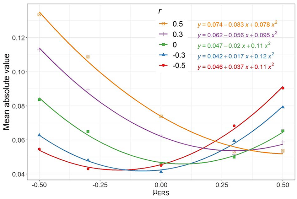
Note. N = test length; r = the content-ERS correlation; µ, μ_ERS, and $σ_{E R S}^{2}$ = the content mean, the ERS mean, and the ERS variance in sample B, respectively; △R² = the change in R².

Figure 2 demonstrates the interaction between the content-ERS correlation and the ERS difference_. It displays the MAB when N = 5, μ = .5, and μ²_ERS = .5. When the ERS difference was −.5, MAB increased from .055 to .133 as the content-ERS correlation increased from −.5 to .5. On the contrary, when and the ERS difference was .5, MAB decreased from .090 to .054 as the content-ERS correlation increased from −.5 to .5. Figure 2 also displays the fitted lines and equations of regressing MAB on the ERS difference and its quadratic form under each level of content-ERS correlations. As the content-ERS correlation increased from −.5 to .5, the coefficient of the ERS difference declined .120 from .037 to −.083.

Figure 2.

The MAB of the content difference estimate in MNRM-GPCM when N = 5, k = 4, µ = .5, and $σ_{E R S}^{2}$ = .5.

Figure 3 uses sample B’s response distributions to demonstrate the quadratic effect of the ERS difference on MAB. It displays the response distributions when μ_ERS = −.5, 0, and .5, given N = 5, r = 0, µ = .5, and σ²_ERS = .5. We did not present sample A’s response distributions because sample A’s ERS mean was fixed to zero. The ERS difference denoted sample B’s ERS mean and did not influence Sample A’s response distributions. When the data was free of ERS, sample B’s responses were mainly at categories 3 and 4 because their content mean was .5. When sample B’s ERS was at a low level (µ_ERS = −.5), their extreme responses decreased greatly, and their middle responses increased greatly. By contrast, when sample B’s ERS increased to the median level (µ_ERS = 0), their responses distributions became close to the response distribution when no ERS. However, as sample B’s ERS increased to a high level (µ_ERS = .5), their middle responses decreased, and their extreme responses increased. This explained why the MAB in Figure 2 was smaller when µ_ERS = 0 than when µ_ERS = −.5 and .5, given r = 0.

Figure 3.

Sample B’s response distributions when N = 5, r = −.5, μ = .5, $σ_{E R S}^{2}$ = .5, and μ_ERS = −.5 and .5.

Empirical Example

We analyzed an empirical dataset from PISA 2012 (OECD, 2014) to check the effect of ERS on the content difference estimate in real data. We compared Austrian, China-Shanghai, and German students’ mathematics self-efficacy. We selected these samples because De Jong et al. (2008) found that Austrian students’ ERS level was higher than China-Shanghai students and close to German students. There were three forms of the PISA 2012 Student Questionnaire because of the rotation design in the student questionnaire (OECD, 2014). Only two forms contained the Mathematics Self-Efficacy Scale, and thus, we only included students who responded to these forms. Besides, students who responded less than half the items on the scale were discarded. Finally, the Austrian sample contained 3,111 students, with 49.9% being female and a mean age of 15.80 (SD = 0.29). The China-Shanghai sample contained 3,436 students, with 50.6% being female and a mean age of 15.80 (SD = 0.29). The German sample contained 2,801 students, with 49.7% being female and a mean age of 15.80 (SD = 0.29).

The Mathematics Self-Efficacy Scale contained eight items rated on a 4-point scale, with 1 = strongly agree, 2 = agree, 3 = disagree, and 4 = strongly disagree. The coefficient α was .85, .82, .92, and .81 in the whole sample, the Austrian sample, the China-Shanghai sample, and the German sample, respectively. The MNRM and the GPCM were used to fit the data, and the results were regarded as controlling ERS and without controlling ERS, respectively. The Austria sample was used as the reference group. Its means in mathematics self-efficacy and ERS were set at zero, and its variances in in mathematics self-efficacy and ERS were set at one. The other samples’ means and variances were freely estimated. Item parameters were constrained to be equal across groups so that the means were comparable. The analyses were conducted with the mirt package. Note that students in the data had different sampling probabilities. We used the sampling weights (final student weights in the dataset) to adjust for different sampling probabilities so that results could represent the population (cf. Rutkowski et al., 2010). The data were multilevel, that is, students were nested in schools, which were nested in countries. We acknowledge that it is a limitation that the MNRM and GPCM did not account for the multilevel character.

Table 3 displays the goodness-of-fit indices. The MNRM fitted the data better than the GPCM in all indices, and the likelihood ratio test also indicated that the MNRM had a better model fit (χ² = 232,708, df = 13, p < .001). In the MNRM, the correlation between ERS and mathematics self-efficacy was −.27 (SE = 0.01, p < .001). The ERS variances were .58 (SE = 0.01) in the German sample and 3.89 (SE = 0.06) in the China-Shanghai sample. Table 4 displays the mean estimates. China-Shanghai students showed much lower ERS than Austrian students (mean difference = −1.25, Cohen’s d = −0.81, p < .001). German students showed higher ERS than the Austrian students, but the difference was small (mean difference = 0.10, Cohen’s d = 0.11, p < .001). The results were consistent with previous research (De Jong et al., 2008).

Table 3.

The Goodness-of-Fit Indices of the MNRM and the GPCM in Responses to the Mathematics Self-Efficacy Scale.

	AIC	BIC	−2 × log likelihood	χ²	df	p-Value
GPCM	8,170,012	8,170,415	8,169,940	232,708	13	0
MNRM	7,937,333	7,937,904	7,937,232	232,708	13	0

Note: GPCM = the generalized partial credit model; MNRM = the multidimensional nominal response model; AIC = Akaike’s information criterion; BIC = Bayesian information criterion.

Table 4.

The Means of ERS and Mathematics Self-Efficacy.

Country (sample size)	M (SE)
	Mathematics self-efficacy		ERS
	Controlling ERS	Without controlling ERS	ERS
Austria (3,111)	0 (−)	0 (−)	0 (−)
China-Shanghai (3,436)	2.22 (0.02)***	1.24 (0.01)***	−1.25 (0.02)***
German (2,801)	0.17 (0.01)***	0.31 (0.01)***	0.10 (0.01)***

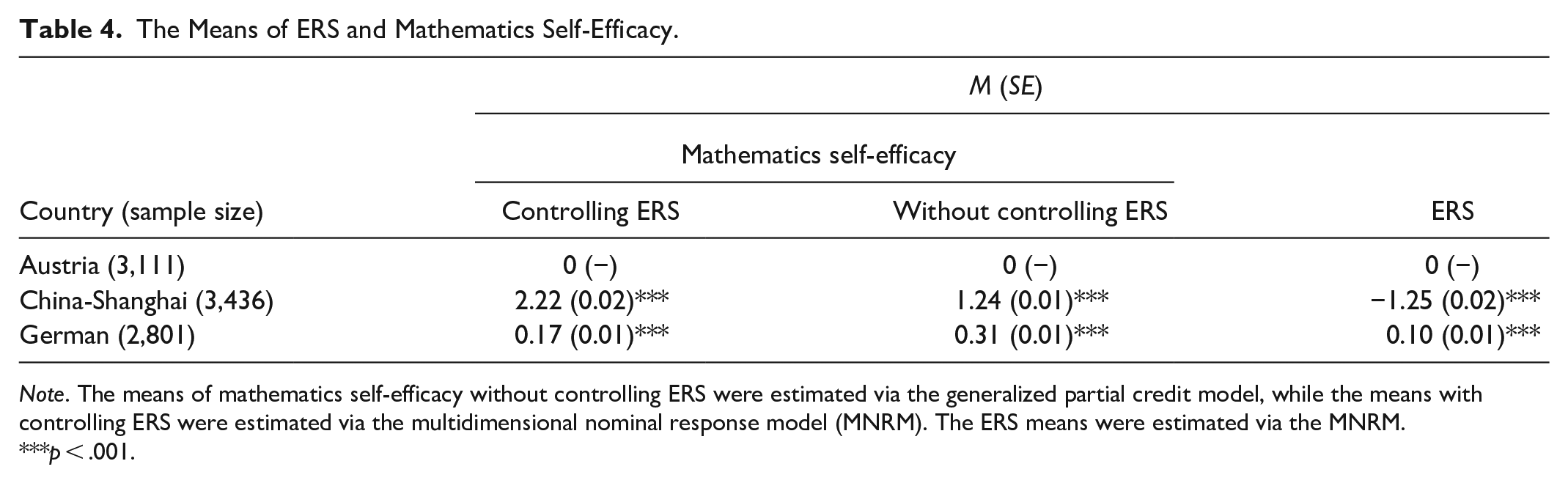
Note. The means of mathematics self-efficacy without controlling ERS were estimated via the generalized partial credit model, while the means with controlling ERS were estimated via the multidimensional nominal response model (MNRM). The ERS means were estimated via the MNRM.

***

p < .001.

The estimates of the mathematics self-efficacy differences between German and Austrian students were almost the same under the condition of controlling ERS (mean difference = 0.31, Cohen’s d = 0.31, p < .001) and without controlling ERS (mean difference = 0.17, Cohen’s d = 0.18, p < .001). Given that the MNRM fitted the data better than the GPCM, the two close estimates suggest that without controlling ERS might only cause a small bias in the estimate of the mathematics self-efficacy differences between German and Austrian students. The estimates of the mathematics self-efficacy difference between China-Shanghai and Austrian students differed greatly under the condition of controlling ERS (mean difference = 2.22, Cohen’s d = 1.66, p < .001) and without controlling ERS (mean difference = 1.24, Cohen’s d = 0.99, p < .001). The large difference between the two estimates suggests that without controlling ERS might cause a substantial bias in the estimate of the mathematics self-efficacy difference between China-Shanghai and Austrian students. These results were consistent with Figure 2, which showed that ERS caused greater biases when two groups had great ERS differences than when two groups had smaller ERS differences.

Study 2

Methods

Simulation design

The design of study 2 was nearly the same as that of study 1. The only difference was the levels of μ and the number of replications. The levels of μ changed from 0, .3, .5 to 0, .1, .2, .3 since pilot simulations revealed that the impact of ERS on the result of the independent t-test disappeared when μ reached .3 (see Figure 7). Simulations under the condition of μ > .3 could not generate more information about the impact of ERS than under the condition of µ = .3. The other settings were the same as study 1. The MNRM was used again to generate data with ERS contamination, while the GPCM was used to generate data without ERS contamination. Since study 2 did not entail model estimation, we increased the number of replications to 10,000 per condition.

Analyses

Study 2 focused on the mean comparison with manifest variables, so a scale score (the average across items) was computed as the manifest variable, and the independent t-test was conducted to compare the scale score between sample A and sample B. The null hypothesis assumed that there was no difference. Based on the p-value in the result of the t-test and the value of true group difference (i.e., μ), the results can be classified into four possible categories: true positives (the null hypothesis is true and not rejected, i.e., μ = 0 and p ≥ .05.), type I error (the null hypothesis is true but rejected, i.e., μ = 0 but p < .05.), type II error (the null hypothesis is false but not rejected, i.e., μ > 0 but p ≥ .05.), and true negatives (the null hypothesis is false and rejected, i.e., μ > 0 and p < .05.). When μ = 0, the type I error rate ([the count of type I error]/10,000) in every condition was computed to indicate the probability that the null hypothesis is true but rejected at .05 significance level. When μ > 0, the type II error rate ([the count of type II error]/10,000) was computed in every condition to indicate the probability that the null hypothesis is false but not rejected at .05 significance level. Comparing type I and II error rates between the data with and without ERS contamination will help understanding the specific impact of ERS on the result of the t-test.

Results

Type I error

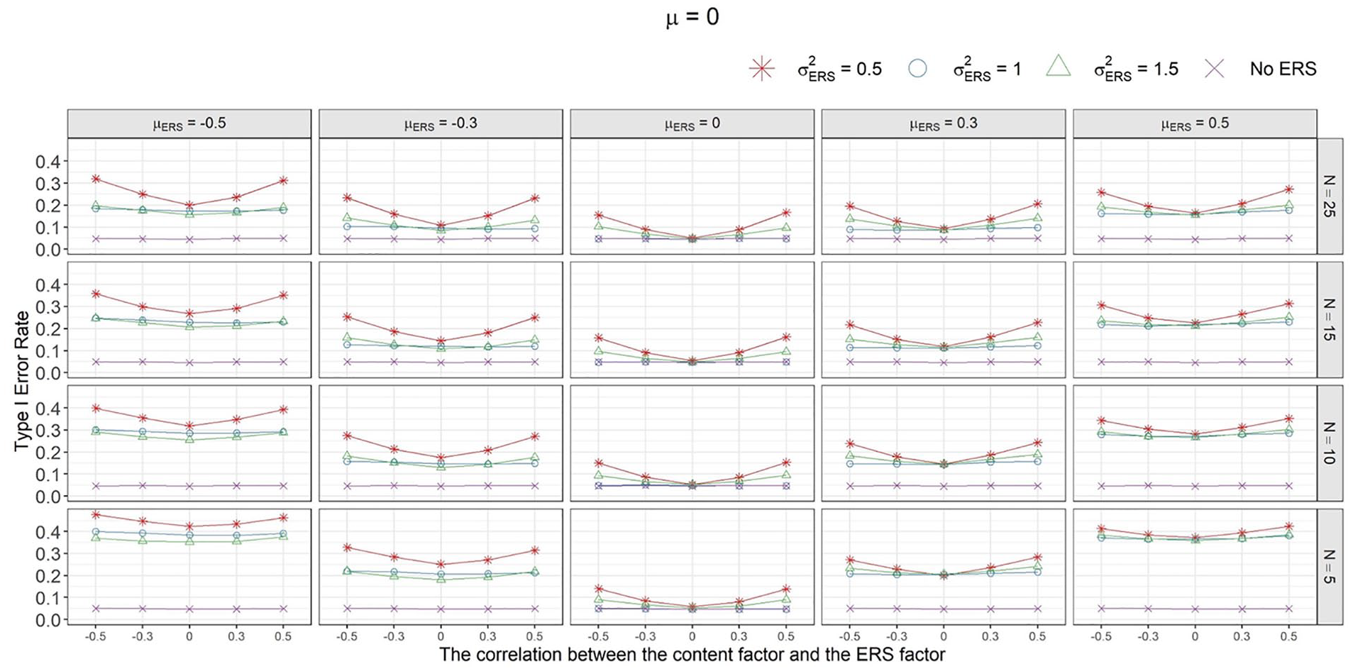
Figure 4 shows type I error rates under various conditions. Overall, when ERS contaminated the data, the type I error rate was higher than the benchmark (the type I error rate when the data were free from ERS). Like study 1, the ERS difference (µ_ERS) had a quadratic effect on the type I error rate. Taking the type I error rates when N = 5, r = 0, $σ_{E R S}^{2}$ = .5 as an example (the third red stars of each plot in the bottom row of Figure 4). As the ERS difference increased from −.5 to 0, the type I error rate declined from .42 to .06. However, as the ERS difference continued to increase from 0 to .5, the type I error rate went up to .37.

Figure 4.

The type I error rate when μ = 0.

Sample B’s ERS variance ( $σ_{E R S}^{2}$ ) also moderated the impact of ERS, especially when it was .5. Within a plot, the red stars were above the other points. Moreover, there was an interaction between sample B’s ERS variance and the content-ERS correlation. Within a plot, as the content-ERS correlation increased from −.5 to 0, the type I error rate when $σ_{E R S}^{2}$ = .5 firstly went down and then went up, but the error rate changed little when $σ_{E R S}^{2}$ = 1 or 1.5. Sample B’s ERS variance also interacted with the ERS difference. For instance, in the first row of Figure 4, given r = −.5 and μ_ERS = −.5, the type I error rate difference was .12 between the conditions that sample B’s ERS variances were .5 and 1.5. In contrast, given r = −.5 and µ_ERS = 0, the difference decreased to .05.

Besides, test length mitigated the undesirable impact of ERS. For example, when µ_ERS = −.5, r = 0, $σ_{E R S}^{2}$ = .5 (the third red stars of each plot in the first column of Figure 4), as test length increased from 5 to 25, the type I error rate declined from .42 to .20.

Type II error

Figures 5 to 7 displays the type II error rate when µ = .1, .2, and .3, respectively. When µ = .1, the type II error rate in the data with ERS was higher than the benchmark. When µ = .2, the impact of ERS on the type II error rate was small, as indicated by the points overlapping. When µ = .3, the impact of ERS on the type II error rate disappeared (Figure 7).

Figure 5.

The type II error rate when μ = .1.

Figure 6.

The type II error rate when μ = .2.

Figure 7.

The type II error rate when μ = .3.

The moderation effect of the other variables on the impact of ERS mainly existed under the condition of µ = .1 (Figure 5). The effects of the ERS difference and test length on the type II error rate were the same as their effects on the type I error rate. The type II error rate in the data with ERS rose as the absolute value of the ERS difference increased and test length decreased. The effects of sample B’s ERS variance and its interaction with the content-ERS correlation on the type II error rate were different from their effects on the type I error rate. When sample B’s ERS variance was .5, the type II error rate increased monotonously and quickly as the content-ERS correlation increased. When sample B’s ERS variance was 1, the type II error rate also increased as the content-ERS correlation increased, but the effect was small. When sample B’s ERS variance was 1.5, the type II error rate decreased monotonously as the content-ERS correlation increased. Taking the first plot in the first row of Figure 5 as an example, as the content-ERS correlation increased from −.5 to .5, the type II error rate increased from .05 to .41 when sample B’s ERS variance was .5. However, when sample B’s ERS variance was 1.5, the type II error rate declined from .25 to .08. When sample B’s ERS variance was 1, the type II error rate only experienced a small change, increasing from .13 to .20, as the content-ERS correlation increased from −.5 to .5.

Figure 8 helps in understanding how ERS inflated the type II error rate and the interaction between sample B’s ERS variance and the content-ERS correlation. It shows the response distributions when µ = .1, µ_ERS = −.5, N = 5, which corresponds to the first plot in the bottom row of Figure 5. We first focused on how ERS inflated the type II error rate. The first column showed the response distribution when the content-ERS correlation was −.5. Compared with the data without ERS (green bars), when ERS existed in the data, sample A’s and B’s responses at category 4 were pulled toward middle categories. Sample A’s responses at category 1 were also pulled toward middle categories, but sample B’s responses were pushed toward category 1. This difference in responses at category 1 between samples A and B reduced their difference in the scale scores, which is why ERS caused higher type II error rates (recall sample B’s true content mean was larger than sample A). When the content-ERS correlation was .5 (the second column of Figure 8), sample A’s and B’s extreme responses were pulled toward middle categories to the same extent. However, more of sample A’s responses at category 1 was pulled toward middle categories than sample B. Thus, their difference in scale scores decreased. Consequently, ERS caused higher type II error rates.

Figure 8.

The response distributions when N = 5, μ = .1, and μ_ERS = −.5.

Next, we focused on the interaction between sample B’s ERS variance and the content-ERS correlation. When the content-ERS correlation was −.5, as sample B’s ERS variance increased from .5 to 1.5, the proportion of responses at category 1 increased, and the proportion of responses at category 2 decreased (the bottom left plot of Figure 8). This change in response distributions meant that, as sample B’s ERS variance increased from .5 to 1.5, their scales scores decreased, and thus, their difference with sample A in scale scores would decrease. Consequently, the type II error rates increased. In contrast, when the content-ERS correlation was .5, as sample B’s ERS variance rose from .5 to 1.5, the proportion of responses at category 3 decreased, and the proportion of responses at category 4 increased (the bottom right plot of Figure 8). As such, sample B’s scale scores increased, and their difference with sample A increased. Consequently, the type II error rates decreased as sample B’s variance rose from .5 to 1.5.

Discussion

There is an increasing interest in response styles, among which ERS is a common form (Bolt, 2015). ERS may cause biased results in mean comparisons (Moors, 2004, 2012). The current research systematically investigated the impact of ERS on the result of mean comparisons via two simulation studies. The results of study 1 indicated that ERS could cause biased estimates of the content difference between two groups, and an empirical study further illustrated the result. Study 2 found that ERS could inflate the rates of both type I and II errors. A set of factors moderated the impact of ERS in studies 1 and 2.

Moderating Factors in the Influence of ERS

The most notable factor that moderated the impact of ERS is the ERS difference between groups. In general, no matter the direction of the ERS difference, the greater it was, the stronger effect ERS had on mean comparisons (see Figures 1 –5). Figure 3 demonstrates the quadratic effect of the ERS difference. If sample B’s ERS level were low, their responses would be pulled toward the middle categories. If sample B’s ERS level were median, their response distributions would be less influenced than when they had low ERS. If sample B’s ERS level were high, their responses would be pulled toward the extreme categories.

The linear effect of the content-ERS correlation was small, but its quadratic effect was stronger. Moreover, it had a substantial interaction effect with the ERS difference on the content difference estimate in study 1 (see Figure 2 and Table 2). It also had a substantial interaction effect with the unequal ERS variances on type I and II error rates in study 2 (see Figures 4 and 5). Plieninger (2016) found that the linear effects of the content-ERS correlation were weak on the estimates of coefficient α and the association between two content variables. However, the content-ERS correlation had a strong quadratic effect on the estimate of coefficient α. Besides, the interaction between two content-ERS correlations strongly impacted the association estimate between the two content variables. Putting Plieninger’s (2016) study and the current research together, the findings of the content-ERS correlation suggest that future research on the impact of ERS should consider the quadratic effect of the content-ERS correlation and its interactions with other factors. For instance, the simulation design needs to cover both positive and negative content-ERS correlations.

Adams et al. (2019) found that large variances in response style substantially reduced the precision of content estimates. The current research found that larger sample B’s ERS variance did not cause more bias in the content estimate (see the bottom plot of Figure 1). The different findings might be due to a set of factors. For instance, Adams et al.’s (2019) study focused on individuals’ content estimates, but the current research focused on the estimates of group content means. The MNRM in Adams et al.’s (2019) study was an exploratory model of response styles, while the MNRM in the current research was a confirmatory model because of using the scoring function. Nevertheless, this study did reveal that unequal ERS variance inflated type I and II error rates. Overall, these findings suggest that the variance of response style is an critical factor in the response style effect.

The bias caused by ERS on the content difference estimate increased as the true content difference increased, although the overall effect was weak. However, the true content difference had a marked impact on the type II error rate. When the true content difference was small (e.g., μ = .1 in Figure 5 is corresponding to Cohen’s d = 0.1), ERS significantly inflated the type II error rate and decreased the statistical power. Although the impact of ERS hardly existed when μ = .2 and disappeared when μ = .3, the results do not necessarily imply that that researchers can ignore ERS when the content difference is large. The size of each sample in the simulations was 3,000. When the sample size is much smaller, for example, 200 or 500, the impact of ERS may reoccur even in the condition of a large content difference. In addition, ERS resulted in more biases in the content difference estimates as the true content difference increased. Thus, no matter the magnitude of the true content difference, the influence of ERS on mean comparisons should not be ignored.

Test length buffered the impact of ERS weakly on the content difference estimate but effectively on type I and II error rates. The finding on test length was in line with prior research (Wetzel, Böhnke, et al., 2016), where the bias in content estimates caused by ERS decreased as test length increased. The reason for the moderation effect of test length might be that, as test length increased, individual extreme responses caused by one’s high ERS contributed less to their scale scores. So did individual middle responses caused by low ERS. Consequently, the t-test based on scale scores was less impacted by ERS as test length increased.

Implications

The large moderation effect of the ERS difference on the influence of ERS implies if evidence indicates that the groups of interest have substantial ERS differences, researchers need to control ERS. Otherwise, the difference estimate and the results of statistical tests would be untrustworthy. For instance, previous studies indicated that ERS is positively related to education levels and Hofstede’s cultural dimensions (individualism, uncertainty avoidance, masculinity, and power distance; see De Jong et al., 2008; Hofstede, 2005; Johnson et al., 2005). Thus, if the groups used for mean comparisons differed substantially in education and the cultural dimensions, the effect of ERS may be large and need to be controlled.

On the other hand, even if the groups of interest have no difference in ERS, researchers should still not ignore ERS. The other factors considered in this study, including true content differences, content-ERS correlation, unequal ERS variances, and test length, also moderated the impact of ERS on mean comparisons, and these factors interacted with each other in the impact of ERS. When there was a high content-ERS correlation, unequal ERS variances, or few items, the influence of ERS was nontrivial, no matter the size of ERS differences. The only case that researchers can safely ignore ERS may be that there is no ERS difference and no content-ERS correlation. It may be challenging to prove that these rigorous prerequisites are met in empirical studies. Thus, we recommend researchers control ERS in mean comparisons as possible as they can.

In particular, cross-country studies based on data from international large-scale surveys should control ERS. In the empirical example of this study, which used the PISA 2012 data, the estimate of mathematics self-efficacy difference between Austrian and China-Shanghai changed substantially after modeling ERS. This is in line with Khorramdel et al.’s (2019) study, which also analyzed PISA 2012 data and found that the correlations between personality scales and cognitive skills became more meaningful after correcting ERS and the midpoint response style. Khorramdel et al.’s study and the empirical example of this study call for correcting response style effects when making comparisons in country-level measures derived from international large-scale surveys.

The main method to control ERS is modeling it during data analysis, such as the MNRM used in the current research. However, models like MNRM are complex. Researchers may lack the necessary knowledge to apply these statistical methods to control ERS. Besides, modeling ERS after data collection may reduce stakeholders’ trust in the results because explaining the rationale and procedure of modeling ERS to them is challenging. In such cases, controlling ERS during tool design and data collection is a better option. Results in this study suggest increasing test length to mitigate the impact of ERS, but 15 items for a single construct may be sufficient because the impact of ERS weakened slightly when test length increased from 15 to 25 (see Figures 1, 4, and 5). Other characteristics of rating scale also reduce the presence of ERS, such as the number of response categories (Weijters et al., 2010a) and response format (Böckenholt, 2017). The data collection approach is also a critical factor. For instance, a face-to-face survey may trigger more extreme responses than a web survey (Liu et al., 2017).

There were contrary results in existing empirical studies about the impact of ERS on mean comparisons. For instance, Moors (2004) found that the group difference became significantly smaller when ERS was taken into account in data analyses, while He and Van de Vijver’s (2015) study, the group difference hardly changed after controlling ERS. The results in the current study might help us explain the contrary findings. Although test length was close in Moors’ (2004) as well as He and Van de Vijver’s (2015) studies, the ERS difference, content-ERS correlation, and unequal ERS variances might differ between the two studies given that they did not use the same sample. In Moors’s (2004) study, there might be a substantial ERS difference and content-ERS correlation, so ERS had a considerable impact on the result of mean comparisons. On the contrary, there might be no ERS difference and content-ERS correlation in He and Van de Vijver’s (2015) study. In this case, ERS would not influence the result of mean comparisons. In summary, further research on the impact of response styles should consider the moderation of multiple factors. Whether a response style influences the results of data analysis cannot be concluded based on a single dataset.

Limitations and Future Directions

This study focused on mean comparison in one variable between two independent groups. Other conditions, such as dependent groups, multiple groups, and multiple variables, are not covered herein and remain to be investigated. Whether ERS influences the type I and II errors rates in non-parametric tests is also an interesting topic. If ERS has weak effects in non-parametric tests, these tests may be used as an approach to control ERS, given that the current statistical models of ERS, such as MNRM in this study, are complex. It is challenging for researchers not familiar with these models to apply them to control ERS in practice. There are simpler methods for controlling ERS, such as the regression residual technique, which regresses the raw scale scores on ERS and uses the residuals as new scale scores (Baumgartner et al., 2001). However, the effectiveness of these methods may be less satisfactory than the complex models (Wetzel, Böhnke, et al., 2016; Zhang & Wang, 2020). Further studies need to develop a relatively simple yet effective approach.

ERS in this study refers to the tendency to select extreme options. Although this definition is used widely, some researchers may prefer a different definition, such as the tendency to select more extreme options (Jin & Wang, 2014; Tutz & Berger, 2016). The current results may not generalize to other ERS definitions. How ERS under other definitions influences mean comparison entails further research.

The current research did not cover response styles other than ERS, such as the middle point response style (the tendency to select middle categories) and the acquiescence response style (the tendency to select categories stating agreement; Van Vaerenbergh & Thomas, 2013). It would be interesting to investigate how these response styles influence the results of mean comparisons. Moreover, different response styles may exist in the same data (Wetzel & Carstensen, 2017). It is possible that different response styles interact with each other in the impact on mean comparisons.

The sizes of content difference, ERS difference, and unequal ERS variances in the simulations were smaller than the empirical example. For instance, the maximum ERS difference was .5 in simulations, while the ERS difference between Austrian and China-Shanghai samples was 1.25. Given that the effect of ERS strengthened as these factors became bigger, the ERS effect in simulations may be smaller than in empirical data. Indeed, the content difference estimate between Austrian and China-Shanghai samples increased .98 after controlling ERS, while the maximum bias in the simulation of study 1 was .133. Thus, researchers should keep in mind that the effect of ERS can be much larger in the real world than what the simulations showed.

Conclusion

This simulation research systematically investigated the bias that ERS caused in content difference estimates and type I and II error rates in independent t-tests. ERS differences and their interaction with the content-ERS correlation increased the bias in content difference estimates. ERS differences, short tests, and unequal ERS variances inflated the type I and II error rates. Besides, the interaction between unequal ERS variances and content-ERS correlations strongly impacted type I and II error rates. Future research on the ERS effect should consider the ERS variance and content-ERS correlations. Given that the undesirable effect of ERS depended on various factors and their interactions, it may be challenging to prove that ERS can be ignored in a particular empirical dataset. Thus, empirical research should account for ERS in mean comparisons, no matter the mean comparisons are based on latent or manifest variables.

Footnotes

Appendix

Table A4.

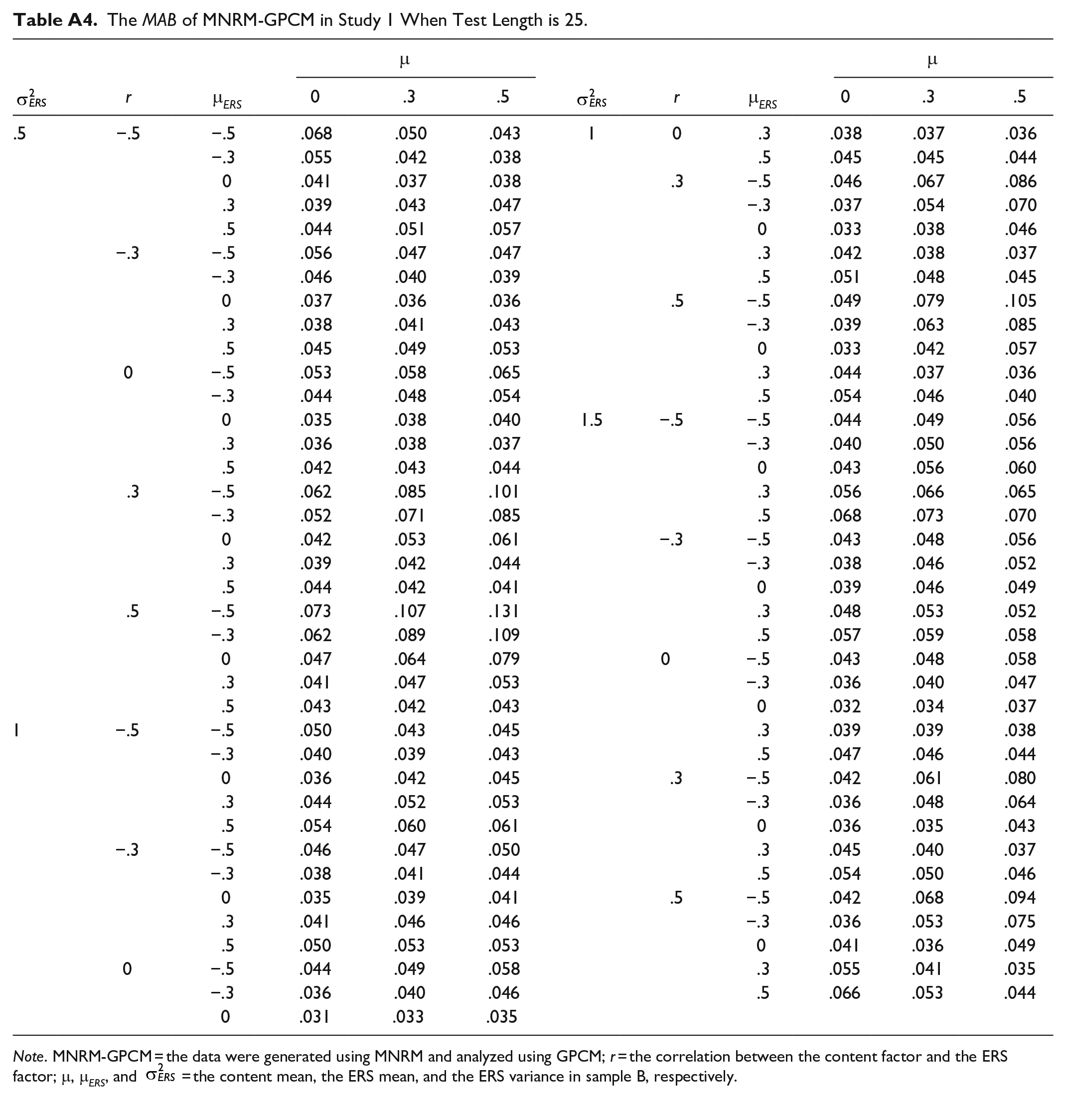
The MAB of MNRM-GPCM in Study 1 When Test Length is 25.

$σ_{E R S}^{2}$	r	μ _ERS	μ			$σ_{E R S}^{2}$	r	μ _ERS	μ
$σ_{E R S}^{2}$	r	μ _ERS	0	.3	.5	$σ_{E R S}^{2}$	r	μ _ERS	0	.3	.5
.5	−.5	−.5	.068	.050	.043	1	0	.3	.038	.037	.036
		−.3	.055	.042	.038		0	.5	.045	.045	.044
		0	.041	.037	.038		.3	−.5	.046	.067	.086
		.3	.039	.043	.047			−.3	.037	.054	.070
		.5	.044	.051	.057			0	.033	.038	.046
	−.3	−.5	.056	.047	.047			.3	.042	.038	.037
		−.3	.046	.040	.039			.5	.051	.048	.045
		0	.037	.036	.036		.5	−.5	.049	.079	.105
		.3	.038	.041	.043			−.3	.039	.063	.085
		.5	.045	.049	.053			0	.033	.042	.057
	0	−.5	.053	.058	.065			.3	.044	.037	.036
		−.3	.044	.048	.054			.5	.054	.046	.040
		0	.035	.038	.040	1.5	−.5	−.5	.044	.049	.056
		.3	.036	.038	.037			−.3	.040	.050	.056
		.5	.042	.043	.044			0	.043	.056	.060
	.3	−.5	.062	.085	.101			.3	.056	.066	.065
		−.3	.052	.071	.085			.5	.068	.073	.070
		0	.042	.053	.061		−.3	−.5	.043	.048	.056
		.3	.039	.042	.044			−.3	.038	.046	.052
		.5	.044	.042	.041			0	.039	.046	.049
	.5	−.5	.073	.107	.131			.3	.048	.053	.052
		−.3	.062	.089	.109			.5	.057	.059	.058
		0	.047	.064	.079		0	−.5	.043	.048	.058
		.3	.041	.047	.053			−.3	.036	.040	.047
		.5	.043	.042	.043			0	.032	.034	.037
1	−.5	−.5	.050	.043	.045			.3	.039	.039	.038
		−.3	.040	.039	.043			.5	.047	.046	.044
		0	.036	.042	.045		.3	−.5	.042	.061	.080
		.3	.044	.052	.053			−.3	.036	.048	.064
		.5	.054	.060	.061			0	.036	.035	.043
	−.3	−.5	.046	.047	.050			.3	.045	.040	.037
		−.3	.038	.041	.044			.5	.054	.050	.046
		0	.035	.039	.041		.5	−.5	.042	.068	.094
		.3	.041	.046	.046			−.3	.036	.053	.075
		.5	.050	.053	.053			0	.041	.036	.049
	0	−.5	.044	.049	.058			.3	.055	.041	.035
		−.3	.036	.040	.046			.5	.066	.053	.044
		0	.031	.033	.035

Note. MNRM-GPCM = the data were generated using MNRM and analyzed using GPCM; r = the correlation between the content factor and the ERS factor; μ, μ_ERS, and $σ_{E R S}^{2}$ = the content mean, the ERS mean, and the ERS variance in sample B, respectively.

Declaration of Conflicting Interests

The author(s) declared no potential conflicts of interest with respect to the research, authorship, and/or publication of this article.

Funding

The author(s) disclosed receipt of the following financial support for the research, authorship, and/or publication of this article: The work was supported by the China Scholarship Council [Grant number 201806040180].

ORCID iDs

Yingbin Zhang

Yehui Wang

Notes

References

Adams

D. J.

Bolt

D. M.

Deng

Smith

S. S.

Baker

T. B.

(2019). Using multidimensional item response theory to evaluate how response styles impact measurement. British Journal of Mathematical and Statistical Psychology, 72(3), 466–485. http://doi.org/10.1111/bmsp.12169

Aichholzer

(2013). Intra-individual variation of extreme response style in mixed-mode panel studies. Social Science Research, 42(3), 957–970. https://doi.org/10.1016/j.ssresearch.2013.01.002

Baird

B. M.

Lucas

R. E.

Donnellan

M. B.

(2017). The role of response styles in the assessment of intraindividual personality variability. Journal of Research in Personality, 69, 170–179. https://doi.org/10.1016/j.jrp.2016.06.015

Baumgartner

Steenkamp

J. E. B. M.

(2001). Response style in marketing research: A cross-national investigation. Journal of Marketing Research, 38(2), 143–156. https://doi.org/10.1509/jmkr.38.2.143.18840

Benítez

Van de Vijver

F. J. R.

Padilla

(2016). Linking extreme response style to response processes: A cross-cultural mixed methods approach. International Journal of Psychology, 51(6), 464–473. https://doi.org/10.1002/ijop.12379

Bock

R. D.

(1972). Estimating item parameters and latent ability when responses are scored in two or more nominal categories. Psychometrika, 37(1), 29–51. https://doi.org/10.1007/BF02291411

Böckenholt

(2012). Modeling multiple response processes in judgment and choice. Psychological Methods, 17, 665–678. https://doi.org/10.1037/a0028111

Böckenholt

(2017). Measuring response styles in likert items. Psychological Methods, 22(1), 69–83.

Bolt

D. M.

(2015). Surveys: Extreme response. In Wright

J. D.

(Ed.), International encyclopedia of the social & behavioral sciences (2nd ed., pp. 758–763). Elsevier. https://doi.org/10.1016/B978-0-08-097086-8.44065-1

10.

Bolt

D. M.

Johnson

T. R.

(2009). Addressing score bias and differential item functioning due to individual differences in response style. Applied Psychological Measurement, 33(5), 335–352. https://doi.org/10.1177/0146621608329891

11.

Bolt

D. M.

Kim

J.-S.

(2014). Measurement and control of response styles using anchoring vignettes: A model-based approach. Psychological Methods, 19, 528–541. https://doi.org/10.1037/met0000016

12.

Bolt

D. M.

Newton

J. R.

(2011). Multiscale measurement of extreme response style. Educational and Psychological Measurement, 71(5), 814–833. http://doi.org/10.1177/0013164410388411

13.

Chalmers

R. P.

(2012). mirt: A multidimensional item response theory package for the R environment. Journal of Statistical Software, 48(6), 1–29. https://doi.org/10.18637/jss.v048.i06

14.

De Boeck

Partchev

(2012). IRTrees: Tree-based item response models of the GLMM family. Journal of Statistical Software, 48, 1–28. https://doi.org/10.18637/jss.v048.c01

15.

De Jong

M. G.

Steenkamp

J. B. E. M.

Fox

J. P.

Baumgartner

(2008). Using item response theory to measure extreme response style in marketing research: A global investigation. Journal of Marketing Research, 45(1), 104–115. https://doi.org/10.1509/jmkr.45.1.104

16.

Falk

C. F.

Cai

(2016). A flexible full-information approach to the modeling of response styles. Psychological Methods, 21(3), 328–347. https://doi.org/10.1037/met0000059

17.

Van de Vijver

F. J. R.

(2015). Effects of a general response style on cross-cultural comparisons evidence from the teaching and learning international survey. Public Opinion Quarterly, 79(S1), 267–290. https://doi.org/10.1093/poq/nfv006

18.

Van de Vijver

F. J. R.

(2016). Response styles in factual items: Personal, contextual and cultural correlates. International Journal of Psychology, 51(6), 445–452. https://doi.org/10.1002/ijop.12263

19.

Henninger

(2021). A novel partial credit extension using varying thresholds to account for response tendencies. Journal of Educational Measurement, 58(1), 104–129. https://doi.org/10.1111/jedm.12268

20.

Henninger

Meiser

(2020). Different approaches to modeling response styles in divide-by-total IRT models (Part I): A model integration. Psychological Methods, 25, 560–576. https://doi.org/10.1037/met0000249

21.

Hoffmann

Mai

Cristescu

(2013). Do culture-dependent response styles distort substantial relationships? International Business Review, 22(5), 814–827. http://doi.org/10.1016/j.ibusrev.2013.01.008

22.

Hofstede

G. J.

(2005). Cultures and organisations: Software of the mind (3rd ed.). McGraw-Hill.

23.

Jin

Wang

(2014). Generalized IRT models for extreme response style. Educational and Psychological Measurement, 74(1), 116–138. https://doi.org/10.1177/0013164413498876

24.

Johnson

Kulesa

Cho

Y. I.

Shavitt

(2005). The relation between culture and response styles evidence from 19 countries. Journal of Cross-Cultural Psychology, 36(2), 264–277. https://doi.org/10.1177/0022022104272905

25.

Khorramdel

Jeon

Wang

L. L.

(2019). Advances in modelling response styles and related phenomena. British Journal of Mathematical and Statistical Psychology, 72(3), 393–400. https://doi.org/10.1111/bmsp.12190

26.

Kieruj

N. D.

Moors

(2010). Variations in response style behavior by response scale format in attitude research. International Journal of Public Opinion Research, 22(3), 320–342. https://doi.org/10.1093/ijpor/edq001

27.

Kieruj

N. D.

Moors

(2013). Response style behavior: Question format dependent or personal style? Quality & Quantity, 47(1), 193–211. https://doi.org/10.1007/s11135-011-9511-4

28.

Leventhal

B. C.

(2019). Extreme response style: A simulation study comparison of three multidimensional item response models. Applied Psychological Measurement, 43(4), 322–335. https://doi.org/10.1177/0146621618789392

29.

Leventhal

B. C.

Stone

C. A.

(2018). Bayesian analysis of multidimensional item response theory models: A discussion and illustration of three response style models. Measurement: Interdisciplinary Research and Perspectives, 16(2), 114–128. https://doi.org/10.1080/15366367.2018.1437306

30.

Liu

Conrad

F. G.

Lee

(2017). Comparing acquiescent and extreme response styles in face-to-face and web surveys. Quality & Quantity, 51, 1–18.

31.

Bolt

D. M.

(2015). Examining the attitude-achievement paradox in PISA using a multilevel multidimensional IRT model for extreme response style. Large-scale Assessments in Education, 3(2), 1–18. https://doi.org/10.1186/s40536-015-0012-0

32.

Meisenberg

Williams

(2008). Are acquiescent and extreme response styles related to low intelligence and education? Personality and Individual Differences, 44(7), 1539–1550. https://doi.org/10.1016/j.paid.2008.01.010

33.

Moors

(2004). Facts and artefacts in the comparison of attitudes among ethnic minorities: A multigroup latent class structure model with adjustment for response style behavior. European Sociological Review, 20(4), 303–320. https://doi.org/10.1093/esr/jch026

34.

Moors

(2012). The effect of response style bias on the measurement of transformational, transactional, and laissez-faire leadership. European Journal of Work and Organizational Psychology, 21(2), 271–298. https://doi.org/10.1080/1359432X.2010.550680

35.

Mottus

Allik

Realo

Rossier

Zecca

Ah-Kion

Amoussou-Yeye

Backstrom

Barkauskiene

Barry

Bhowon

Bjorklund

Bochaver

de Bruin

Cabrera

H. F.

Chen

S. X.

Church

A. T.

Cisse

D. D.

, . . . Johnson

(2012). The effect of response style on self-reported Conscientiousness across 20 countries. Personality & Social Psychology Bulletin, 38(11), 1423–1436. https://doi.org/10.1177/0146167212451275

36.

Mullis

I. V. S.

Martin

M. O.

(2013). TIMSS 2015 assessment frameworks. TIMSS & PIRLS International Study Center and International Association for the Evaluation of Educational Achievement.

37.

Muraki

(1992). A generalized partial credit model: Application of an EM algorithm. Applied Psychological Measurement, 16(2), 159–176. https://doi.org/10.1002/j.2333-8504.1992.tb01436.x

38.

OECD. (2014). PISA 2012 technical report. OECD Publishing.

39.

Paulhus

D. L.

(1991). Measurement and control of response bias. In Robinson

J. P.

Shaver

P. R.

Wrightsman

L. S.

(Eds.), Measures of social psychological attitudes (pp. 17–59). Academic Press. https://doi.org/10.1016/B978-0-12-590241-0.50006-X

40.

Plieninger

(2016). Mountain or molehill? A simulation study on the impact of response styles. Educational and Psychological Measurement, 77(1), 32–53. https://doi.org/10.1177/0013164416636655

41.

Podsakoff

P. M.

MacKenzie

S. B.

Podsakoff

N. P.

(2012). Sources of method bias in social science research and recommendations on how to control it. Annual Review of Psychology, 63, 539–569. https://doi.org/10.1146/annurev-psych-120710-100452

42.

Rost

Carstensen

Von Davier

(1997). Applying the mixed Rasch model to personality questionnaires. In Rost

Langeheine

(Eds.), Applications of latent trait and latent class models in the social sciences (pp. 324–332). Waxmann Verlag.

43.

Rutkowski

Gonzalez

Joncas

Von Davier

(2010). International large-scale assessment data: Issues in secondary analysis and reporting. Educational Researcher, 39(2), 142–151. http://doi.org/10.3102/0013189X10363170

44.

Thissen

Steinberg

(1986). A taxonomy of item response models. Psychometrika, 51(4), 567–577. https://doi.org/10.1007/BF02295596

45.

Tutz

Berger

(2016). Response styles in rating scales simultaneous modeling of content-related effects and the tendency to middle or extreme categories. Journal of Educational and Behavioral Statistics, 41(3), 239–268. https://doi.org/10.3102/1076998616636850

46.

Van Vaerenbergh

Thomas

T. D.

(2013). Response styles in survey research: A literature review of antecedents, consequences, and remedies. International Journal of Public Opinion Research, 25(2), 195–217. https://doi.org/10.1093/ijpor/eds021

47.

Weijters

Geuens

Schillewaert

(2010a). The individual consistency of acquiescence and extreme response style in self-report questionnaires. Applied Psychological Measurement, 34(2), 105–121. https://doi.org/10.1177/0146621609338593

48.

Weijters

Geuens

Schillewaert

(2010b). The stability of individual response styles. Psychological Methods, 15(1), 96–110. https://doi.org/10.1037/a0018721

49.

Wetzel

Böhnke

J. R.

Rose

(2016). A simulation study on methods of correcting for the effects of extreme response style. Educational and Psychological Measurement, 76(2), 304–324. https://doi.org/10.1177/0013164415591848

50.

Wetzel

Carstensen

C. H.

(2017). Multidimensional modeling of traits and response styles. European Journal of Psychological Assessment, 33(5), 352–364. https://doi.org/10.1027/1015-5759/a000291

51.

Wetzel

Carstensen

C. H.

Böhnke

J. R.

(2013). Consistency of extreme response style and non-extreme response style across traits. Journal of Research in Personality, 47(2), 178–189. https://doi.org/10.1016/j.jrp.2012.10.010

52.

Wetzel

Lüdtke

Zettler

Böhnke

J. R.

(2016). The stability of extreme response style and acquiescence over 8 years. Assessment, 23(3), 279–291. https://doi.org/10.1177/1073191115583714

53.

Yuan

Bentler

P. M.

(2006). Mean comparison: Manifest variable versus latent variable. Psychometrika, 71(1), 139.

54.

Zhang

Wang

(2020). Validity of three IRT models for measuring and controlling extreme and midpoint response styles. Frontiers in Psychology, 11, 271. https://doi.org/10.3389/fpsyg.2020.00271

The Impact of Extreme Response Style on the Mean Comparison of Two Independent Samples

Abstract

Keywords

Introduction

Extreme Response Style (ERS)

Multidimensional Nominal Response Model (MNRM) for Extreme Response Style

The Current Study

Study 1

Methods

Simulation design

Analyses

Results

Empirical Example

Study 2

Methods

Simulation design

Analyses

Results

Type I error

Type II error

Discussion

Moderating Factors in the Influence of ERS

Implications

Limitations and Future Directions

Conclusion

Footnotes

Appendix

Declaration of Conflicting Interests

Funding

ORCID iDs

Notes

References