Sage Journals: Discover world-class research

Abstract

This article investigates the profitability of candlestick patterns. The holding periods are 1, 3, 5, and 10 days. Two exit strategies are studied. One is the Marshall–Young–Rose (MYR) exit strategy and the other is the Caginalp–Laurent (CL) exit strategy. The MYR applies a prespecified date to exit the market. In contrast, the CL sets an exit price equal to an average holding period closing price, assuming that investors liquidate their positions evenly within this period. The daily data include open, high, low, and close prices of component stocks of the SET50 index (the 50 largest capitalization stocks in the Stock Exchange of Thailand [SET]) for a 10-year period from July 3, 2006, to June 30, 2016. This study tests the predictive power of bullish and bearish candlestick reversal patterns both without technical filtering and with technical filtering (Stochastics [%D], Relative Strength Index [RSI], Money Flow Index [MFI]) by applying the skewness adjusted t test and the binomial test. The statistical analysis finds little use of both bullish and bearish candlestick reversal patterns since the mean returns of most patterns are not statistically different from zero. Even the ones with statistically significant returns do have high risks in terms of standard deviations. The binomial test results also indicate that candlestick patterns cannot reliably predict market directions. In addition, this article finds that filtering by %D, RSI, or MFI generally does not increase profitability nor prediction accuracy of candlestick patterns.

Keywords

technical analysis trading rule candlestick charting pattern

Introduction

The candlestick chart was first developed in Japan and then became popular around the world after its introduction to the West by Nison (1991). It is very common for investors to use them in conjunction with other technical indicators. In fact, according to a survey by Menkhoff (2010), fund managers apply it in their shorter term forecasts. Candlestick charting is unique in the sense that it concurrently plots daily open, high, low, and close price movements (Morris, 2006). As such, it reveals demand and supply changing balance (Caginalp & Laurent, 1998) and also investor sentiment and psychology (Marshall, Young, & Rose, 2006). Proponents of candlestick believe that investors could use these chart patterns to predict short-term price movements or future turning points.

Surprisingly, despite its long history and popularity, there are not many academic studies on candlestick patterns. There is still no agreement whether this approach is profitable. Some studies find that it is useless (Horton, 2009; Marshall, Young, & Cahan, 2008; Marshall, Young, & Rose, 2007) at least in the U.S. and Japanese stock markets. However, other studies find that applying certain candlestick patterns is profitable at least for short-term trading (Goo, Chen, & Chang, 2007; Lu & Shiu, 2012; Lu, Shiu, & Liu, 2012; Shiu & Lu, 2011; Zhu, Atri, & Yegen, 2016), at least in the Taiwanese and Chinese stock markets. Interestingly, Lu, Chen, and Hsu (2015) even find significant positive returns in the U.S. stock markets if investors follow the Caginalp–Laurent (CL) exit strategies (Caginalp & Laurent, 1998) but not the Marshall–Young–Rose (MYR) exit strategies (Marshall et al., 2006). The MYR applies a prespecified date to exit the market, whereas the CL sets an exit price equal to an average holding period closing price.

This article tests the profitability of candlestick trading strategies both without technical filtering and with technical filtering by applying the skewness adjusted t test (Johnson, 1978) and the binomial test. The data cover daily open, high, low, and close prices of component stocks of the SET50 index for a 10-year period from July 3, 2006, to June 30, 2016. The study on an individual stock data set has an advantage over a study on a stock index in a sense that each stock is tradable unlike a nontradable stock index. Moreover, the use of individual stock data avoids potential biases introduced by nonsynchronous trading within an index.

As previous literature focuses on the mature markets of the United States and Japan and the emerging markets of only Taiwan and China, this article extends the literature to include the Southeast Asian emerging market of Thailand. Moreover, the article investigates further the impact of different exit strategies. This important issue has not been investigated outside the U.S. market or after Lu et al. (2015). In addition, the use of Thai stock data to test candlestick patterns, which were developed using Japanese rice data and formerly tested only in the U.S., Japanese, and Chinese stock markets, is clearly an ex ante evaluation. This mitigates the issue of data snooping (Marshall et al., 2006). In addition, this study also tests profitability of filtered candlestick patterns, which is the use of candlesticks in combination with other technical indicators. The applied technical filters are Stochastics (%D), Relative Strength Index (RSI), and Money Flow Index (MFI). Basically, the buy or sell signals must be confirmed by other indicators before they are acted upon to avoid false signals. This test has not been done in previous studies which focus exclusively on candlestick patterns.

The empirical results reveal that most candlestick reversal patterns do not generate statistically significant mean returns. Moreover, even some patterns that do have significant mean returns usually have very high risks in terms of standard deviations. The binomial tests also confirm that most candlestick patterns, even the ones with significant mean returns, cannot reliably predict market directions. In addition, this article finds that filtering either by %D, RSI, or MFI generally does not increase profitability nor prediction accuracy of candlestick patterns.

The organization of this article is as follows. The “Introduction” section provides a brief summary. “Literature Review” section discusses both theories and existing empirical evidences. “Candlestick Methodology” section provides a background of candlestick methodology. “Method” section discusses the statistical method. The “Data” section provides a discussion about data. “Empirical Results” and “Filtered Candlestick Patterns” sections provide empirical results without technical filtering and with technical filtering, respectively. Finally, the “Conclusion” section concludes and suggets further studies.

Literature Review

Theory

The Efficient Market Hypothesis (EMH) states that security prices already reflect all available and relevant information (Fama, 1970). As a result, technical analysis including charting patterns, which use only historical trading data, cannot generate positive abnormal returns. Investors could make money from charting patterns only if the market is inefficient.

However, later theories start to challenge the EMH. Grossman and Stiglitz (1980) theoretically demonstrate that, if the market is perfectly efficient, then there is no benefits in obtaining and analyzing costly information. The question is then how could security prices reflect information when no one is willing to process it. Therefore, the market cannot be perfectly efficient. More recently, behavioral models, such as noisy rational expectations models (Brown & Jennings, 1989), feedback models (DeLong, Shleifer, & Summers, 1990), and herding models (Froot, Scharftstein, & Stein, 1992) challenge the EMH. These models argue that price adjusts slowly to new information due to noise, feedback mechanism, or herding behavior. In these models, it is possible for trading strategies based on past data to generate positive abnormal returns. As such, charting patterns may still be useful for profitable trading.

Empirical Studies

The earliest test of candlestick trading strategies is Caginalp and Laurent (1998). They used daily prices of all S&P500 stocks over the 1992-1996 period to test the prediction accuracy of candlestick patterns. Their binomial tests, as approximated by the normal distribution, indicate statistical significance and an almost 1% return over a 2-day horizon. However, later work by Marshall et al. (2006) and Marshall et al. (2007) found the opposite conclusion. Their results could not find profits from the use of candlestick patterns onDow Jones Industrial Average (DJIA) stocks over the 1992-2002 period. Their method is an extension of the bootstrapping methodology that accommodates open, high, low, and close prices. They conclude that the candlestick patterns have no forecasting power. Results are based on the assumption that a trade is executed at a close price on the day after a signal. Stocks are generally held for up to 10 days. Horton (2009) confirms these results. His article finds little value in the use of candlestick.

Unlike previous studies which focus on daily data, Duvinage, Mazza, and Petitjean (2013) test 5-min intraday data of 30 component stocks of the DJIA index. After a correction for the data snooping bias, no single candlestick rule on the double-or-out market timing strategy outperforms the buy-and-hold strategy after transaction costs.

Following Marshall et al. (2006), Marshall, Young, and Cahan (2008) used a similar approach in analyzing the largest 100 stocks listed on the Tokyo Stock Exchange. Their results show that candlestick charting could not generate positive abnormal returns in the Japanese equity market during 1975-2004. In fact, it is not even consistently profitable before transaction costs.

Lu et al. (2015) are later able to reconcile the conflicting results from Caginalp and Laurent (1998) and Marshall et al. (2006) by investigating profitability of two different exit strategies. The first one is the CL exit strategy (Caginalp & Laurent, 1998) and the other one is the MYR exit strategy (Marshall et al., 2006). The MYR applies a prespecified date to exit the market. On the contrary, the CL sets an exit price equal to an average holding period closing price, assuming that investors liquidate their positions evenly within this period. They apply candlestick trading strategies to the 30 component stocks of the DJIA index over the 1992-2012 period and find that candlestick patterns with the CL exit strategy are profitable even after transaction costs and corrections of data snooping bias. In sharp contrast, candlestick patterns with the MYR exit strategy are not profitable. They reason that positive abnormal returns of the CL exit strategy is a result from a risk sharing mechanism when stocks are liquidated over the holding periods. They also find that the bullish patterns are more profitable than the bearish ones. In addition, they note that a short holding period of 3 days is more profitable than a long holding period of 10 days.

Outside of the U.S. and Japanese stock markets, research on candlestick trading strategies are done only in the Taiwanese and Chinese stock markets. Most of them find positive results. Goo et al. (2007) analyze daily data of 25 component stocks in the Taiwan Top 50 Tracker Fund and Taiwan Mid-Cap 100 Tracker Fund from 1997 to 2006. They find a strong evidence that certain candlestick trading strategies are profitable. In addition, they notice that different candlestick patterns require different holding periods to be profitable. Shiu and Lu (2011) investigates the profitability of candlestick 2-day patterns. The data set includes daily prices and volumes for 69 securities listed at the Taiwan Stock Exchange between 1998 and 2007. They find that the Harami signals generate significant positive abnormal returns. In another study, Lu and Shiu (2012) use the Taiwan 50 Index component stocks from 2002 to 2009 to study the profitability of candlestick patterns. They find that certain bullish candlestick patterns consistently outperform others. Moreover, they notice that buying signals are generally more effective than selling signals. Unlike previous studies which focus on 2- or 3-day candlestick patterns, Lu (2014) examines the profitability of 1-day patterns by using daily data of the Taiwan stocks during the period of 1992 to 2009. He finds significant evidence that, after transaction costs, some 1-day candlesticks with the correct trend are profitable.

Instead of using fixed holding periods, Lu et al. (2012) apply a variable holding period where stocks are bought after bullish patterns and then held until bearish patterns happen. The sample includes stocks included in the Taiwan Top 50 Tracker Fund from 2002 to 2008. They find that certain bullish reversal patterns (but not bearish ones) generate positive abnormal returns even after transaction costs.

In a more recent work, Zhu et al. (2016) use the two Chinese exchange’s data (Shanghai and Shenzhen stock exchanges) from 1999 to 2008 to examine the prediction accuracy of candlestick reversal patterns. They find that for stocks of low liquidity, bearish harami, and cross signals quite accurately predict reversals, whereas for highly liquid or small stocks, bullish harami, engulfing, and piercing patterns perform well. Additional evidence is provided by Chen, Bao, and Zhou (2016). They study the prediction accuracy of 2-day bullish and bearish candlestick patterns in Chinese stock markets. They find that the bullish and bearish harami, and the homing pigeon are most accurate, whereas bullish and bearish engulfing are good short-term forecasts (less than 2 days).

Candlestick Methodology

Candlestick Charting

The Japanese candlestick methodology is credited to Munehisa Homma, a Japanese merchant, who applied them to the rice markets in 1750 (Marshall et al., 2007). A candlestick chart involves simultaneously plotting of open, high, low, and close prices. The box of a candlestick chart is called a “real body” and it measures a difference between the open and close prices. If a close price is higher (lower) than an open price, then the body is white (black). In other words, a white (black) body means rising (falling) prices during a day. If the close and open prices are the same, then the real body would be just a horizontal line called a “doji.” The vertical lines above and below the candlestick’s body are “shadows.” The above one is called the upper shadow, whereas the below one is called the lower shadow. They represent the high and low prices respectively within a specific time frame. See Figure 1 for candlestick charts.

Figure 1.

Candlestick charts.

The candlestick charting is best suited to daily price series (Nison, 1991). The rationale is that daily open and close prices would also incorporate overnight information, rather than only intraday information (Morris, 2006).

Trend Definitions

Morris (2006) argues that a candlestick pattern can generate a valid trading signal only if a trend is identified. There are three trend definitions in the literature.

The first type of trend is the MA3 (Moving Average over 3 days) introduced by Caginalp and Laurent (1998). An uptrend happens when a 3-day simple moving average is monotonically increasing for at least 5 of 6 successive days. Similarly, a downtrend occurs when a 3-day simple moving average is monotonically decreasing for at least five of six successive days. Goo et al. (2007), Horton (2009), and Lu (2014) apply this method.

The second type of trend is the EMA10 (Exponential Moving Average over 10 days) suggested by Marshall et al. (2006) and Marshall, Young, and Cahan (2008). When a close price is higher (lower) than its EMA10, an upward (downward) trend is identified. The key advantage of EMA10 is that a market is always in either an uptrend or a downtrend. The EMA is calculated by the following formula, whereas “C” denotes a close price and N is the averaging period. In this case, N is 10 trading days.

{EMA}_{N, t} = (\frac{2}{N + 1}) (C_{t} - {EMA}_{N, t - 1}) + {EMA}_{N, t - 1} .

Zhu et al. (2016) apply an alternative version of this second type of trend. In this version, the short-period (5 days) moving average (MV5) and the long-period (10 days) moving average (MV10) are calculated. If MV5 is higher (lower) than MV10, then an upward (downward) trend is detected.

The third type of trend is the Levy trend introduced in Levy (1971). This is, in fact, the first proposed definition. A reversal point of a trend can be detected by a percentage incremental price move over 6 days (the slope). Then, the averages of closing price changes over the most recent 131 days (the average change) are calculated. An uptrend is defined as the periods when the slope is higher than 6-time the average change. The identification of a downtrend is just the opposite.

Lu et al. (2015) investigate the above three definitions of trend and its impact on the profitability of candlestick patterns. They find that the results do not depend on which definition of trend is used. As such, this article sticks with the second definition for its simplicity. In this research, close stock prices on the first trading days in the sample are used to initialize the above EMA recursion.

Candlestick Patterns

Candlestick patterns can be classified into 1-day, 2-day, and 3-day patterns (Figures 2, 3 and 4). Normally, a 1-day represents a daily candlestick. If a pattern signals a continuation of an existing trend, then it is a continuation pattern. In contrast, if it signals a change in a trend, then it is a reversal pattern. Nison (1991) argues that reversal patterns are more meaningful because it would help traders to buy at the bottom and sell at the peak. Therefore, he suggests that traders should pay more attention to reversal patterns than continuation ones. Previous academic studies (e.g., Caginalp & Laurent, 1998; Marshall, Cahan, & Cahan, 2008) also focus solely on reversal patterns. These reversal patterns can be grouped into bullish and bearish ones. The bullish (bearish) patterns predict future prices increase (decrease). This article would summarize these 1-day, 2-day, and 3-day patterns in turn.

Figure 2.

One-day candlestick patterns (Morris, 2006).

Figure 3.

Two-day candlestick patterns (Morris, 2006).

Figure 4.

Three-day candlestick patterns (Morris, 2006).

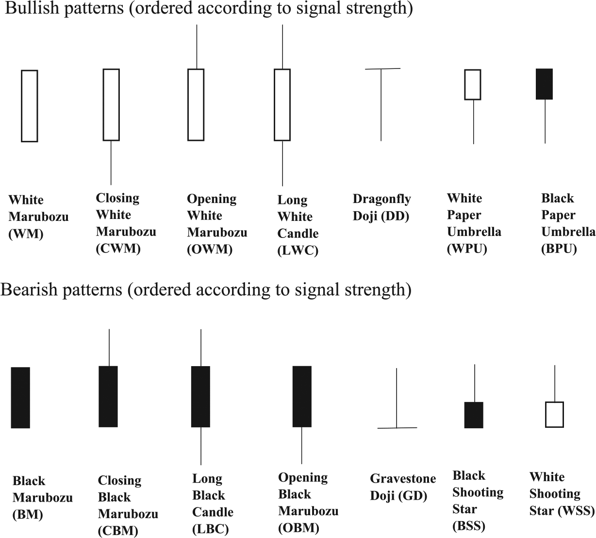
There are six bullish and six bearish 1-day patterns (Marshall et al., 2006). The bullish patterns are White Marubozu (WM), Closing White Marubozu (CWM), Opening White Marubozu (OWM), Long White Candle (LWC), Dragonfly Doji (DD), White Paper Umbrella (WPU), and Black Paper Umbrella (BPU). The bearish patterns are Black Marubozu (BM), Closing Black Marubozu (CBM), Long Black Candle (LBC), Opening Black Marubozu (OBM), Gravestone Doji (GD), Black Shooting Star (BSS), and White Shooting Star (WSS). The patterns are ordered according to signal strength.

There are five well-known 2-day bullish reversal patterns. They signal a change at the end of a downtrend. They are HP, bullish engulfing, piercing line (PL), BullH, and bullish kicking. There are also five well-known 2-day bearish reversal patterns. They signal a change at the end of an uptrend. They are descending hawk (DH), BearE, dark cloud cover (DCC), bearish harami, and bearish kicking.

There are four popular 3-day bullish reversal patterns. They signal a change at the end of a downtrend. They are three white soldier (TWS), three inside up (TIU), three outside up (TOU), and morning star (MS). There are four popular 3-day bearish reversal patterns. They signal a change at the end of an uptrend. They are three black crows (TBC), three inside down (TID), three outside down (TOD), and evening star (ES). All 3-day patterns are just extension of 2-day patterns with an extra 1 day for confirmation (Marshall et al., 2006).

In general, there are three approaches for an exit strategy. The first one is the MYR exit strategy introduced by Marshall et al. (2006). The second one is the CL exit strategy suggested by Caginalp and Laurent (1998). The third one is the Lu-Shiu-Liu (LSL) exit strategy proposed by Lu et al. (2012).

The MYR exit strategy assumes that investors liquidate their positions at the end of the holding period. In contrast, the CL exit strategy assumes that investors liquidate their positions during the holding period. As such, exit prices are average prices over the holding period. The typical holding periods are 1-day, 3-day, 5-day, and 10-day. The candlestick trading strategy should not be used for a period more than 10 days (Morris, 2006). Unlike other methods, the LSL exit strategy has a variable holding period. The LSL exit strategy assumes that investors buy (sell) on bullish (bearish) signal and liquidate their position when bearish (bullish) patterns happen. The purpose is to study profitability from a long-term perspective.

This article analyzes both MYR and CL exit strategies to evaluate the impacts of exit strategies on profitability of candlestick patterns. In fact, Lu et al. (2015) apply candlestick trading strategies to the 30 component stocks of the DJIA index over the 1992-2012 period and find that candlestick patterns with the CL exit strategy, but not with the MYR exit strategy, are profitable. They argue that the profitability of the CL exit strategy comes from a risk sharing mechanism when positions are unwound over the holding periods.

Though candlestick patterns with LSL exit strategy are interesting and Lu et al. (2012) even find that certain bullish reversal patterns generate positive abnormal returns in the Taiwan stock market, this article does not cover LSL exit strategy as we follow Morris’s recommendation that candlestick patterns is for a short-term period, not more than 10 days (Morris, 2006).

Candlestick Filtering

Morris (2006) defines candlestick filtering as a method of trading with candlestick patterns that is also supported by other technical indicators. He argues that filtering would improve trading profitability of candlesticks because it removes premature patterns and confirms trading signals. In fact, he finds that by filtering, the number of trades is significantly reduced but the average gain per trade increases.

A presignal is generated when a technical indicator gives an overbought or oversold signal. If the indicator gives an overbought (oversold) signal, then only bearish (bullish) candlestick patterns are filtered. This article uses Stochastics (%D), RSI, and MFI as candlestick filters. They have the advantage of ranging from 0 to 100 and give a clear overbought or oversold signal.

Stochastics (%D)

The stochastic oscillator indicates a relative position of a current price when compared with its price range over a period. The range is used as indicators of support and resistance levels. The oscillator itself is expressed as a percentage of this range. The number 0% and 100% would indicate the bottom and the peak within the range, respectively. The idea is based on the observation that turning points tend to be at the extremes of the recent price range. Normally, the numbers greater than the 80 level or lower than the 20 level are in an overbought or oversold territory, respectively.

The Stochastics are calculated by the following formulas:

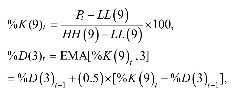
\begin{array}{l} % K (9)_{t} = \frac{P_{t} - L L (9)}{H H (9) - L L (9)} \times 100, \\ % D (3)_{t} = EMA [% K {(9)}_{t}, 3] \\ = % D {(3)}_{t - 1} + (0.5) \times [% K {(9)}_{t} - % D {(3)}_{t - 1}], \end{array}

where P_t = closing price at time “t,” LL(9) = lowest low price of previous 9 days, HH(9) = highest high price of previous 9 days, and EMA = exponential moving average.

The suggested lookback period for %K ranges from 5 to 21 days (Colby, 2003). The typical periods are 5, 9, and 14 days (Wikipedia, 2017b). The lookback period of 9 days is chosen in this case because of its closeness to the optimal parameter (for a long position) of 8 days as reported in Tharavanij, Siraprapasiri, and Rajchamaha (2015). The Stochastics %D is just an EMA of %K over a period of 3 days (Colby, 2003).

When Stochastics %D goes above 80, it gives an overbought signal and the sell filter is turned on. Any candlestick pattern that gives a sell signal when Stochastics %D is above 80 will be recognized as a filtered sell signal (Morris, 2006). Similarly, whenever Stochastics %D is below 20, it gives an oversold signal and the buy filter is turned on. Any candlestick pattern that gives a buy signal when Stochastics %D is below 20 will be recognized as a filtered buy signal (Morris, 2006).

RSI

The RSI indicates strength of upward price movements when compared with downward price movements. A high (low) stock price when compared with its recent past would have a high (low) RSI. The idea is that prices tend to be mean-reverting. If it rises or falls rapidly, it tends to reverse soon and returns to its mean. The RSI varies from 0 to 100. Normally, the numbers greater than the 70 level or lower than the 30 level are in an overbought or oversold territory, respectively (Colby, 2003).

The RSI is computed by the following steps. First, calculate the “U” and “D” variables according to the formulae stated below. Then, compute their exponential moving averages over 14 days to derive “Ua” and “Da” (Colby, 2003). The RSI is then calculated by the following equation:

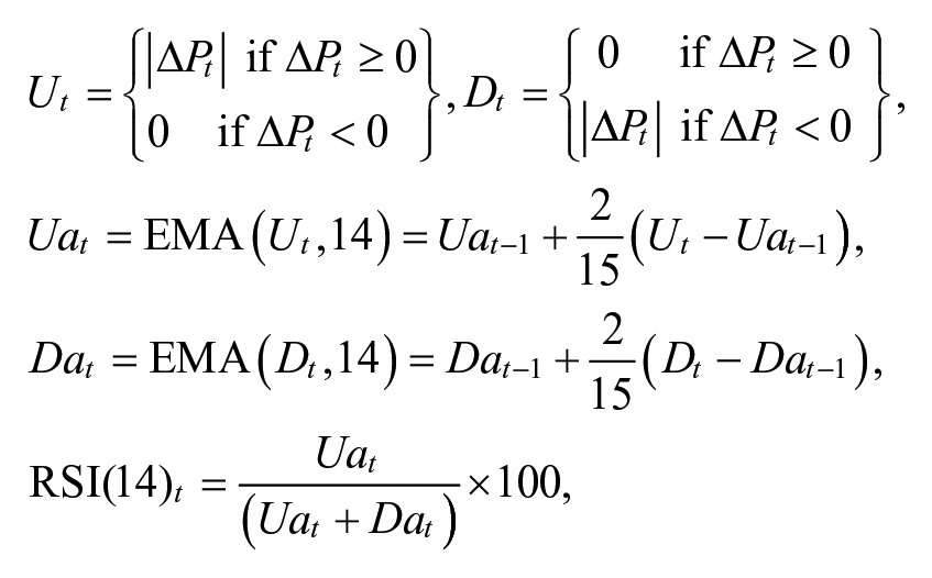
\begin{array}{l} U_{t} = {\begin{cases} | Δ P_{t} | if Δ P_{t} \geq 0 \\ 0 if Δ P_{t} < 0 \end{cases}}, D_{t} = {\begin{cases} 0 if Δ P_{t} \geq 0 \\ | Δ P_{t} | if Δ P_{t} < 0 \end{cases}}, \\ U a_{t} = EMA (U_{t}, 14) = U a_{t - 1} + \frac{2}{15} (U_{t} - U a_{t - 1}), \\ D a_{t} = EMA (D_{t}, 14) = D a_{t - 1} + \frac{2}{15} (D_{t} - D a_{t - 1}), \\ RSI (14)_{t} = \frac{U a_{t}}{(U a_{t} + D a_{t})} \times 100, \end{array}

where P_t = closing price at time “t.”

When RSI goes above 70, it gives an overbought signal and the sell filter is turned on. Any candlestick pattern that gives a sell signal when RSI is above 70 will be recognized as a filtered sell signal. Similarly, whenever RSI is below 30, it gives an oversold signal and the buy filter is turned on. Any candlestick pattern that gives a buy signal when RSI is below 30 will be recognized as a filtered buy signal.

MFI

The MFI is an approximation of a trading value over several days. It ranges from 0 to 100. Normally, the numbers greater than the 80 level or lower than the 20 level are in an overbought or oversold territory, respectively (Wikipedia, 2017a). The MFI is similar to the RSI in the sense that both measure positive changes against total changes. However, the MFI uses volume, whereas the RSI uses amounts of price changes.

The MFI is computed by the following steps. First, calculate the “typical price” according to the formula below. Then, multiply typical price and volume to derive the money flow. The money flow is grouped into positive and negative types. The positive (negative) money flow is defined as the 14-day summation of money flow when the typical price is increasing (decreasing). More specifically, the MFI is defined by the following equation:

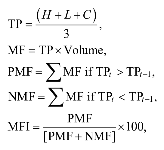
\begin{array}{l} TP = \frac{(H + L + C)}{3}, \\ MF = TP \times Volume, \\ PMF = \sum MF {if TP}_{t} > {TP}_{t - 1}, \\ NMF = \sum MF {if TP}_{t} < {TP}_{t - 1}, \\ MFI = \frac{PMF}{[PMF + NMF]} \times 100, \end{array}

where H, L, and C are high, low, and close price, respectively; TP = typical price; MF = money flow; PMF = positive money flow; and NMF = negative money flow.

When MFI goes above 80, it gives an overbought signal and the sell filter is turned on. Any candlestick pattern that gives a sell signal when MFI is above 80 will be recognized as a filtered sell signal. Similarly, whenever MFI is below 20, it gives an oversold signal and the buy filter is turned on. Any candlestick pattern that gives a buy signal when MFI is below 20 will be recognized as a filtered buy signal.

Method

The article applies a skewness adjusted t test (Johnson, 1978) to test the null hypothesis that the mean return is zero, and use the binomial test to test the null hypothesis that the winning rate is just 50%. The “Winning Rate” represents the proportion of positions with positive (negative) returns for bullish (bearish) signals.

As stock return distributions may not follow a normal distribution, the use of a skewness adjusted t test is more appropriate than a normal t test. The details of a return calculation, a skewness adjusted t test, and a binomial test are as follows.

Return Calculation

This article assumes that traders buy a stock at its opening price on the day after a bullish signal is detected. The stock is held over a fixed period and then sold at the closing price of a period. A holding period return is calculated. Similar to Marshall et al. (2006) and Zhu et al. (2016), this article uses raw returns instead of excess returns.

The returns calculated are holding period returns. The holding periods are 1, 3, 5, and 10 trading days. Then, this article calculates the means of all signaled returns of various stocks with the similar holding periods to determine the optimal holding periods for bullish and bearish signals. The return formulae depend on the employed exit strategy.

For the MYR exit strategy, the holding period continuous return is calculated by the following formula:

r_{t + h}^{c} = \ln C_{t + h} - \ln O_{t} .

For the CL exit strategy, the holding period continuous return is calculated by transforming a corresponding discrete return. The specific formula is the following:

\begin{array}{l} r_{t + h}^{d} = \frac{(\sum_{j = 1}^{h} \frac{C_{t + j}}{h} - O_{t})}{O_{t}}, \\ r_{t + h}^{c} = \ln (1 + r_{t + h}^{d}) . \end{array}

The superscript “c” denotes a continuous return, whereas “d” denotes a discrete one. The variable “h” is the number of trading days in a holding period. The variables “O” and “C” mean open and close prices, respectively.

Skewness Adjusted t Test

This article uses a skewness adjusted t test developed by Johnson (1978) to test profitability of candlestick patterns. The skewness adjusted t test is a valid nonparametric test even with biased distributions of return rates. This statistic is calculated using the following formula:

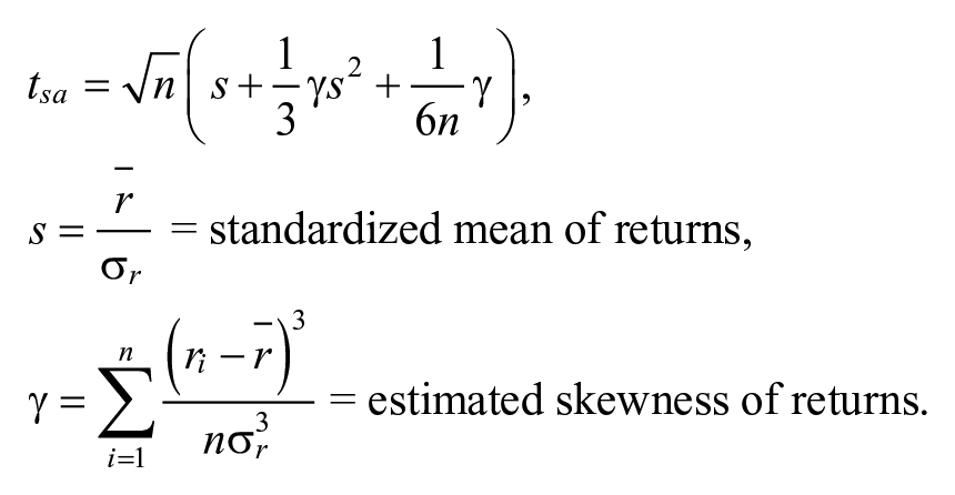
\begin{array}{l} t_{s a} = \sqrt{n} (s + \frac{1}{3} γ s^{2} + \frac{1}{6 n} γ), \\ s = \frac{\bar{r}}{σ_{r}} = standardized mean of returns, \\ γ = \sum_{i = 1}^{n} \frac{{(r_{i} - \bar{r})}^{3}}{n σ_{r}^{3}} = estimated skewness of returns . \end{array}

Bullish (bearish) signals are valid only if their mean returns are positively (negatively) significant. The one-tail t test is applied.

Neyman and Pearson (1928), and Pearson and Adyanthāya (1928, 1929) show that skewness has a greater impact on the distribution of the t statistics than kurtosis. A positive (negative) skewness in the return distribution would lead to a negatively (positively) skewed sampling distribution of t statistic. Sutton (1993) concludes that when the population distribution is asymmetrical, the use of Johnson’s statistics is preferred to the t test.

Binomial Test

The probability of correct predictions or winning probability is defined as the number of correct signals divided by the total observed signals. A binomial test is used to check whether candlestick patterns have a predictive power. The probability of correction should be higher than .5 if candlestick patterns signal the future short-term returns.

The exact interpretation of winning probabilities depends on the type of an exit strategy employed and whether it is a bullish or bearish pattern. In the case of MYR exit strategy, it is the probability that the holding period return would be positive (negative) for a bullish (bearish) signal. In the case of CL exit strategy, it is the probability that the average price over the holding period would be higher (lower) than the entry price, resulting in a positive (negative) holding period return for a bullish (bearish) signal.

The difference between the two means “np₀” (the expected number of success where p₀= .5) and “np” (the actual number) is divided by the standard deviation to get the Z statistic to test the null hypothesis:

Z = \frac{n (p - p_{0})}{σ} .

Using the central limit theorem, the Z statistic has a normal distribution. The standard error is given as follow:

σ = \sqrt{n p_{0} (1 - p_{0})} .

Data

Marshall et al. (2006) argue against the use of technical analysis on small or illiquid stocks because prospective profits are not economically significant. Therefore, this research studies stocks in the SET50 index. The sample period studied covers 10 years from July 3, 2006, to June 30, 2016. The SET50 constituents are stock used for calculating the index during July 1, 2016, to December 31, 2016. The more recent list is chosen for a relevancy reason. If component stocks do not have full records during the sample period, then only available records during the sample period are used. The data are from the SETSMART database. The list of stocks is reported in the appendix.

Empirical Results

This part discusses empirical results and test statistics, namely, adjusted t test and binomial test. Tables 1 to 6 provide statistics of each pattern. The overall picture is that both bullish and bearish candlestick reversal patterns are not useful. The mean returns of most patterns are not statistically different from zero. Even the ones with significant returns have relatively low mean returns (from 0.07% [BPU 3D-MYR] to 0.84% [BullH 5D-MYR]) compared with risks as measured by standard deviations (4.36% [BPU 3D-MYR], 7.04% [BullH 5D-MYR]). The binomial test results confirm the finding that normally candlestick patterns cannot reliably predict market directions. The rest of this part would be separated into results from single-day patterns, 2-day patterns, and 3-day patterns, consecutively.

Table 1.

Bullish Single Day Pattern.

Pattern	MYR				CL
Pattern	1D	3D	5D	10D	1D	3D	5D	10D
WM
n	5,592	5,590	5,585	5,577	5,592	5,590	5,585	5,577
M%	−0.08	0.02	0.09	0.31	−0.08	−0.01	0.04	0.17
SD%	2.89	4.33	5.30	7.29	2.89	3.37	3.80	4.71
t-adjusted	−2.10	0.43	1.21	3.22***	−2.10	−0.30	0.80	2.64***
Prob.	.39	.44	.45	.48	.39	.46	.48	.50
Z	−15.89	−9.44	−7.80	−3.28	−15.89	−5.35	−3.01	−0.50
CWM
n	10,848	10,833	10,805	10,778	10,848	10,833	10,805	10,778
M%	−0.17	−0.19	−0.27	−0.13	−0.17	−0.17	−0.18	−0.14
SD%	2.94	4.27	6.59	8.19	2.94	3.37	3.82	4.87
t-adjusted	−5.86	−4.59	−5.06	−1.67	−5.86	−5.25	−4.92	−3.11
Prob.	.40	.42	.44	.47	.40	.44	.45	.47
Z	−21.14	−15.80	−12.79	−7.15	−21.14	−12.19	−9.71	−5.55
OWM
n	10,471	10,455	10,450	10,437	10,471	10,455	10,450	10,437
M%	0.13	0.26	0.33	0.71	0.13	0.20	0.27	0.45
SD%	3.18	4.65	5.67	8.04	3.18	3.65	4.10	4.99
t-adjusted	4.28***	5.66***	5.89***	7.80***	4.28***	5.73***	6.78***	9.18***
Prob.	.45	.47	.49	.52	.45	.50	.51	.53
Z	−11.19	−6.41	−2.52	3.91***	−11.19	−0.13	2.05**	6.12***
LWC
n	14,830	14,791	14,770	14,750	14,830	14,791	14,770	14,750
M%	0.00	−0.01	0.07	0.30	0.00	0.01	0.05	0.18
SD%	3.26	5.79	6.65	8.70	3.27	3.83	4.39	5.46
t-adjusted	−0.08	−0.19	1.28*	3.78***	−0.08	0.41	1.44*	3.74***
Prob.	.43	.46	.47	.50	.43	.47	.49	.50
Z	−17.24	−9.55	−6.63	−0.89	−17.24	−6.85	−2.98	0.53
DD
n	2,905	2,905	2,902	2,896	2,905	2,905	2,902	2,896
M%	−0.15	−0.18	−0.24	−0.11	−0.15	−0.15	−0.17	−0.14
SD%	2.69	4.01	5.22	7.21	2.69	3.11	3.59	4.59
t-adjusted	−3.11	−2.44	−2.44	−0.86	−3.11	−2.70	−2.50	−1.64
Prob.	.37	.41	.42	.46	.37	.45	.46	.48
Z	−13.64	−10.11	−8.54	−4.01	−13.64	−5.88	−4.72	−2.68
WPU
n	921	920	918	915	921	920	918	915
M%	0.10	0.00	−0.25	−0.06	0.10	0.03	−0.06	−0.10
SD%	3.15	4.62	6.15	7.66	3.15	3.64	4.20	5.17
t-adjusted	0.99	−0.01	−1.26	−0.24	0.99	0.23	−0.42	−0.59
Prob.	.45	.45	.46	.50	.45	.47	.49	.49
Z	−3.06	−3.03	−2.24	−0.30	−3.06	−1.65	−0.40	−0.36
BPU
n	12,591	12,587	12,579	12,552	12,591	12,587	12,579	12,552
M%	−0.08	0.07	0.15	0.28	−0.08	0.00	0.06	0.18
SD%	3.12	4.36	5.50	7.43	3.12	3.46	3.91	4.84
t-adjusted	−2.93	1.89**	3.03***	4.20***	−2.93	−0.01	1.72**	4.27***
Prob.	.42	.46	.49	.50	.42	.48	.50	.51
Z	−16.89	−9.08	−3.18	−1.04	−16.89	−4.04	−0.24	3.28***

Note. The “n” is the number of signals in the sample for a particular holding period. The numbers of signals are not the same even for the same pattern because holding periods of some last signals are beyond our sample period and as such we do not include them in the calculation. The “M%” is the average holding period return. The “SD%” is the standard deviation of holding period returns. For bullish signals, the “t-adjusted” is the one-tail t test for the null hypothesis that μ ≤ 0. For bearish signals, the “t-adjusted” is the one-tail t test for the null hypothesis that μ ≥ 0. The “Prob.” is the winning probability that investors would earn positive profits by buying for bullish signals or selling for bearish signals. The “Z” is the one-tail Z test for the null hypothesis that winning probability ≤ .5. WM = White Marubozu; CWM = closing White Marubozu; OWM = opening White Marubozu; LWC = long white candle; DD = dragonfly doji; WPU = white paper umbrella; BPU = black paper umbrella; MYR = Marshall–Young–Rose; CL = Caginalp–Laurent.

*, **, *** denote statistical significance at 10%, 5% and 1%, respectively.

Table 2.

Bearish Single Day Pattern.

Pattern	MYR				CL
Pattern	1D	3D	5D	10D	1D	3D	5D	10D
BM
n	7,370	7,368	7,368	7,356	7,370	7,368	7,368	7,356
M%	0.02	0.12	0.24	0.43	0.02	0.08	0.14	0.28
SD%	2.94	4.51	5.67	7.61	2.94	3.45	3.96	4.98
t-adjusted	0.50	2.24	3.67	4.81	0.50	1.91	3.02	4.85
Prob.	.42	.43	.44	.44	.42	.47	.47	.47
Z	−13.14	−12.12	−11.11	−9.93	−13.14	−5.62	−4.73	−5.18
CBM
n	11,483	11,479	11,478	11,444	11,483	11,479	11,478	11,444
M%	0.09	0.24	0.42	0.67	0.09	0.20	0.28	0.44
SD%	3.17	4.65	5.69	7.69	3.17	3.63	4.10	5.11
t-adjusted	3.18	5.60	7.92	9.38	3.18	5.78	7.31	9.28
Prob.	.42	.43	.43	.44	.42	.46	.46	.45
Z	−16.38	−14.68	−14.88	−13.16	−16.38	−8.97	−9.07	−9.98
LBC
n	16,502	16,492	16,475	16,420	16,502	16,492	16,475	16,420
M%	0.00	0.13	0.30	0.47	0.00	0.08	0.16	0.33
SD%	4.03	5.29	6.22	8.95	4.03	4.41	4.78	5.62
t-adjusted	0.00	2.98	5.51	5.75	0.00	2.15	3.67	6.29
Prob.	.46	.46	.45	.45	.46	.48	.48	.47
Z	−10.24	−11.10	−12.55	−13.39	−10.24	−4.98	−4.46	−7.44
OBM
n	12,591	12,587	12,579	12,552	12,591	12,587	12,579	12,552
M%	−0.08	0.07	0.15	0.28	−0.08	0.00	0.06	0.18
SD%	3.12	4.36	5.50	7.43	3.12	3.46	3.91	4.84
t-adjusted	−2.93***	1.89	3.03	4.20	−2.93***	−0.01	1.72	4.27
Prob.	.46	.46	.45	.45	.46	.49	.49	.48
Z	−8.08	−9.30	−10.89	−10.10	−8.08	−1.58	−2.47	−4.27
GD
n	2,758	2,757	2,757	2,752	2,758	2,757	2,757	2,752
M%	0.11	0.22	0.36	0.75	0.11	0.18	0.25	0.46
SD%	2.63	4.24	5.31	7.15	2.63	3.23	3.75	4.69
t-adjusted	2.15	2.64	3.56	5.51	2.15	2.85	3.48	5.14
Prob.	.41	.42	.43	.42	.41	.47	.47	.46
Z	−9.71	−7.90	−7.29	−7.97	−9.71	−3.45	−2.95	−4.35
BSS
n	11,483	11,479	11,478	11,444	11,483	11,479	11,478	11,444
M%	0.09	0.24	0.42	0.67	0.09	0.20	0.28	0.44
SD%	3.17	4.65	5.69	7.69	3.17	3.63	4.10	5.11
t-adjusted	3.18	5.60	7.92	9.38	3.18	5.78	7.31	9.28
Prob.	.42	.43	.43	.44	.42	.46	.46	.45
Z	−16.38	−14.68	−14.88	−13.16	−16.38	−8.97	−9.07	−9.98
WSS
n	2,812	2,808	2,807	2,806	2,812	2,808	2,807	2,806
M%	0.20	0.42	0.63	0.94	0.20	0.33	0.45	0.68
SD%	3.26	4.52	5.34	9.17	3.26	3.63	3.98	4.80
t-adjusted	3.32	5.05	6.37	3.33	3.32	4.89	6.08	7.56
Prob.	.43	.45	.43	.42	.43	.47	.46	.45
Z	−6.94	−5.81	−7.76	−8.04	−6.94	−3.59	−4.59	−5.59

Note. The “n” is the number of signals in the sample for a particular holding period. The numbers of signals are not the same even for the same pattern because holding periods of some last signals are beyond our sample period and as such we do not include them in the calculation. The “M%” is the average holding period return. The “SD%” is the standard deviation of holding period returns. For bullish signals, the “t-adjusted” is the one-tail t test for the null hypothesis that μ ≤ 0. For bearish signals, the “t-adjusted” is the one-tail t test for the null hypothesis that μ ≥ 0. The “Prob.” is the winning probability that investors would earn positive profits by buying for bullish signals or selling for bearish signals. The “Z” is the one-tail Z test for the null hypothesis that winning probability ≤ .5. BM = Black Marubozu; CBM = closing Black Marubozu; LBC = long black candle; OBM = opening Black Marubozu; GD = gravestone doji; BSS = black shooting star; WSS = white shooting star; MYR = Marshall–Young–Rose; CL = Caginalp–Laurent.

*, **, *** denote statistical significance at 10%, 5% and 1%, respectively.

Table 3.

Bullish 2-Day Pattern.

Pattern	MYR				CL
Pattern	1D	3D	5D	10D	1D	3D	5D	10D
HP
n	380	380	380	379	380	380	380	379
M%	−0.10	0.04	0.21	0.07	−0.10	0.03	0.16	0.19
SD%	3.73	6.12	7.03	8.96	3.73	4.62	5.17	6.14
t-adjusted	−0.52	0.11	0.56	0.14	−0.52	0.13	0.57	0.59
Prob.	.46	.53	.52	.54	.46	.53	.56	.55
Z	−1.54	1.03	0.82	1.49*	−1.54	1.33*	2.36***	1.80**
BullE
n	275	274	274	274	275	274	274	274
M%	−0.46	−0.65	−0.49	−0.11	−0.46	−0.53	−0.51	−0.40
SD%	3.16	4.81	5.41	8.22	3.16	3.64	4.01	4.92
t-adjusted	−2.45	−2.34	−1.53	−0.21	−2.45	−2.50	−2.15	−1.35
Prob.	.38	.44	.45	.47	.38	.47	.47	.47
Z	−3.92	−1.93	−1.69	−0.97	−3.92	−1.09	−0.85	−1.09
PL
n	206	206	206	206	206	206	206	206
M%	−0.36	−0.86	−0.52	−0.06	−0.36	−0.66	−0.67	−0.48
SD%	3.26	5.04	5.90	9.17	3.26	3.75	4.13	5.29
t-adjusted	−1.57	−2.46	−1.27	−0.09	−1.57	−2.56	−2.34	−1.30
Prob.	.40	.40	.42	.47	.40	.42	.44	.44
Z	−2.93	−2.93	−2.23	−0.84	−2.93	−2.37	−1.67	−1.81
BullH
n	975	972	971	969	975	972	971	969
M%	0.53	0.64	0.84	0.53	0.53	0.60	0.74	0.80
SD%	3.97	5.74	7.04	8.52	3.97	4.59	5.18	5.99
t-adjusted	4.44***	3.5***2	3.78***	1.93**	4.44***	4.28***	4.63***	4.28***
Prob.	.50	.51	.53	.51	.50	.54	.55	.54
Z	0.10	0.71	1.96**	0.42	0.10	2.57***	3.18***	2.35***
BullK
n	275	274	274	274	275	274	274	274
M%	−0.46	−0.65	−0.49	−0.11	−0.46	−0.53	−0.51	−0.40
SD%	3.16	4.81	5.41	8.22	3.16	3.64	4.01	4.92
t-adjusted	−2.45	−2.34	−1.53	−0.21	−2.45	−2.50	−2.15	−1.35
Prob.	.38	.44	.45	.47	.38	.47	.47	.47
Z	−3.92	−1.93	−1.69	−0.97	−3.92	−1.09	−0.85	−1.09

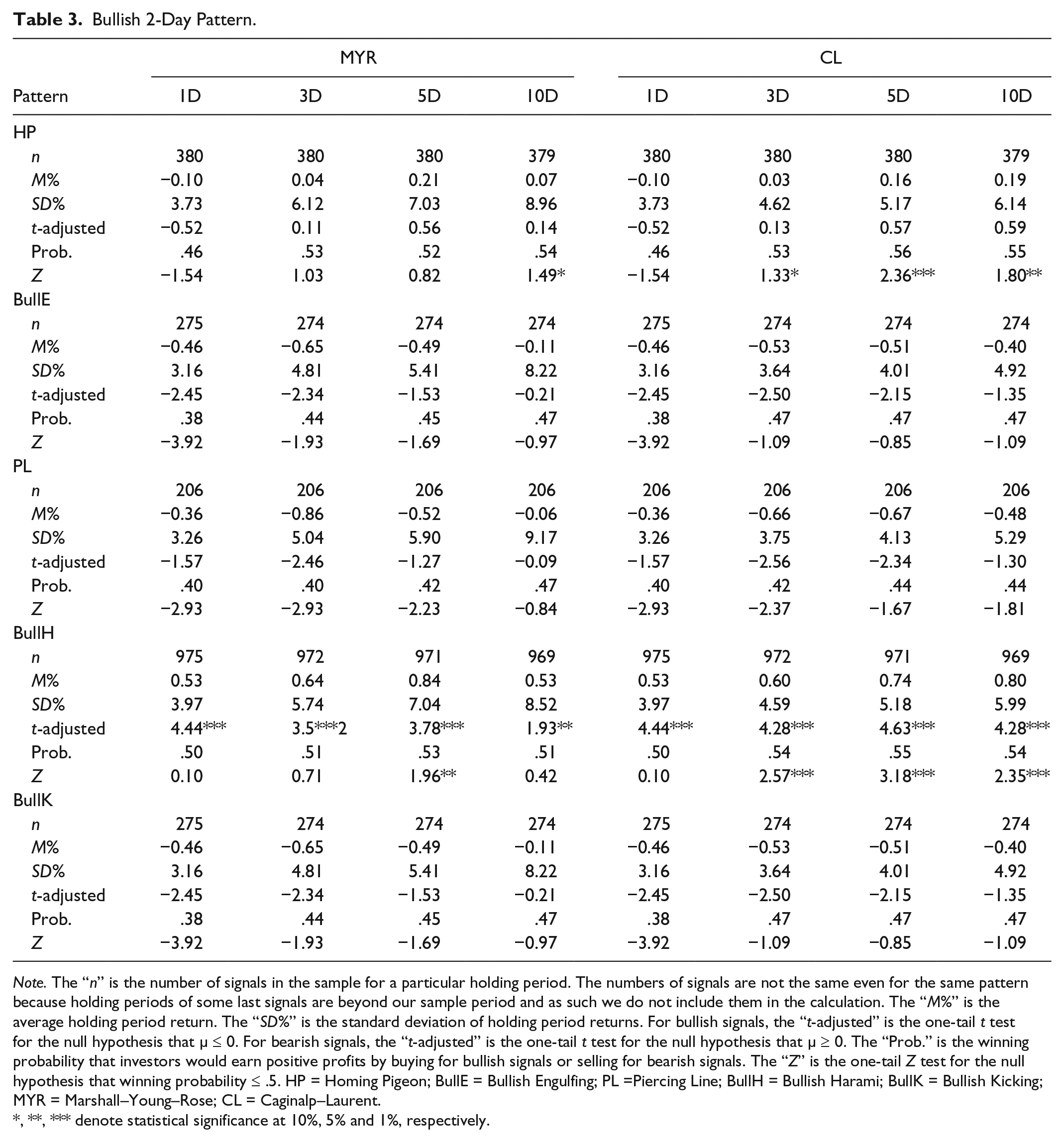
Note. The “n” is the number of signals in the sample for a particular holding period. The numbers of signals are not the same even for the same pattern because holding periods of some last signals are beyond our sample period and as such we do not include them in the calculation. The “M%” is the average holding period return. The “SD%” is the standard deviation of holding period returns. For bullish signals, the “t-adjusted” is the one-tail t test for the null hypothesis that μ ≤ 0. For bearish signals, the “t-adjusted” is the one-tail t test for the null hypothesis that μ ≥ 0. The “Prob.” is the winning probability that investors would earn positive profits by buying for bullish signals or selling for bearish signals. The “Z” is the one-tail Z test for the null hypothesis that winning probability ≤ .5. HP = Homing Pigeon; BullE = Bullish Engulfing; PL =Piercing Line; BullH = Bullish Harami; BullK = Bullish Kicking; MYR = Marshall–Young–Rose; CL = Caginalp–Laurent.

*, **, *** denote statistical significance at 10%, 5% and 1%, respectively.

Table 4.

Bearish 2-Day Pattern.

Pattern	MYR				CL
Pattern	1D	3D	5D	10D	1D	3D	5D	10D
DH
n	266	265	265	265	266	265	265	265
M%	−0.33	−0.39	−0.07	−0.02	−0.33	−0.34	−0.23	−0.08
SD%	3.65	4.36	5.33	8.62	3.65	3.82	3.87	4.94
t-adjusted	−1.65**	−1.51*	−0.21	−0.04	−1.65**	−1.57*	−1.01	−0.28
Prob.	.49	.55	.48	.48	.49	.52	.52	.49
Z	−0.25	1.54*	−0.80	−0.68	−0.25	0.80	0.68	−0.18
BearE
n	547	547	547	547	547	547	547	547
M%	0.26	0.26	0.69	1.06	0.26	0.25	0.41	0.74
SD%	3.33	4.60	5.85	7.76	3.33	3.59	4.07	5.01
t-adjusted	1.88	1.33	2.82	3.26	1.88	1.68	2.44	3.56
Prob.	.43	.44	.42	.44	.43	.45	.45	.45
Z	−3.12	−2.69	−3.72	−2.61	−3.12	−2.27	−2.18	−2.27
DCC
n	184	184	184	183	184	184	184	183
M%	−0.06	0.34	0.67	1.57	−0.06	0.14	0.36	0.89
SD%	3.03	4.59	5.61	7.53	3.03	3.54	4.04	4.92
t-adjusted	−0.26	1.00	1.63	2.92	−0.26	0.56	1.23	2.52
Prob.	.50	.49	.48	.42	.50	.51	.48	.46
Z	0.00	−0.15	−0.59	−2.29	0.00	0.15	−0.44	−1.11
BearH
n	997	996	996	994	997	996	996	994
M%	−0.02	−0.06	0.02	0.37	−0.02	0.01	0.03	0.14
SD%	3.24	4.67	5.78	7.55	3.24	3.69	4.16	5.06
t-adjusted	−0.16	−0.39	0.10	1.53	−0.16	0.09	0.20	0.88
Prob.	.50	.48	.50	.47	.50	.51	.50	.49
Z	−0.16	−1.20	−0.25	−1.59	−0.16	0.57	−0.25	−0.63
BearK
n	153	153	153	153	153	153	153	153
M%	0.04	0.16	0.17	0.24	0.04	0.10	0.15	0.29
SD%	3.04	4.07	4.22	6.57	3.04	3.26	3.34	3.90
t-adjusted	0.18	0.49	0.51	0.46	0.18	0.36	0.56	0.92
Prob.	.43	.44	.46	.49	.43	.47	.45	.49
Z	−1.70	−1.37	−1.05	−0.24	−1.70	−0.73	−1.21	−0.24

Note. The “n” is the number of signals in the sample for a particular holding period. The numbers of signals are not the same even for the same pattern because holding periods of some last signals are beyond our sample period and as such we do not include them in the calculation. The “M%” is the average holding period return. The “SD%” is the standard deviation of holding period returns. For bullish signals, the “t-adjusted” is the one-tail t test for the null hypothesis that μ ≤ 0. For bearish signals, the “t-adjusted” is the one-tail t test for the null hypothesis that μ ≥ 0. The “Prob.” is the winning probability that investors would earn positive profits by buying for bullish signals or selling for bearish signals. The “Z” is the one-tail Z test for the null hypothesis that winning probability ≤ .5. DH = descending hawk; BearE = bearish engulfing; DCC = dark cloud cover; BearH = bearish harami; BearK = bearish kicking; MYR = Marshall–Young–Rose; CL = Caginalp–Laurent.

*, **, *** denote statistical significance at 10%, 5% and 1%, respectively.

Table 5.

Bullish 3-Day Pattern.

Pattern	MYR				CL
Pattern	1D	3D	5D	10D	1D	3D	5D	10D
TWS
n	12	12	12	12	12	12	12	12
M%	−1.27	−0.55	−0.26	−0.33	−1.27	−0.99	−0.54	0.16
SD%	3.67	4.79	4.94	7.80	3.67	4.16	3.82	4.52
t-adjusted	−1.24	−0.37	−0.15	−0.21	−1.24	−0.81	−0.45	0.13
Prob.	.42	.42	.33	.58	.42	.42	.25	.33
Z	−0.58	−0.58	−1.15	0.58	−0.58	−0.58	−1.73	−1.15
TIU
n	179	178	177	177	179	178	177	177
M%	0.16	0.67	0.58	0.34	0.16	0.41	0.46	0.39
SD%	4.26	7.37	7.82	9.57	4.26	5.37	6.15	7.04
t-adjusted	0.53	1.28*	1.05	0.47	0.53	1.09	1.06	0.76
Prob.	.40	.50	.46	.50	.40	.45	.49	.53
Z	−2.62	0.00	−1.13	0.08	−2.62	−1.35	−0.38	0.83
TOU
n	97	96	96	96	97	96	96	96
M%	0.28	0.13	−0.12	−0.39	0.28	0.18	0.08	−0.14
SD%	2.54	3.59	4.96	7.33	2.54	2.87	3.17	4.18
t-adjusted	1.05	0.35	−0.26	−0.55	1.05	0.60	0.25	−0.35
Prob.	.47	.49	.49	.51	.47	.51	.52	.51
Z	−0.51	−0.20	−0.20	0.20	−0.51	0.20	0.41	0.20
MS
n	200	199	199	199	200	199	199	199
M%	−0.46	−0.69	−0.70	−1.11	−0.46	−0.54	−0.58	−0.57
SD%	2.93	4.72	5.39	10.02	2.93	3.58	3.95	5.19
t-adjusted	−2.20	−2.09	−1.86	−1.71	−2.20	−2.11	−2.07	−1.60
Prob.	.37	.42	.45	.50	.37	.39	.43	.48
Z	−3.68	−2.20	−1.35	0.07	−3.68	−3.19	−1.91	−0.50

Note. The “n” is the number of signals in the sample for a particular holding period. The numbers of signals are not the same even for the same pattern because holding periods of some last signals are beyond our sample period and as such we do not include them in the calculation. The “M%” is the average holding period return. The “SD%” is the standard deviation of holding period returns. For bullish signals, the “t-adjusted” is the one-tail t test for the null hypothesis that μ ≤ 0. For bearish signals, the “t-adjusted” is the one-tail t test for the null hypothesis that μ ≥ 0. The “Prob.” is the winning probability that investors would earn positive profits by buying for bullish signals or selling for bearish signals. The “Z” is the one-tail Z test for the null hypothesis that winning probability ≤ .5. TWS = three white soldiers; TIU = three inside up; TOU = three outside up; MS = morning star; MYR = Marshall–Young–Rose; CL = Caginalp–Laurent.

*, **, *** denote statistical significance at 10%, 5% and 1%, respectively.

Table 6.

Bearish 3-Day Pattern.

Pattern	MYR				CL
Pattern	1D	3D	5D	10D	1D	3D	5D	10D
TBC
n	30	30	30	30	30	30	30	30
M%	0.51	1.38	1.57	2.66	0.51	0.90	1.07	1.90
SD%	2.60	3.91	4.61	8.63	2.60	2.85	3.33	5.26
t-adjusted	1.12	2.03	2.01	1.88	1.12	1.79	1.90	2.34
Prob.	.33	.30	.30	.33	.33	.37	.33	.30
Z	−1.83	−2.19	−2.19	−1.83	−1.83	−1.46	−1.83	−2.19
TID
n	147	147	147	147	147	147	147	147
M%	0.23	0.33	0.61	2.16	0.23	0.27	0.36	1.00
SD%	3.05	3.86	5.07	7.72	3.05	3.27	3.65	4.71
t-adjusted	0.93	1.05	1.49	3.71	0.93	1.01	1.21	2.66
Prob.	.46	.45	.43	.40	.46	.49	.49	.40
Z	−0.91	−1.24	−1.73	−2.39	−0.91	−0.25	−0.25	−2.39
TOD
n	560	560	560	559	560	560	560	559
M%	−0.10	−0.09	0.05	0.45	−0.10	−0.10	−0.05	0.18
SD%	3.06	4.61	5.32	7.87	3.06	3.54	3.89	4.91
t-adjusted	−0.77	−0.45	0.24	1.37	−0.77	−0.66	−0.32	0.88
Prob.	.48	.49	.49	.46	.48	.53	.52	.50
Z	−1.18	−0.51	−0.34	−1.82	−1.18	1.61	0.93	−0.04
ES
n	209	209	209	209	209	209	209	209
M%	−0.23	−0.17	−0.22	0.14	−0.23	−0.27	−0.24	−0.06
SD%	2.83	4.13	4.85	7.01	2.83	3.18	3.48	4.28
t-adjusted	−1.16	−0.58	−0.68	0.28	−1.16	−1.23	−1.00	−0.21
Prob.	.47	.47	.47	.47	.47	.51	.48	.48
Z	−0.76	−0.76	−0.76	−0.90	−0.76	0.21	−0.62	−0.62

Note. The “n” is the number of signals in the sample for a particular holding period. The numbers of signals are not the same even for the same pattern because holding periods of some last signals are beyond our sample period and as such we do not include them in the calculation. The “M%” is the average holding period return. The “SD%” is the standard deviation of holding period returns. For bullish signals, the “t-adjusted” is the one-tail t test for the null hypothesis that μ ≤ 0. For bearish signals, the “t-adjusted” is the one-tail t test for the null hypothesis that μ ≥ 0. The “Prob.” is the winning probability that investors would earn positive profits by buying for bullish signals or selling for bearish signals. The “Z” is the one-tail Z test for the null hypothesis that winning probability ≤ .5. TBC = three black crows; TID = three inside down; TOD = three outside down; ES = evening star; MYR = Marshall–Young–Rose; CL = Caginalp–Laurent.

*, **, *** denote statistical significance at 10%, 5% and 1%, respectively.

In the case of bullish single-day patterns, most candlestick patterns could not generate statistically significant positive mean returns. The ones that did are WM, OWM, LWC, and BPU. Only OWM has significant mean returns over all horizons. The BPU comes close as its mean returns are significant over all horizons except for 1 day. The WM and LWC have significant mean returns only for a 10-day holding horizon. The binomial test results show that the winning probability is normally not significant. The notable exception is the OWM for a 5- or 10-day holding horizon. Overall, the OWM has the best performance. Its adjusted t statistics are highly significant in all holding periods and for both MYR and CL exit strategies. The mean returns are also the highest. This is a surprise given that according to candlestick textbooks (e.g., Morris, 2006; Nison, 1991) this pattern does not give the strongest bullish signal (in fact, that one belongs to WM). The OWM, in fact, only gives the third strongest bullish signal (after WM and CWM). This may indicate that signal strength does not necessarily follow what is specified in candlestick textbooks and may vary among stocks and stock markets. Interestingly, the supposedly second strongest bullish signal, the CWM pattern, in fact, has highly significant negative mean returns. The binomial test confirms the above result as the Z statistics are highly negatively significant. Traders could make a profit (at least before transaction costs) on average from selling when the CWM pattern happens instead of buying as suggested in candlestick textbooks.

In the case of bearish 1-day patterns, all patterns except OBM do not have significant negative mean returns. Even for the OBM pattern, the negative mean return (–0.08%) is significant only for the holding period of just 1 day. In addition, the binomial test results are all insignificant. This implies that none of the bearish single-day patterns could reliably predict market downturns. However, similar to the bullish CWM pattern case described above, most bearish 1-day patterns, like CBM, LBC, GD, BSS, and WSS, do not have negative mean returns as expected but surprisingly have highly significant positive mean returns. This implies that traders could make a profit (at least before transaction costs) on average from buying instead of selling as suggested in candlestick textbooks. Basically, they behave more like bullish signals than bearish ones. In addition, their binomial test results are negatively significant, meaning that these patterns do, indeed, predict market upturns.

In the case of bullish 2-day patterns, only BullH has significant positive mean returns over all horizons. Returns of all other bullish 2-day patterns are not significant. For bearish 2-day patterns, none have significant mean returns except DH with 1- to 3-day horizons. The winning probabilities are also not significant. Unlike in the case of 1-day patterns, almost all 2-day patterns have mean returns that are neither positively or negatively significant. The only exceptions are BearE and DCC which have positively significant mean returns over a period of 5 to 10 days.

In the case of bullish 3-day patterns, only TIU has a significant (at a 10% level) positive mean returns over three trading days with MYR exit strategy. All winning probabilities are not significant. For bearish 3-day patterns, none have significant negative mean returns. Interestingly, like the case of bearish single-day patterns, the TBC and TID patterns have significant positive mean returns (for a 10-day horizon) instead of expected negative ones. They behave, in fact, more like bullish signals.

In summary, most candlestick patterns are not very useful in terms of investment timing. Even the ones with statistically significant returns do have high risks in terms of standard deviations. For example, the OWM pattern, a single-day bullish pattern, has the highest holding period return of 0.71% (10 days with MYR) with the associated standard deviation of 8.04%. In addition, the signal strength or direction (bullish or bearish) do not necessarily follow those suggested in candlestick textbooks. For example, the CBM pattern, a 1-day bearish pattern, has no significant negative mean returns as expected but instead has significant positive mean returns. It behaves more like a bullish pattern. In terms of exit strategies (MYR vs. CL), this article does not find much difference but the general observation that mean returns and standard deviations of MYR tend to be higher than those of CL. This may reflect the fact that the CL exit strategy allows traders to divesting evenly over holding periods.

Filtered Candlestick Patterns

The results from filtered patterns are reported in Supplementary Tables S1 to S6, Tables S7 to S13, and Tables S14 to S18 in the supplementary appendix for filtering with Stochastics (%D), RSI, and MFI, respectively. The overall picture is that even with filtering, candlestick patterns are still not useful. Among profitable unfiltered patterns, filtering reduces the number of trades dramatically, but the average mean returns and winning probabilities do not significantly increase except for the LWC with RSI filter. Among unprofitable unfiltered patterns, they are still not profitable even with filters. The binomial test results reveal that even with filtering, most candlestick patterns cannot reliably predict market directions. The rest of this part would be separated into results from 1-, 2-, and 3-day patterns, consecutively.

Among single-day bullish patterns, the best strategy changes from the OWM (unfiltered) to the LWC (filtered). The second best strategy also changes from the BPU (unfiltered) to the WPU (with Stochastics %D filter). The RSI filter increases LWC profitability drastically from less than 1% to higher than 1% in most cases; however, standard deviations also increase. Similar to the unfiltered case, nearly all filtered single-day bearish patterns could not generate significant negative returns. The binomial tests confirm the result that they could not reliably predict market downturns.

Among 2-day bullish patterns, the best unfiltered and filtered strategy is consistently the BullH. The number of trades decreases a little by filtering while average returns and risks remain relatively the same. Among 2-day bearish patterns, the DH strategy is the only profitable strategy with significant negative mean returns. Similar to the 2-day bullish case, the number of trades decreases a little by filtering while average returns and risks remain relatively the same.

Among 3-day bullish or bearish patterns, none generate profits. Filtering does not improve profitability or prediction accuracy of a 3-day pattern.

Conclusion

This article investigates the profitability of candlestick bullish and bearish reversal patterns when applied to component stocks of the SET50 index for the 10-year period from July 3, 2006, to June 30, 2016. The holding periods are 1 day, 3 days, 5 days, and 10 days. Two exit strategies are studied. One is the MYR exit strategy (Marshall et al., 2006) and the other is the CL exit strategy (Caginalp & Laurent, 1998). The MYR applies a prespecified date to exit the market. In contrast, the CL sets an exit price equal to an average holding period closing price, assuming that investors liquidate their positions evenly within this period. In terms of methodology, this study uses the skewness adjusted t test (Johnson, 1978) and the binomial test.

The statistical analysis finds little use of both bullish and bearish candlestick reversal patterns since the mean returns of most patterns are not statistically different from zero. Even the ones with statistically significant returns do have high risks in terms of standard deviations. The binomial test results also indicate that candlestick patterns cannot reliably predict market directions.

Furthermore, this study finds that the signal strength or direction (bullish or bearish) do not necessary follow those suggested in candlestick textbooks. For example, the CBM pattern, a single-day bearish pattern, has no significant negative mean returns as expected but instead has positive mean returns. In terms of exit strategies (MYR vs. CL), this article observes that results from MYR tend to have both higher mean returns and higher standard deviations compared with those from CL. In addition, this article finds that filtering either by Stochastics (%D), RSI, or MFI generally does not increase profitability nor prediction accuracy of candlestick patterns.

This article has the following limitations. First, we do not investigate the roles of trend, support, and resistance lines. Second, our sample includes only components of the largest 50 stocks in the SET. It is possible that candlestick pattern is more effective for smaller capitalized stocks. These could be the topic for future studies.

Footnotes

Appendix

Table A1.

SET50 CONSTITUENTS (as announced on June 17, 2016).

For Calculating the Index During July 1, 2016, to December 31, 2016.

No.	Ticker	Company	Sector	First day in sample	Observation
1	ADVANC	ADVANCED INFO SERVICE	Information & Communication Technology	July 3, 2006	2,443
2	AOT	AIRPORTS OF THAILAND	Transportation & Logistics	July 3, 2006	2,443
3	BA	BANGKOK AIRWAYS	Transportation & Logistics	November 3, 2014	403
4	BANPU	BANPU	Energy & Utilities	July 3, 2006	2,443
5	BBL	BANGKOK BANK	Banking	July 3, 2006	2,443
6	BCP	BANGCHAK PETROLEUM	Energy & Utilities	July 3, 2006	2,443
7	BDMS	BANGKOK DUSIT MEDICAL SERVICES	Health Care Services	July 3, 2006	2,443
8	BEC	BEC WORLD	Media & Publishing	July 3, 2006	2,443
9	BEM	BANGKOK EXPRESSWAY AND METRO	Transportation & Logistics	July 3, 2006	2,434
10	BH	BUMRUNGRAD HOSPITAL	Health Care Services	July 3, 2006	2,443
11	BLA	BANGKOK LIFE ASSURANCE	Insurance	October 28, 2009	1,628
12	BTS	BTS GROUP HOLDING	Transportation & Logistics	July 3, 2006	2,319
13	CBG	CARABAO GROUP	Food and Beverage	July 3, 2006	389
14	CENTEL	CENTRAL PLAZA HOTEL	Tourism & Leisure	July 3, 2006	2,440
15	CK	CH KARNCHANG	Construction Services	July 3, 2006	2,443
16	CPALL	CP ALL	Commerce	July 3, 2006	2,442
17	CPF	CHAROEN POKPHAND FOODS	Food and Beverage	July 3, 2006	2,442
18	CPN	CENTRAL PATTANA	Property Development	July 3, 2006	2,443
19	DELTA	DELTA ELECTRONICS (THAILAND)	Electronic Components	July 3, 2006	2,443
20	DTAC	TOTAL ACCESS COMMUNICATION	Information & Communication Technology	June 22, 2007	2,204
21	EGCO	ELECTRICITY GENERATING	Energy & Utilities	July 3, 2006	2,443
22	GLOW	GLOW ENERGY	Energy & Utilities	July 3, 2006	2,443
23	GPSC	GLOBAL POWER SYENERGY	Energy & Utilities	May 18, 2015	276
24	HMPRO	HOME PRODUCE CENTER	Commerce	July 3, 2006	2,443
25	INTUCH	INTOUCH HOLDING	Information & Communication Technology	July 3, 2006	2,442
26	IRPC	IRPC	Energy & Utilities	July 3, 2006	2,443
27	IVL	INDORAMA VENTURES	Petrochemicals & Chemicals	February 5, 2010	1,560
28	KBANK	KASIKORNBANK	Banking	July 3, 2006	2,443
29	KCE	KCE ELECTRONICS	Electronic Components	July 3, 2006	2,443
30	KTB	KRUNG THAI BANK	Banking	July 3, 2006	2,443
31	LH	LAND AND HOUSES	Property Development	July 3, 2006	2,443
31	MINT	MINOR INTERNATIONAL	Food and Beverage	July 3, 2006	2,442
33	MTLS	MUANGTHAI LEASING	Finance and Securities	November 26, 2014	386
34	PS	PRUKSA REAL ESTATE	Property Development	July 3, 2006	2,443
35	PTT	PTT	Energy & Utilities	July 3, 2006	2,441
36	PTTEP	PTT EXPLORATION AND PRODUCTION	Energy & Utilities	July 3, 2006	2,443
37	PTTGC	PTT GLOBAL CHEMICAL	Petrochemicals & Chemicals	February 1, 2008	2,044
38	ROBINS	ROBINSON DEPARTMENT STORE	Commerce	July 3, 2006	2,431
39	SAWAD	SRISAWAD POWER	Finance and Securities	May 8, 2014	524
40	SCB	SIAM COMMERCIAL BANK	Banking	July 3, 2006	2,443
41	SCC	SIAM CEMENT	Construction Materials	July 3, 2006	2,443
42	TASCO	TIPCO ASPHALT	Construction Materials	July 3, 2006	2,441
43	TCAP	THANACHART CAPITAL	Banking	July 3, 2006	2,442
44	TMB	TMB BANK	Banking	July 3, 2006	2,442
45	TOP	THAI OIL	Energy & Utilities	July 3, 2006	2,443
46	TPIPL	TPI POLENE	Construction Materials	July 3, 2006	2,438
47	TRUE	TRUE CORPORATION	Information & Communication Technology	July 3, 2006	2,443
48	TTW	TTW	Energy & Utilities	May 22, 2008	1,980
49	TU	THAI UNION GROUP	Food and Beverage	July 3, 2006	2,443
50	WHA	WHA CORPORATION	Property Development	November 8, 2012	887

Note. SET50 = the 50 largest capitalization stocks in the stock exchange of Thailand.

Acknowledgements

We would like to thank Mahidol University and the College of Management for providing databases for this research.

Declaration of Conflicting Interests

The author(s) declared no potential conflicts of interest with respect to the research, authorship, and/or publication of this article.

Funding

The author(s) received no financial support for the research, authorship, and/or publication of this article.

Author Biographies

Piyapas Tharavanij is an assistant professor of finance at CMMU. His research interests are in the fields of investment and corporate finance.

Vasan Siraprapasiri is a finance faculty at CMMU. His research interests are in the fields of security valuation and corporate strategy.

Kittichai Rajchamaha is an entrepreneurship faculty at CMMU. His research interests are in the fields of entrepreneurial finance and managerial accounting.

References

Brown

D. P.

Jennings

R. H.

(1989). On technical analysis. Review of Financial Studies, 2, 527-551.

Caginalp

Laurent

(1998). The predictive power of price patterns. Applied Mathematical Finance, 5, 181-205.

Chen

Bao

Zhou

(2016). The predictive power of Japanese candlestick charting in Chinese stock market. Physica A: Statistical Mechanics and Its Applications, 457, 148-165.

Colby

R. W.

(2003). The encyclopedia of technical market indicators (2nd ed.). New York: McGraw-Hill.

DeLong

J. B.

Shleifer

Summers

L. H.

(1990). Positive feedback investment strategies and destabilizing rational speculation. Journal of Finance, 45, 379-395.

Duvinage

Mazza

Petitjean

(2013). The intra-day performance of market timing strategies and trading systems based on Japanese candlesticks. Quantitative Finance, 13, 1059-1070.

Fama

E. F.

(1970). Efficient capital markets: A review of theory and empirical work. Journal of Finance, 25, 383-417.

Froot

K. A.

Scharftstein

D. S.

Stein

J. C.

(1992). Herd on the street: Informational inefficiencies in a market with short-term speculation. Journal of Finance, 47, 1461-1484.

Goo

Y.-J.

Chen

D.-H.

Chang

Y.-W.

(2007). The application of Japanese candlestick trading strategies in Taiwan. Investment Management and Financial Innovations, 4(4), 49-79.

10.

Grossman

S. J.

Stiglitz

J. E.

(1980). On the impossibility of informationally efficient markets. American Economic Review, 70, 393-408.

11.

Horton

M. J.

(2009). Stars, crows, and doji: The use of candlesticks in stock selection. Quarterly Review of Economics and Finance, 49, 283-294.

12.

Johnson

N. J.

(1978). Modified t tests and confidence intervals for asymmetrical populations. Journal of the American Statistical Association, 73, 536-544.

13.

Levy

R. A.

(1971). The predictive significance of five-point chart patterns. Journal of Business, 44, 316-323.

14.

T.-H.

(2014). The profitability of candlestick charting in the Taiwan stock market. Pacific-Basin Finance Journal, 26, 65-78.

15.

T.-H.

Chen

Y.-C.

Hsu

Y.-C.

(2015). Trend definition or holding strategy: What determines the profitability of candlestick charting? Journal of Banking & Finance, 61, 172-183.

16.

T.-H.

Shiu

Y.-M.

(2012). Tests for two-day candlestick patterns in the emerging equity market of Taiwan. Emerging Markets Finance & Trade, 48(Suppl. 1), 41-57.

17.

T.-H.

Shiu

Y.-M.

Liu

T.-C.

(2012). Profitable candlestick trading strategies—The evidence from a new perspective. Review of Financial Economics, 21, 63-68.

18.

Marshall

B. R.

Cahan

R. H.

Cahan

J. M.

(2008). Does intraday technical analysis in the U.S. equity market have value? Journal of Empirical Finance, 15, 199-210.

19.

Marshall

B. R.

Young

M. R.

Cahan

(2008). Are candlestick technical trading strategies profitable in the Japanese equity market? Review of Quantitative Finance and Accounting, 31, 191-207.

20.

Marshall

B. R.

Young

M. R.

Rose

L. C.

(2006). Candlestick technical trading strategies: Can they create value for investors? Journal of Banking & Finance, 30, 2303-2323.

21.

Marshall

B. R.

Young

M. R.

Rose

L. C.

(2007). Market timing with candlestick technical analysis. Journal of Financial Transformation, 20, 18-25.

22.

Menkhoff

(2010). The use of technical analysis by fund managers: International evidence. Journal of Banking & Finance, 34, 2573-2586.

23.

Morris

G. L.

(2006). Candlestick charting explained: Timeless techniques for trading stocks and futures (3rd ed.). New York, NY: McGraw-Hill.

24.

Neyman

Pearson

E. S.

(1928). On the use and interpretation of certain test criteria for purposes of statistical inference: Part I. Biometrika, 20A, 175-240.

25.

Nison

(1991). Japanese candlestick charting techniques. New York, NY: Institute of Finance.

26.

Pearson

E. S.

Adyanthāya

N. K.

(1928). The distribution of frequency constants in small samples from symmetrical populations. Biometrika, 20, 356-360.

27.

Pearson

E. S.

Adyanthāya

N. K.

(1929). The distribution of frequency constants in small samples from non-normal symmetrical and skew populations. Biometrika, 21, 259-286.

28.

Shiu

Y.-M.

T.-H.

(2011). Pinpoint and synergistic trading strategies of candlesticks. International Journal of Economics and Finance, 3, 234-244.

29.

Sutton

C. D.

(1993). Computer-intensive methods for tests about the mean of an asymmetrical distribution. Journal of the American Statistical Association, 88, 802-808.

30.

Tharavanij

Siraprapasiri

Rajchamaha

(2015). Performance of technical trading rules: Evidence from Southeast Asian stock markets. SpringerPlus, 4(552), 1-40.

31.

Wikipedia. (2017a). Money flow index. Retrieved from https://en.wikipedia.org/wiki/Money_flow_index

32.

Wikipedia. (2017b). Stochastic oscillator. Retrieved from https://en.wikipedia.org/wiki/Stochastic_oscillator

33.

Zhu

Atri

Yegen

(2016). Are candlestick trading strategies effective in certain stocks with distinct features? Pacific-Basin Finance Journal, 37, 116-127.

Supplementary Material

Please find the following supplemental material available below.

For Open Access articles published under a Creative Commons License, all supplemental material carries the same license as the article it is associated with.

For non-Open Access articles published, all supplemental material carries a non-exclusive license, and permission requests for re-use of supplemental material or any part of supplemental material shall be sent directly to the copyright owner as specified in the copyright notice associated with the article.

0.00 MB

0.96 MB

0.17 MB

Profitability of Candlestick Charting Patterns in the Stock Exchange of Thailand

Abstract

Keywords

Introduction

Literature Review

Theory

Empirical Studies

Candlestick Methodology

Candlestick Charting

Trend Definitions

Candlestick Patterns

Candlestick Filtering

Stochastics (%D)

RSI

MFI

Method

Return Calculation

Skewness Adjusted t Test

Binomial Test

Data

Empirical Results

Filtered Candlestick Patterns

Conclusion

Footnotes

Appendix

Acknowledgements

Declaration of Conflicting Interests

Funding

Author Biographies

References

Supplementary Material