Sage Journals: Discover world-class research

Abstract

Latent basis growth modeling is a flexible version of the growth curve modeling, in which it allows the basis coefficients of the model to be freely estimated, and thus the optimal growth trajectories can be determined from the observed data. In this article, Bayesian estimation methods are applied for latent basis growth modeling. Because the latent basis coefficients are important parameters that determine the growth pattern in latent basis growth models, we evaluate the impact of different priors for the basis coefficients on parameter recovery and model estimation. Noninformative priors, informative priors with varying levels of accuracy and precision, and data-dependent priors are considered. In addition, the issue of model specification is treated as a prior selection procedure. The impact of model misspecification and priors for model parameters are investigated simultaneously. A Monte Carlo simulation study is conducted and suggests that misspecified models adversely affect the parameter estimation much more than inaccurate priors. Recommendations on prior selection in latent basis growth models are given based on the simulation results. A real data example on the development of schoolchildren’s reading ability is also provided to illustrate the comparison among different sets of priors.

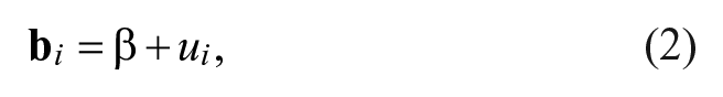
Keywords

Bayesian estimation Bayesian priors latent basis growth models growth curve models model misspecification

Longitudinal data are commonly used in social and behavioral sciences to study change over time. Latent growth curve models are powerful tools to analyze longitudinal data and can directly investigate intraindividual change over time and interindividual difference in intraindividual change (McArdle & Nesselroade, 2014). Latent basis growth models (LBGMs) are a type of latent growth curve models. This type of growth curve models typically fixes the basis coefficients/loadings for the first and last waves of data for identification purposes, while allowing other basis coefficients/loadings to be freely estimated. In this way, the optimal growth trajectory, either linear or nonlinear, can be determined by observed data (e.g., McArdle & Nesselroade, 2014; Meredith & Tisak, 1990). Because of such a flexibility, there is an increasing number of research implementing LBGMs to analyze longitudinal data (e.g., Phan, 2013).

In estimating LBGMs, Bayesian approach has many advantages. First, in longitudinal data, developmental complexities such as unequally spaced occasions, nonlinear or compound trajectories, or nonnormally distributed repeated measures arise commonly (e.g., Curran, Obeidat, & Losardo, 2010; Grimm & Ram, 2009). Even after a complicated transformation of the data, Bayesian inferences can still be easily drawn based on posterior distributions of model parameters (Gelman, Carlin, Stern, & Rubin, 2015). Second, Bayesian methods can be applied to estimate complex models. With a complicated data structure, Bayesian posteriors of model parameters can be approximated using a simulation-based Markov Chain Monte Carlo (MCMC) algorithm (e.g., Dunson, 2000; Lu & Zhang, 2014). Third, previous literature suggested that Bayesian methods are more plausible than the maximum likelihood (ML) estimation when sample size is small, because Bayesian inference is not based on asymptotic theory, and limiting approximations are not needed for Bayesian inferences of posterior distributions (e.g., Casella & Berger, 2001; Hoogland & Boomsma, 1998; Schafer, 1997; Scheines, Hoijtink, & Boomsma, 1999). More specifically, Scheines et al. (1999) showed that Bayesian estimation outperforms ML estimation when sample size is small. Lee and Chang (2000) demonstrated that the MCMC algorithm provides a smaller prediction error such as the mean squared deviation and is slightly more efficient with small sample growth data.

Furthermore, the improvement in computing powers and accessibility to Bayesian software have popularized the Bayesian approach in estimating growth curve models. Consequently, more and more researchers conduct growth curve analysis from a Bayesian perspective (e.g., Elliott et al., 2005; Li, Chang, & Chen, 2010; Tong & Zhang, 2012; Zhang, Lai, Lu, & Tong, 2013)

Bayesian methods take advantage of prior information along with the observed data to make inferences. Because the sample is already the fixed data evidence once it is drawn from the population, how to make the best use of prior knowledge is important to obtain the Bayesian posterior distributions of the parameters. Prior typically refers to researchers’ previous knowledge or belief of a hypothesized parameter distribution. When little explanatory information about the unknown parameter is provided by intention, the prior is noninformative; when existing information at hand is inserted deliberately, the prior is informative (Gill, 2014). The noninformative prior is a product of mitigating criticism of being “subjective” about Bayesian methods. Although it appears convenient to use noninformative priors, previous research casts doubt on the performance of noninformative priors in Bayesian research. It was found that noninformative priors had poor performance in parameter recovery and led to large bias in posterior distributions in univariate mixture models, and researchers suggested against using noninformative priors in the mixture modeling context (Richardson & Green, 1997; Roeder & Wasserman, 1997). In addition, using noninformative priors is a waste of resources if there is sufficient prior information available (Bolstad, 2007). Studies have favored informative priors in several aspects. The empirical results reported in Zhang, Hamagami, Wang, Grimm, and Nesselroade (2007) demonstrated that informative priors increase statistical efficiency and power, especially when sample size is small. Moreover, using informative priors is analogous to having additional data in the form of priors.

Zhang et al. (2007) argued that informative priors provide us additional information, similar to the “data pooling” technique (p. 381). Some researchers even viewed using informative priors as an alternative to meta-analysis (Wolf, 1986) or mega-analysis (McArdle & Horn, 2004).

Depaoli (2014) found that using informative priors has a positive impact in parameter recovery on growth mixture modeling. Empirically, Muthen and Asparouhov (2012) proposed a Bayesian structural equation modeling approach, and through simulation studies, they argued that informative priors with small variances better reflect substantive theory. In longitudinal data analysis, researchers may have previous knowledge of the growth trajectory, and would like to further study the growth pattern or related factors that may cause the pattern of growth. The previous knowledge helps researchers create new ideas and have a reasonable prediction about the growth. Moreover, incorporating prior information can mitigate the effect of a small sample size and other selection effects so that researchers may acquire more balanced results.

Although informative priors can bring useful information to the study, they may also cause problems under some circumstances. For example, given misleading prior knowledge, the parameter estimates may be inefficient, or even biased (Bolstad, 2007; Depaoli, 2013). In fact, for informative priors, the degrees of accuracy and precision of the information may vary. In cases where prior information is verified and strengthened with additional knowledge and benefits future research, the prior is an accurate informative prior. On the contrary, with the acquisition of more data or research evidence, it is also possible that the prior knowledge is proved to be inconsistent or incorrect (Bolstad, 2007). Because the posteriors of model parameters are affected by both observed data and the priors, we may risk having inconsistent information when the prior knowledge is inaccurate, which eventually leads to a biased conclusion. Depaoli (2013) found that in the growth mixture modeling, the recovery of growth parameters could be affected by the accuracy of priors, given class proportions and growth trajectories across latent classes.

Despite the three facts that LBGMs are useful, Bayesian methods are flexible to estimate LBGMs, and prior selection is important in Bayesian analysis, no study has systematically investigated the impact of priors on the Bayesian latent basis growth modeling. In latent basis growth modeling, researchers are usually interested in the latent basis coefficients because these parameters determine the shape of the growth trajectories. Therefore, assigning appropriate priors to the basis coefficients is important in determining the optimal growth trajectories for the longitudinal data, which will eventually affect the model estimation in latent basis growth modeling. If the estimates of the basis coefficients are incorrect, the entire growth pattern may be misinterpreted. Furthermore, by assigning different basis coefficients, the growth curve models can even be different. For example, if the basis coefficients are equally spaced, the LBGM is simplified to a linear growth curve model. In fact, practical researchers usually use a linear growth curve model to fit their data because they “believe” that their participants’ scores increase/decrease linearly and the linear growth curve model is easier to estimate. What they believe can also be viewed as prior information. As a result, we can also treat model specification as a prior selection procedure, especially for latent growth models. For example, when researchers believe that the change pattern is linear, quadratic, or cubic, they fit a linear, quadratic, or cubic growth curve model to their data, respectively. In these cases, prior information is applied when specifying a model, and thus model specification can be viewed as an informative prior. In some other cases when researchers have no knowledge about the change pattern and fit a more general growth model to their data such as a LBGM, model specification is viewed as a noninformative prior. Note that fitting a LBGM is not always noninformative. If researchers believe the change pattern is nonlinear and specify a LBGM, model specification is informative. In sum, model specification can be considered as a prior selection procedure, and thus, we can also evaluate the impact of model misspecification for latent growth modeling by evaluating the impact of different priors. To summarize, the major contributions of the study are to (a) systematically investigate the impact of different types of Bayesian priors on latent basis coefficients estimation and examine the overall latent basis model estimation, (b) propose the idea of treating model specification as a prior selection procedure, and (c) evaluate the adverse effect that model misspecification may have on statistical inferences and provide prior selection guidelines.

In this article, we investigate the impact of priors with different levels of accuracy and precision for the basis coefficients of LBGMs on parameter recovery and model estimation. We propose two layers of prior selection procedure—the model layer and the parameter layer. In the next section, we introduce Bayesian estimation methods for LBGMs. Then we briefly discuss Bayesian priors for LBGMs. To investigate the influence of different priors on model estimation, we conduct a Monte Carlo simulation study by varying three factors including sample size, correlation between the two latent variables, and variance of intraindividual measurement errors. A real data example is also provided to illustrate the effects of accuracy and precision of the prior information on parameter estimation. In the end, conclusions and recommendations are provided regarding the prior selection in latent basis growth modeling.

Bayesian Estimation for Latent Basis Growth Modeling

Latent growth curve models are commonly used to analyze longitudinal data. Growth curve models capture both the overall growth pattern and interindividual differences of the participants.

A typical form of growth curve models can be written as

y_{i} = Λ b_{i} + ϵ_{i},

b_{i} = β + u_{i},

where $y_{i} = (y_{i 1}, \dots, y_{i T})^{'}$ is a vector of observations for individual i, i = 1, . . . , N, with N denoting sample size and T denoting the number of measurement occasions, $Λ$ is a $T \times m$ factor loading matrix representing the growth trajectories, $b_{i}$ is an $m \times 1$ vector of latent variables pertaining to change, and the disturbance term $ϵ_{i}$ represents the intraindividual measurement errors for the $i th$ individual, and is usually assumed to be normally distributed as $ϵ_{i} ~ M N (0, Φ) .$ For general growth curve models, the intraindividual measurement error structure is usually simplified to $Φ = σ_{e}^{2} I,$ where $σ_{e}^{2}$ is a scalar. By this simplification, one assumes the homogeneity of error variances and measurement errors are uncorrelated across time. The vector of latent variables $b_{i}$ is expressed as a function of the latent means β and individual deviations $u_{i}$ from the means. Therefore, $b_{i}$ differs across individuals. As the random component of $b_{i}$ , $u_{i}$ is assumed to be normally distributed as $u_{i} ~ M N (0, Ψ)$ .

LBGMs are a special case of the general latent growth curve models. By selecting the parameters in latent growth curve models as

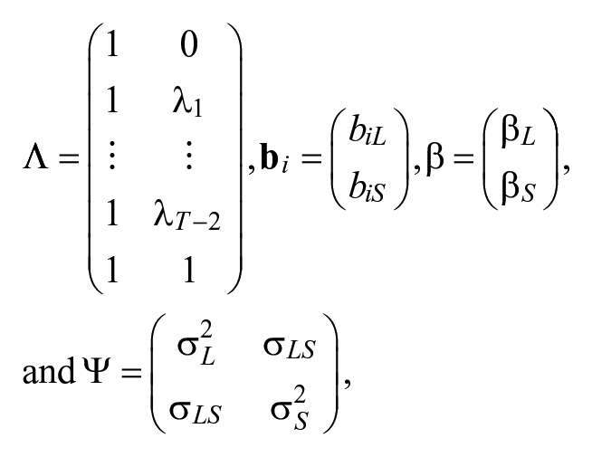
\begin{array}{l} Λ = (\begin{matrix} 1 & 0 \\ 1 & λ_{1} \\ ⋮ & ⋮ \\ 1 & λ_{T - 2} \\ 1 & 1 \end{matrix}), b_{i} = (\begin{matrix} b_{i L} \\ b_{i S} \end{matrix}), β = (\begin{matrix} β_{L} \\ β_{S} \end{matrix}), \\ and Ψ = (\begin{matrix} σ_{L}^{2} & σ_{L S} \\ σ_{L S} & σ_{S}^{2} \end{matrix}), \end{array}

the general latent growth curve models become LBGMs. In LBGMs, there are two latent factors, $b_{L}$ and $b_{S}$ , where $b_{L}$ represents the latent intercept and $b_{S}$ represents the total change over time. The first and the last factor loadings on $b_{S}$ are typically fixed to 0 and 1 as anchors, respectively, for identification purposes. All other factor loadings on $b_{S}$ are freely estimated. The parameters $λ_{1}, \dots, λ_{T - 2}$ are basis coefficients. They can determine the shape of the growth trajectories, and even the model specification. If $λ_{1}, \dots, λ_{T - 2}$ are equally spaced, the change in growth is linear, and the model becomes a linear growth curve model. Otherwise, if $λ_{1}, \dots, λ_{T - 2}$ are not equally spaced, the model is nonlinear. Figure 1 displays the path diagram of a LBGM as an example.

Figure 1.

Latent basis growth curve model with four measurement occasions.

We use Bayesian methods to estimate LBGMs. In the Bayesian framework, we rely on one single tool, the Bayes’s Theorem to obtain the joint posterior distributions of parameters based on the prior distributions and the data information. In the LBGMs, the joint probability distribution of $y_{i}, b_{i}$ is

\begin{array}{l} p (y_{i}, b_{i} | Φ, Λ, Ψ, β) = p (b_{i} | Ψ, β) p (y_{i} | b_{i}, Φ, Λ) \\ = {(2 π)}^{- \frac{m}{2}} {| Ψ |}^{- \frac{1}{2}} \exp [- \frac{1}{2} {(b_{i} - β)}^{'} Ψ^{- 1} (b_{i} - β)] \\ \times {(2 π)}^{- \frac{T}{2}} {| Φ |}^{- \frac{1}{2}} \exp [- \frac{1}{2} {(y_{i} - Λ b_{i})}^{'} Φ^{- 1} (y_{i} - Λ b_{i})] . \end{array}

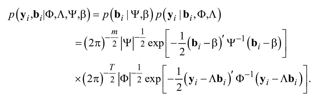
Thus, the likelihood function for the LBGM is

L = \prod_{i = 1}^{N} p (y_{i}, b_{i} | Φ, Λ, Ψ, β)

\begin{array}{l} \propto {| Ψ |}^{- \frac{N}{2}} \exp [- \frac{1}{2} \sum_{i = 1}^{N} {(b_{i} - β)}^{'} Ψ^{- 1} (b_{i} - β)] \\ \times {| Φ |}^{- \frac{N}{2}} \exp [- \frac{1}{2} \sum_{i = 1}^{N} {(y_{i} - Λ b_{i})}^{'} Φ^{- 1} (y_{i} - Λ b_{i})], \end{array}

where the unknown parameters in the LBGM include β, Λ, Φ, and ψ. Let $p (β, Λ, Φ, Ψ | y_{i})$ denote the joint prior distribution of these parameters. Thus, the joint posterior distribution is

p (β, Λ, Φ, Ψ | y_{i}) \propto \int p (β, Λ, Φ, Ψ) \times L d b .

Statistical inferences are usually difficult to be made directly from the joint posterior distributions. In Bayesian analysis with complex models, the conditional posterior distributions are relatively easy to obtain and can be used as a transition kernel to the joint distribution. Gibbs sampling, a MCMC algorithm, is often used to generate a sequence of samples from the joint probability distribution of two or more random variables (Casella & George, 1992). To be specific, Gibbs sampling alternately samples one parameter each time from its conditional posterior distribution conditional on the current values of the other parameters by treating the other parameters as known. After a sufficient number of iterations, the sequence of samples constitutes a Markov chain that converges to a stationary distribution. Geman and Geman (1984) showed that the stationary distribution of the Markov chain is actually the sought-after joint posterior distribution. Therefore, the Markov chain for model parameters or even augmented latent variables can be used to construct parameter estimates (Zhang et al., 2013). Gibbs sampling is especially useful when the joint probability distribution is too complex or unknown at all, but the conditional distribution for each parameter can be easily made available.

The Gibbs sampling algorithm is used to get parameter estimates for LBGMs. The detailed steps of the Gibbs sampling algorithm are given below.

Start with initial values $β^{(0)}, Ψ^{(0)}, Φ^{(0)}, {b_{i}}^{(0)}, Λ^{(0)},$ where $Λ = {(λ_{1}, \dots, λ_{T - 2})}^{'}$ .

Assume at the $j th$ iteration, we have $β^{(j)}, Ψ^{(j)}, Φ^{(j)}, b_{i}^{(j)}, Λ^{(j)}$ .

At the $(j + 1) th$ iteration,

3.1. Sample $β^{(j + 1)}$ from $p (β | Ψ^{(j)}, b_{i}^{(j)})$ ;

3.2. Sample $Ψ^{(j + 1)}$ from $p (Ψ | β^{(j + 1)}, b_{i}^{(j)})$ ;

3.3. Sample $Φ^{(j + 1)}$ from $p (Φ | Λ^{(j)}, b_{i}^{(j)}, y_{i})$ ;

3.4. Sample $b_{i}^{(j + 1)}, i = 1, \dots, N$ from p(b_i|Φ^(j+1), $Ψ^{(j + 1)}, β^{(j + 1)}, Λ^{(j)}, y_{i})$ ;

3.5. Sample $Λ^{(j + 1)}$ from $p (Λ b_{i}^{(j + 1)}, Φ^{(j + 1)}, y_{i})$ .

Repeat Step 3.

Bayesian Priors

In Bayesian statistical inference, prior of an uncertain quantity refers to one’s beliefs about this quantity before some evidence is taken into account. It can be knowledge gained previously such as background information or established theories, or even one’s intuitions. Often, the unknown quantity concerns parameters in a model. In this article, we believe model specification can also be viewed as an uncertain quantity. Although parameters in a model quantify characteristics of the population, the model specification reflects our beliefs of the structure of the data and it is at least as subjective as selecting a prior distribution for a model parameter. The rationale of incorporating model specification into the prior selection is that as both models and model parameters provide venues to understand the observed data and both model selection and parameter distribution selection are subjective, the source of information for Bayesian priors can be either from the model parameters or the models themselves.

There are two types of priors for the model parameters in the Bayesian framework: the noninformative priors and the informative priors. When previous knowledge is limited and priors are thus difficult to construct (Gill, 2014), noninformative priors are desirable to use. The rationale for using the noninformative priors is to “let the data speak for themselves” (Gelman et al., 2015, p. 51), such that the posterior distributions are dominated by the likelihood function, and the influence of prior information is minimized. In contrast, when researchers have a belief of the parameter distributions and use such information in model estimation, such prior knowledge is called informative prior, regardless of the sources of the information (e.g., a hypothesis being revised from theory, a pilot study or researchers’ intuitions; Gill, 2014; Muthen & Asparouhov, 2012). In latent growth curve modeling, it is likely that researchers are interested in the growth pattern of a psychological development or a cognitive ability, but they have no access to prior knowledge about it (e.g., no related study has been done previously). In this case, they may consider using noninformative priors. In practice, however, it is more likely that researchers have already had some prior knowledge about the parameters of interest in hand, and are doing further analysis of the data. For example, psychologists interested in learning participants’ change in attitude toward science may have had some expectations of the development in mind based on professional knowledge or empirical observations; educational researchers interested in studying children’s mathematical achievement may have learned previous academic growth from other published work (NICHD Early Child Care Research Network, 2007). These pieces of information are valuable to later research on understanding participants’ psychological development or academic growth, and they could serve as informative prior knowledge. With a strong belief and comprehensive prior knowledge, the informative prior of the development or growth could be accurate and precise. The informative prior distribution could also be “informative but weak,” as it is enough to keep posterior distribution within roughly reasonable bounds, but unable to capture the parameter knowledge (Gelman et al., 2015; Lambert, Sutton, Burton, Abrams, & Jones, 2005, p. 51). In such an instance, rather than a complete ignorance of knowledge, sometimes including even a small amount of information might be useful.

In LBGMs, prior selection for the basis coefficients adds an uncertainty in the parameter estimation. Specifically, different latent basis coefficients determine the shape of the growth trajectory and even the growth curve model. When priors of the latent basis coefficients are specified either incorrectly (i.e., the data are very different from what is expected from the prior) or with a lack of precision (i.e., prior distribution with a large variation), the posterior may be strongly influenced and the entire growth pattern may be distorted. Furthermore, selecting different priors for latent basis coefficients may lead to different models because the model specification can be viewed as being based on prior information. If the true growth pattern is nonlinear whereas latent basis coefficients are restricted to equally spaced values based on prior information, the LBGM becomes a linear growth curve model. Under this circumstance, model misspecification is a result of inaccurate prior selection and may greatly influence the parameter recovery and statistical inferences. In some sense, prior information can be divided into two layers. On the first layer, a model is specified based on researchers’ substantive theories or previous experiences. If there is no prior knowledge, a most general model is usually specified at the first step and this can be treated as a noninformative prior in model specification. On the second layer, given a specified model, priors are selected for model parameters. In the context of latent basis growth modeling, the two layers can be considered simultaneously. Consequently, the purpose of this study is to consider the two layers of prior selection procedure simultaneously in latent basis growth modeling, or in other words, to examine the impact of priors for model parameters as well as the impact of model misspecification on model estimation.

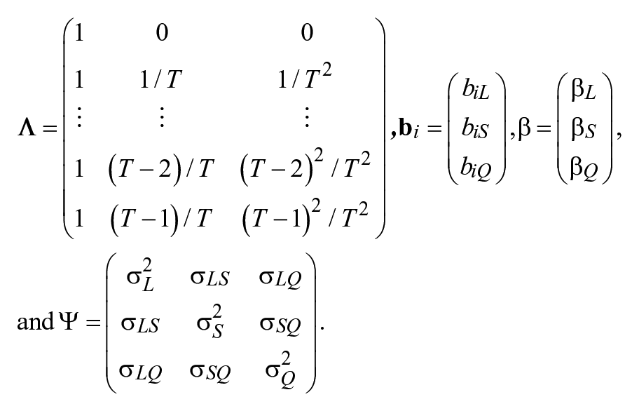
In this article, we evaluate the impact of priors for latent basis coefficients in LBGMs. For all the other model parameters, noninformative priors are applied. We consider four different types of priors for the latent basis coefficients to reflect commonly encountered situations in the real world. First, noninformative priors are used. In particular, we use diffuse priors as they are widely used noninformative priors that contain vague information with a large variance component to reflect “uncertainty in beliefs” (Kruschke, 2011, p. 39) or lack of knowledge in the prior information. Second, several sets of informative priors with different levels of accuracy and precision are investigated. It is rare but possible that researchers have a strong belief of very accurate knowledge about the parameters of interest before collecting data and conducting data analysis. Such prior information is very accurate and precise. In practice, it is more likely that researchers’ previous knowledge may be outdated or slightly biased, meaning that the prior knowledge is less accurate. If researchers have strong beliefs about such biased information, the prior is inaccurate yet with high precision. In some circumstances, researchers may get the prior knowledge based on the observed data and thus use data-dependent priors (DDPs). As its name suggests, DDPs are formulated based on the information obtained from the same data, such as having the parameters being approximated by a sample statistics (Serang, Zhang, Helm, Steele, & Grimm, 2015). Third, when researchers strongly believe that the latent bases are equally spaced, they may simply fit a linear growth curve model by constraining the latent basis coefficients to be some exact numbers. These priors actually lead to a model misspecification issue. Naturally, because specifying models can be treated as applying informative prior knowledge, we further study another type of nonlinear growth curve model—the quadratic growth curve model and evaluate how these types of prior information affect the latent growth modeling. A quadratic growth curve model is another special case of the general growth curve models. The matrix form of the parameters in quadratic growth curve models can be presented as

\begin{array}{l} Λ = (\begin{matrix} 1 & 0 & 0 \\ 1 & 1 / T & 1 / T^{2} \\ ⋮ & ⋮ & ⋮ \\ 1 & (T - 2) / T & {(T - 2)}^{2} / T^{2} \\ 1 & (T - 1) / T & {(T - 1)}^{2} / T^{2} \end{matrix}), b_{i} = (\begin{matrix} b_{i L} \\ b_{i S} \\ b_{i Q} \end{matrix}), β = (\begin{matrix} β_{L} \\ β_{S} \\ β_{Q} \end{matrix}), \\ a n d Ψ = (\begin{matrix} σ_{L}^{2} & σ_{L S} & σ_{L Q} \\ σ_{L S} & σ_{S}^{2} & σ_{S Q} \\ σ_{L Q} & σ_{S Q} & σ_{Q}^{2} \end{matrix}) . \end{array}

Evaluating the Impact of Priors Using a Monte Carlo Simulation Study

Study Design

In this section, we evaluate the impact of eight different sets of priors for the latent basis coefficients in latent basis growth modeling through a Monte Carlo simulation study. Because a pilot study showed that the number of measurement occasions does not affect the model estimation, we focus on a LBGM with four measurement occasions as shown in Figure 1. The population parameters of the LBGMs are given by

\begin{array}{l} Λ = (\begin{matrix} 1 & 0 \\ 1 & 0.1 \\ 1 & 0.3 \\ 1 & 1 \end{matrix}), β = (\begin{matrix} β_{L} \\ β_{S} \end{matrix}) = (\begin{matrix} 5 \\ 2.5 \end{matrix}), \\ and Ψ = (\begin{matrix} σ_{L}^{2} & σ_{L S} \\ σ_{L S} & σ_{S}^{2} \end{matrix}) = (\begin{matrix} 0.8 & σ_{L S} \\ σ_{L S} & 0.8 \end{matrix}) . \end{array}

We manipulate three factors to generate data, including sample size, covariance between the two latent variables $σ_{L S}$ , and variance of intraindividual measurement errors $σ_{e .}^{2}$ First, three sample size conditions are considered: N = 50, 200, and 500. Second, the covariance between the two latent variables $σ_{L S}$ is 0.5, −0.3, or 0, representing positively, negatively, or none correlated factor relation. Third, the variance of measurement errors $σ_{ϵ}^{2}$ is 0.7 or 0.26, reflecting either relatively large or small measurement error. Given the above values of covariance between the two latent variables and variance of measurement errors, reliability of the measure for the observed scores ranges between 0.50 and 0.91, which are commonly seen in practice. Our previous pilot studies showed that factor variances do not have much influence on the basis coefficients estimation, we constraint the factor variances $σ_{L}^{2} and σ_{S}^{2}$ both to be 0.8.

For each set of the simulated data, the impact of eight sets of priors (see Table 1) for the latent basis coefficients, which fall into the four types as discussed in the previous section, is studied and compared.

Table 1.

Prior Specification of Latent Basis Coefficients for Simulation.

Population basis coefficients	λ₁ = 0.1	λ₂ = 0.3
Prior distribution specification
	λ₁	λ₂
P1	N(0, 1,000, 000)	N(0, 1,000, 000)
P2	N(0.1, 0.01)	N(0.3, 0.01)
P3	N(0.2, 0.01)	N(0.4, 0.01)
P4	N(0.3, 0.01)	N(0.9, 0.01)
P5	N(0.3, 0.0001)	N(0.9, 0.0001)
P6	Data-dependent prior
	N( ${\hat{λ}}_{1 . M L}$ , $s e_{λ_{1} . M L}$ )	N( ${\hat{λ}}_{2 . M L}$ , $s e_{λ_{2} . M L}$ )
P7	Linear growth curve model
	N(1/3,0)	N(2/3,0)
P8	Quadratic growth curve model

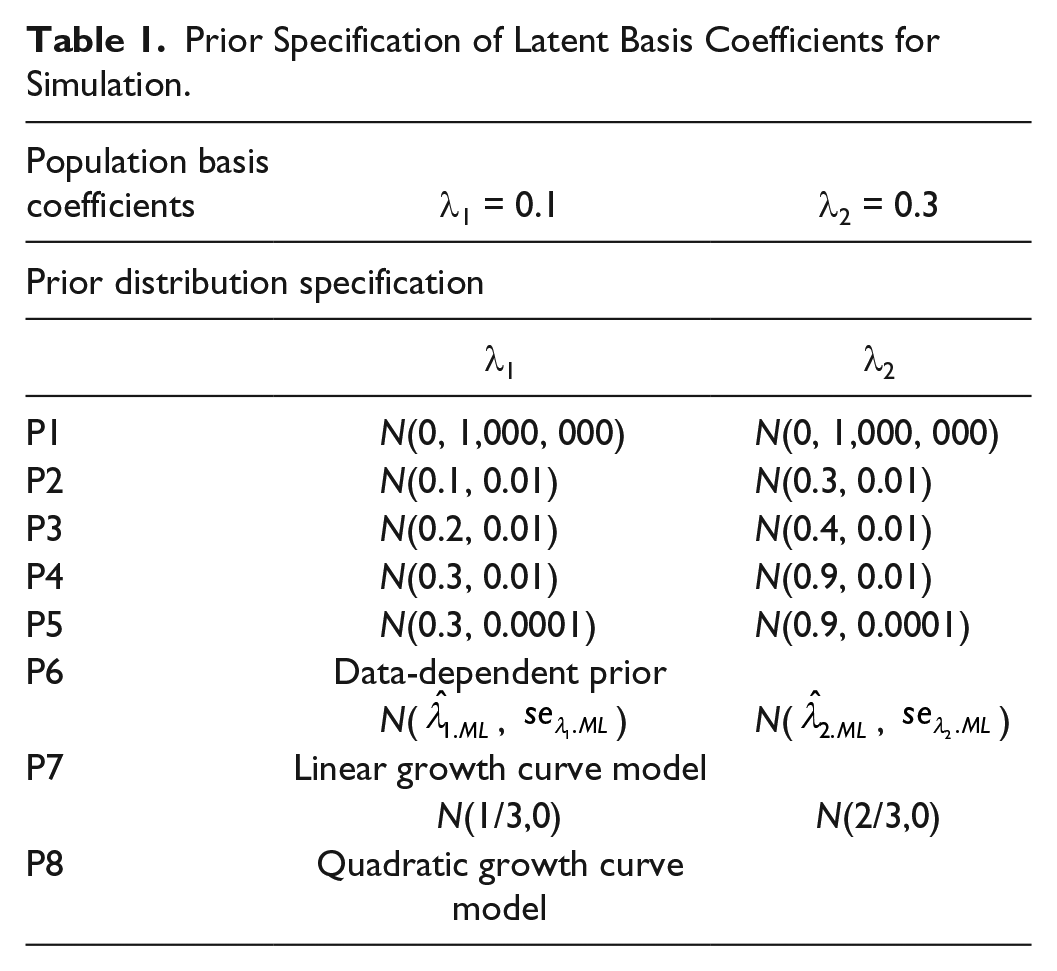
Priors P1 are noninformative priors. Priors P2 to P6 are informative priors. Particularly, priors P2 are the accurate informative prior as the priors reflect the actual parameter information. Priors P3 to P5 can be seen as the “weakly informative priors,” as information contained in these priors is not accurate but with a reasonable range of actual knowledge (Gelman, 2006). Priors P6 are also informative priors as they are data-dependent and gain information from the data. From priors P2 to P4, the accuracy of the priors reduces as the means of the priors deviate more from the true parameter values. Priors P5 have the same level of accuracy as priors P4 (both are inaccurate), but the distributions in P5 have smaller variances, meaning that we are more certain about the prior information in P5 than in P4 although the information is incorrect. Because DDPs are found to reduce bias in small samples in growth curve models (McNeish, 2016) and provide a possible alternative strategy to incorporate prior information when the information is limited, we also use DDPs as priors P6. For these priors, ML parameter estimates and the associated standard errors (SEs) are first obtained through the ML estimation of the model to the data, and the estimates and the associated SEs are then used as the hyperparameters in Bayesian prior specifications. When we have even stronger belief about the latent basis coefficients, the model specification may be influenced more. Priors P7 and P8 are used to illustrate this situation and are the remaining two types of priors for model specification. In P7, the latent basis coefficients are fixed at equally spaced values (λ₁ = 1/3 and λ₂ = 2/3), and thus the model becomes a linear growth curve model. We further study the effect of model misspecification and consider priors P8—specifying a quadratic growth curve model. In P8, the latent basis coefficients for $β_{S}$ are fixed to be $λ_{1} = 1 / 3 and λ_{2} = 2 / 3$ , and the basis coefficients for $β_{Q}$ are fixed to be $λ_{1}^{2} = 1 / 9 and λ_{2}^{2} = 4 / 9$ , so that the model becomes a quadratic curve model.

All the models are estimated using Bayesian methods. The simulation is conducted using R (R Development Core Team, 2011) and OpenBUGS (Thomas, O’Hara, Ligges, & Sturtz, 2006). An example of OpenBUGS script is provided in the appendix to facilitate the application of the Bayesian methods for latent basis growth modeling.

Evaluation criterion

The impact of the priors on model estimation is evaluated. First, for the LBGMs, we assess bias, SEs, and mean squared errors (MSEs) of the parameter estimates for the latent basis coefficients λ₁ and λ₂, as well as other model parameters. Let θ denote the population parameter value, and let $\hat{θ}$ _r, $r = 1, \dots, 500$ denote its estimate from the $r th$ simulation replication. The replication estimate is calculated as the average of parameter estimates more than 500 simulation replications.

Bias captures the distance between the replication estimate and its population parameter value,

b i a s = \frac{1}{500} \sum_{r = 1}^{500} {\hat{θ}}_{r} - θ .

SE is the standard deviation of the replication estimate, and MSE of the estimate is the expectation of its squared deviation from the true value.

M S E = E [{(\frac{1}{500} \sum_{r = 1}^{500} {\hat{θ}}_{r} - θ)}^{2}] .

Second, to compare the prior condition P7 where the model becomes a linear growth curve model with conditions P1 to P6, we study the estimates of the average latent intercept β_L and the average total change over time β_S, and compare them across conditions.

Third, the deviance information criterion (DIC; Spiegelhalter, Best, Carlin, & Linde, 2002) is used as a useful tool for Bayesian model assessment and model comparison. Similar to the model fit index BIC (Bayesian information criterion) from frequentist approach, DIC measures a combination of model complexity and model fit (e.g., Gill, 2014; Zhang et al., 2013). DIC is particularly useful in Bayesian model comparisons as the posterior distributions of the parameters have been obtained by MCMC simulations. Given the fact that the parameter estimates from the quadratic growth curve models cannot be directly compared with those from the other models, we use DIC to compare the quadratic growth curve models with the others and determine the best fitting models.

Results

Bias, SE, and MSE of the estimated basis coefficients $\hat{λ}$ ₁ and $\hat{λ}$ ₂ are presented in Tables 2 and 3, respectively. Because the parameter β_s, which represents the average total change over time, is the focus of the primary interest to developmental researchers (e.g., Jelicic, Phelps, & Lerner, 2009), we also present the bias, SE, and MSE of the parameter estimate $\hat{β}$ _S, as shown in Table 4.

Table 2.

VBias, SE, and MSE for the Latent Basis Coefficient λ₁.

$σ_{L S}$	N	Prior	$σ_{ϵ}^{2}$ = 0.7			$σ_{ϵ}^{2}$ = 0.26
$σ_{L S}$	N	Prior	Bias	SE	MSE	Bias	SE	MSE
0.5	50	P1	−0.002	0.061	0.004	−0.003	0.039	0.002
		P2	0.001	0.042	0.002	−0.002	0.033	0.001
		P3	0.034	0.041	0.003	0.014	0.033	0.001
		P4	0.093	0.040	0.010	0.044	0.032	0.003
		P5	0.199	0.001	0.040	0.198	0.001	0.039
		P6	0.015	0.175	0.031	0.000	0.076	0.006
	200	P1	−0.002	0.029	0.001	−0.001	0.018	0.000
		P2	−0.002	0.026	0.001	−0.001	0.018	0.000
		P3	0.010	0.026	0.001	0.004	0.017	0.000
		P4	0.031	0.025	0.002	0.013	0.017	0.000
		P5	0.195	0.001	0.038	0.192	0.002	0.037
		P6	−0.002	0.077	0.006	−0.004	0.037	0.001
	500	P1	−0.001	0.019	0.000	0.000	0.012	0.000
		P2	−0.001	0.018	0.000	0.000	0.012	0.000
		P3	0.004	0.018	0.000	0.002	0.012	0.000
		P4	0.014	0.018	0.001	0.006	0.012	0.000
		P5	0.188	0.002	0.035	0.179	0.002	0.032
		P6	0.001	0.056	0.003	−0.001	0.031	0.001
−0.3	50	P1	−0.008	0.064	0.004	−0.004	0.038	0.001
		P2	−0.002	0.043	0.002	−0.003	0.032	0.001
		P3	0.033	0.042	0.003	0.014	0.032	0.001
		P4	0.095	0.041	0.011	0.046	0.031	0.003
		P5	0.199	0.001	0.040	0.198	0.001	0.039
		P6	0.022	0.261	0.068	−0.010	0.096	0.009
	200	P1	−0.002	0.031	0.001	−0.003	0.019	0.000
		P2	−0.001	0.028	0.001	−0.002	0.018	0.000
		P3	0.011	0.027	0.001	0.002	0.018	0.000
		P4	0.033	0.027	0.002	0.011	0.018	0.000
		P5	0.196	0.001	0.038	0.193	0.001	0.037
		P6	−0.013	0.110	0.012	−0.007	0.043	0.002
	500	P1	0.000	0.020	0.000	0.001	0.012	0.000
		P2	0.000	0.019	0.000	0.001	0.012	0.000
		P3	0.005	0.019	0.000	0.003	0.012	0.000
		P4	0.015	0.019	0.001	0.006	0.012	0.000
		P5	0.189	0.002	0.036	0.182	0.002	0.033
		P6	−0.010	0.063	0.004	−0.003	0.032	0.001

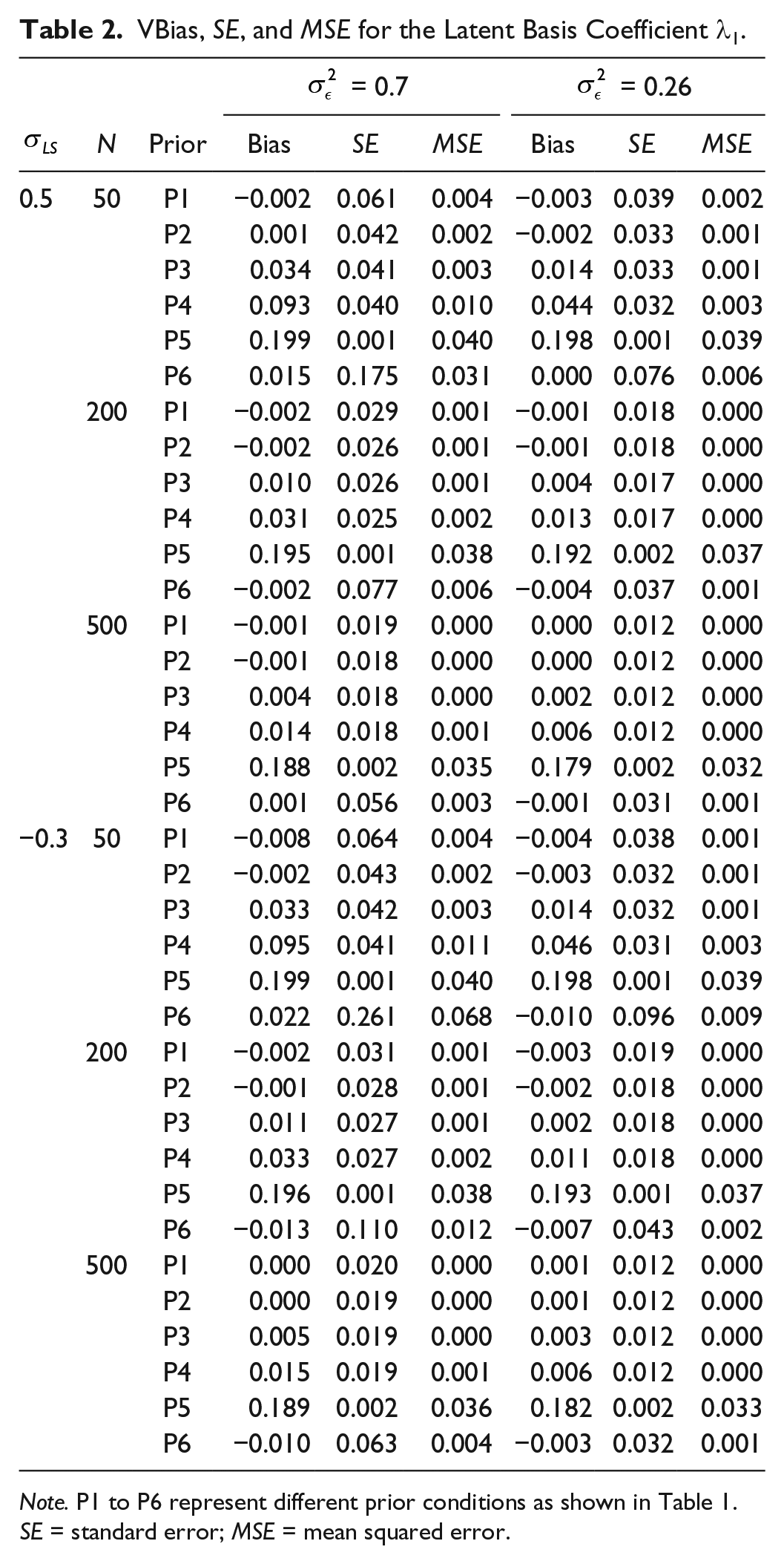
Note. P1 to P6 represent different prior conditions as shown in Table 1. SE = standard error; MSE = mean squared error.

Table 3.

Bias, SE, and MSE for the Latent Basis Coefficient λ₂.

$σ_{L S}$	N	Prior	$σ_{ϵ}^{2}$ = 0.7			$σ_{ϵ}^{2}$ = 0.26
$σ_{L S}$	N	Prior	Bias	SE	MSE	Bias	SE	MSE
0.5	50	P1	−0.001	0.058	0.003	−0.001	0.034	0.001
		P2	0.001	0.042	0.002	0.000	0.030	0.001
		P3	0.032	0.042	0.003	0.014	0.029	0.001
		P4	0.162	0.045	0.028	0.071	0.030	0.006
		P5	0.593	0.001	0.352	0.589	0.001	0.347
		P6	0.024	0.181	0.033	0.008	0.083	0.007
	200	P1	−0.001	0.031	0.001	0.000	0.017	0.000
		P2	0.000	0.028	0.001	0.000	0.016	0.000
		P3	0.010	0.028	0.001	0.004	0.016	0.000
		P4	0.049	0.027	0.003	0.020	0.016	0.001
		P5	0.572	0.002	0.327	0.554	0.002	0.307
		P6	0.010	0.083	0.007	−0.002	0.039	0.002
	500	P1	0.000	0.018	0.000	0.001	0.011	0.000
		P2	0.000	0.018	0.000	0.001	0.011	0.000
		P3	0.004	0.018	0.000	0.003	0.011	0.000
		P4	0.021	0.017	0.001	0.009	0.011	0.000
		P5	0.528	0.003	0.278	0.472	0.004	0.223
		P6	−0.002	0.052	0.003	0.002	0.029	0.000
−0.3	50	P1	−0.004	0.058	0.003	−0.003	0.037	0.001
		P2	−0.001	0.041	0.002	−0.002	0.032	0.001
		P3	0.032	0.040	0.003	0.013	0.032	0.001
		P4	0.172	0.045	0.032	0.074	0.034	0.007
		P5	0.594	0.001	0.352	0.590	0.001	0.348
		P6	0.037	0.253	0.066	0.007	0.101	0.010
	200	P1	−0.001	0.028	0.001	−0.001	0.018	0.000
		P2	−0.001	0.025	0.001	−0.001	0.018	0.000
		P3	0.010	0.025	0.001	0.003	0.018	0.000
		P4	0.051	0.025	0.003	0.019	0.017	0.001
		P5	0.575	0.002	0.330	0.560	0.002	0.314
		P6	0.020	0.112	0.013	−0.001	0.045	0.002
	500	P1	0.001	0.018	0.000	0.001	0.010	0.000
		P2	0.001	0.018	0.000	0.001	0.010	0.000
		P3	0.005	0.018	0.000	0.003	0.010	0.000
		P4	0.023	0.017	0.001	0.009	0.010	0.000
		P5	0.536	0.003	0.287	0.494	0.004	0.244
		P6	0.001	0.059	0.003	0.000	0.030	0.001

Note. P1 to P6 represent different prior conditions as shown in Table 1. SE = standard error; MSE = mean squared error.

Table 4.

Bias, SE, and MSE for the Parameter β_S.

$σ_{L S}$	N	Prior	$σ_{ϵ}^{2}$ = 0.7			$σ_{ϵ}^{2}$ = 0.26
$σ_{L S}$	N	Prior	Bias	SE	MSE	Bias	SE	MSE
0.5	50	P1	−0.028	0.208	0.044	0.006	0.154	0.024
		P2	−0.019	0.201	0.041	0.008	0.152	0.023
		P3	0.017	0.200	0.040	0.026	0.151	0.024
		P4	0.031	0.210	0.045	0.055	0.151	0.026
		P5	−0.576	0.173	0.361	−0.548	0.126	0.316
		P6	0.007	0.219	0.048	−0.001	0.168	0.028
		P7	−0.118	0.198	0.053	−0.092	0.147	0.030
	200	P1	0.000	0.102	0.010	−0.002	0.081	0.007
		P2	0.001	0.101	0.010	−0.002	0.081	0.007
		P3	0.014	0.100	0.010	0.004	0.081	0.007
		P4	0.038	0.099	0.011	0.015	0.081	0.007
		P5	−0.520	0.091	0.279	−0.487	0.069	0.242
		P6	−0.005	0.110	0.012	−0.002	0.085	0.007
		P7	−0.096	0.099	0.019	−0.102	0.077	0.016
	500	P1	−0.006	0.063	0.004	−0.003	0.053	0.003
		P2	−0.005	0.063	0.004	−0.003	0.053	0.003
		P3	0.000	0.063	0.004	−0.001	0.053	0.003
		P4	0.013	0.062	0.004	0.004	0.053	0.003
		P5	−0.439	0.059	0.196	−0.329	0.053	0.111
		P6	−0.006	0.071	0.005	0.001	0.054	0.003
		P7	−0.094	0.060	0.013	−0.096	0.050	0.012
−0.3	50	P1	−0.034	0.202	0.042	−0.013	0.158	0.025
		P2	−0.022	0.194	0.038	−0.011	0.156	0.024
		P3	0.017	0.193	0.038	0.008	0.155	0.024
		P4	0.027	0.204	0.042	0.038	0.155	0.026
		P5	−0.574	0.168	0.358	−0.564	0.131	0.335
		P6	0.021	0.213	0.046	0.031	0.167	0.029
		P7	−0.111	0.192	0.049	−0.105	0.152	0.034
	200	P1	−0.003	0.104	0.011	0.002	0.084	0.007
		P2	−0.002	0.103	0.011	0.002	0.084	0.007
		P3	0.012	0.102	0.011	0.008	0.084	0.007
		P4	0.037	0.102	0.012	0.019	0.083	0.007
		P5	−0.525	0.092	0.284	−0.494	0.074	0.249
		P6	0.008	0.108	0.012	0.006	0.084	0.007
		P7	−0.096	0.101	0.019	−0.095	0.081	0.016
	500	P1	−0.007	0.061	0.004	−0.002	0.054	0.003
		P2	−0.007	0.060	0.004	−0.002	0.054	0.003
		P3	−0.001	0.060	0.004	0.000	0.054	0.003
		P4	0.012	0.060	0.004	0.005	0.054	0.003
		P5	−0.459	0.058	0.214	−0.372	0.052	0.141
		P6	−0.002	0.071	0.005	−0.006	0.054	0.003
		P7	−0.099	0.059	0.013	−0.098	0.051	0.012

Note. P1 to P7 represent different prior conditions as shown in Table 1. SE = standard error; MSE = mean squared error.

The estimates for other model parameters are available upon request, but not given in this section to save space. To evaluate the impact of priors which resulted in model specification, DICs for the misspecified models are compared with those for latent basis models with noninformative priors and accurate informative priors.

Overall, as sample size increases, parameter estimates have decreased bias and SEs, and the impact of prior specifications on the parameter estimation decreases. The covariance between the two latent variables, $σ_{L S}$ , does not have a salient influence on the model estimation across different prior conditions. In this section, we present the results for parameter estimates when the covariance between the two latent variables is nonzero to save space. In addition, smaller variance of intraindividual measurement errors $σ_{ϵ}^{2}$ leads to less biased parameter estimates and smaller SEs, and this pattern stays the same throughout all the prior specifications for LBGMs except for priors P5. For example, for priors P4, with the prior means far away from the true parameter values, $σ_{ϵ}^{2}$ affects the performance of the parameter estimates in regard to accuracy and efficiency. However, the estimation performance is not affected as much when priors P5 are specified because the precision of the priors P5 is very high. These patterns are shown in Tables 2 and 3.

We take a close look at the impact of different priors on model estimation. Prior specifications on the latent basis coefficients affect the parameter estimates for LBGMs. Among all the prior specifications, priors P2 lead to the smallest MSE, showing that accurate informative priors P2 lead to the most accurate and efficient combination of parameter estimates across all conditions.

Comparing the performance of all the informative priors in the basis coefficients estimation, the benefit of using priors P2 over other informative priors is especially obvious when sample size is small. For example, when sample size is 50, $σ_{ϵ}^{2}$ = 0.7 and $σ_{L S}$ = −0.3, the bias of $λ$ ₁ estimate for priors P2 is −0.002, much smaller than the estimation bias from other informative prior specifications. Specifying priors P3 where the prior knowledge is away from the true information results in more biased basis coefficient estimates but similar SEs when being compared with those from the P2 condition. When priors P4 or P5 are specified, regardless of other data conditions, the parameter estimates are unacceptably different from the true parameter values. Although specifying priors P5 produces the smallest SE estimates, the estimates in the meantime are severely biased due to the low accuracy in priors P5.

For DDP priors P6, nonconvergence occurs in ML estimation for the basis coefficients especially when sample size is small, and only converged results are reported. Comparing the performance of priors P6 to the performance of other informative priors, although DDP priors P6 performs slightly worse than the accurate informative priors P2, they produce relatively smaller bias than other inaccurate informative priors P3 to P5. For example, when N = 200, $σ_{L S} = 0.5, σ_{ϵ}^{2} = 0.7,$ the bias from P6 is −0.002, whereas the bias from P3 to P5 are 0.010, 0.031, 0.195, much larger in magnitude. However, using DDP priors P6 also brings in relatively larger SEs across all data conditions. This is probably because ML estimates based on the data in the first step may vary from sample to sample, which directly affects the prior specifications in the second step and causes large SEs across conditions. Nevertheless, as a combination of bias and SEs, the MSEs produced by priors P6 are reasonable. For example, when N = 500, $σ_{L S} = - 0.3, σ_{ϵ}^{2} = 0.26$ , although the SE is as large as 0.032, the bias is small and thus the MSE is relatively small as 0.001. This shows that using DDP priors P6 has the advantage of producing relative accurate basis coefficient estimates especially in small samples, and can be considered to be used when limited background information is available.

Comparing the performance of the informative priors with that of the noninformative priors P1, using priors P1 and priors P2, lead to very similar results in terms of bias. For example, when sample size is 50, $σ_{ϵ}^{2}$ = 0.7 and $σ_{LS}$ = −0.3, the bias of $λ$ ₂ estimate for priors P2 is −0.001. Although the bias based on priors P1 is −0.004, four times larger in magnitude than the bias for priors P2, the difference is tiny in magnitude. However, priors P2 produce more efficient basis coefficient estimates than priors P1 do when sample size is small. The advantage of larger efficiency in priors P2 over priors P1 wanes as sample size increases. This is because as more information from data comes in, the influence of the likelihood increases and the influence of the prior on the posterior diminishes. Although the merit of using accurate informative priors over noninformative priors seems trivial, the advantage of using accurate informative priors is obvious in terms of statistical power. For example, simulation results show that when N = 200, $σ_{ϵ}^{2}$ = 0.7, and $σ_{L S}$ = 0.5, the statistical power increased from .43 when priors P1 are specified to .56 when priors P2 are specified.

As shown in Table 4, when priors P7 are applied, in other words, when we believe that the growth pattern is linear and fit a linear growth curve model to the data whereas the true model is nonlinear, the model parameter estimates are biased. The bias under P7 conditions is much larger than those under prior conditions P1 to P6, although priors P4 are inaccurate priors with small precisions. Therefore, we conclude that prior information which results in model misspecification can largely influence the model estimation and interpretations.

As discussed previously, model specification can be treated as a prior selection process, and we use DIC to evaluate the impact of such prior information. Table 5 presents average DICs across all replications under prior conditions P1, P2, P7, and P8. Corresponding DICs under prior conditions P3 to P6 are relatively larger than those under prior conditions P1 and P2, and thus are omitted here. The result shows that DICs for the LBGM with noninformative priors P1 and accurate informative priors P2 are comparable. Although DICs are smaller when priors P2 are used, the difference is almost negligible, especially when sample size is large and the intraindividual measurement error is small. For example, in conditions where no correlation between the latent intercept and slope is present, when $σ_{ϵ}^{2}$ = 0.26 and sample size is 500, the DIC for latent basis model with priors P1 is 4,972.598 and with priors P2 is 4,972.326. DIC is better to be used to compare different priors when the prior information leads us to fit different models to the data. When the quadratic growth curve model is fitted to the data, in other words, when priors P8 are applied, DICs are much larger, indicating that such prior information has a big adverse impact on the model estimation. When the linear growth curve model is fitted to the data, in other words, when priors P7 are applied, there are circumstances that DICs for priors P7 are smaller than those for priors P1 and P2, when measurement error is large (e.g., $σ_{ϵ}^{2} = 0.7)$ . This is probably because with more intraindividual measurement errors being included, the nonlinear growth pattern could be hidden as if the pattern was linear, and DIC selects a simple model. When measurement error is relatively small (e.g., $σ_{ϵ}^{2} = 0.26$ ), DICs are larger than those with priors P1 and P2, meaning that linear growth curve models do not fit the data well.

Table 5.

DIC for Models With Priors P1, P2, P7, and P8.

N	Prior	$σ_{L S}$ = 0.5		$σ_{L S}$ = 0		$σ_{L S}$ = −0.3
N	Prior	$σ_{ϵ}^{2}$ = 0.7	$σ_{ϵ}^{2}$ = 0.26	$σ_{ϵ}^{2}$ = 0.7	$σ_{ϵ}^{2}$ = 0.26	$σ_{ϵ}^{2}$ = 0.7	$σ_{ϵ}^{2}$ = 0.26
50	P1	638.364	477.792	690.680	534.961	698.931	537.665
	P2	636.154	476.372	688.158	532.705	696.226	535.265
	P7	652.622	532.694	677.042	570.144	680.627	582.445
	P8	650.991	506.126	695.217	570.678	699.870	572.320
200	P1	2,597.098	1,959.536	2,829.876	2,034.031	2,856.435	2,031.256
	P2	2,596.222	1,958.957	2,828.200	2,033.300	2,854.585	2,030.537
	P7	2,577.063	2,087.639	2,704.513	2,271.868	2,742.923	2,341.444
	P8	2,677.863	2,106.722	2,905.419	2,262.603	2,933.759	2,240.978
500	P1	6,610.351	4,899.720	6,968.144	4,972.598	6,980.828	4,969.590
	P2	6,609.874	4,899.464	6,967.314	4,972.326	6,979.914	4,969.298
	P7	6,422.014	5,197.114	6,749.414	5,713.117	6,879.553	5,909.157
	P8	6,797.770	5,379.518	7,367.665	5,541.447	7,323.761	5,543.469

Note. DIC = deviance information criterion.

Example

A subset of the National Longitudinal Survey of Youth data from the 1979 cohort is used to illustrate that different prior specifications on the latent basis coefficients affect the model estimation and the interpretation of the growth pattern in latent basis growth modeling. Fifty schoolchildren’s Peabody Individual Achievement Test (PIAT) reading recognition was measured biyearly in 1986, 1988, 1990, and 1992. Figure 2 shows a trajectory plot of the data, with the red line representing the average score at each measurement occasion. The overall trajectory seems nonlinear. Given the prior knowledge that Zhang et al. (2007) fitted a LBGM to PIAT reading scores collected from the same cohort and the model fitted their data well, we use a LBGM (Figure 1) to analyze our data. In the latent basis growth modeling, we specify different priors for the latent basis coefficients and use noninformative priors for the remaining parameters. For illustration purposes, we compare four prior conditions. First, noninformative priors are applied, where both λ₁ and λ₂ follow a normal distribution N (0, 106).

Figure 2.

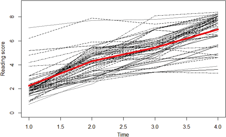
Longitudinal trajectory plot of PIAT reading data.

Second, based on the results from Zhang et al. (2007), informative priors λ₁ ∼ N (0.5, 0.01) and λ₂ ∼ N (0.8, 0.01) are used. Because Zhang et al. analyzed data from the same cohort, we assume their results can be trusted and treat this set of priors as accurate informative priors. Third, by fixing λ₁ at 1/3 and λ₂ at 2/3, the LBGM becomes a linear growth curve model, which is widely used in practice as it is easier to estimate and interpret. Because the trajectory plot suggests a nonlinear growth pattern, we treat this set of priors as inaccurate informative priors. In addition, we also fit a quadratic growth curve model to the data for comparison. As discussed previously, model specification can be also viewed as a way of prior selection. Thus, we compare four prior conditions in total.

The DICs for the linear growth model and quadratic growth model are 458.5 and 438.7, respectively. Both are much larger than the DICs for the LBGMs (DIC = 414.8 when the noninformative priors are used, DIC = 422.8 when the accurate informative priors are used, and DIC = 411.4 when the DDP are used), meaning that the LBGMs fit data better than the linear growth model and the quadratic growth model. Thus, we only compare the parameter estimates for the LBGMs with noninformative priors, accurate informative priors, and DDP. The results are provided in Table 6. The first two sets of priors lead to slightly different parameter estimates. The SEs of the estimates from the latent basis model with accurate informative priors are uniformly smaller than those from the latent basis model with noninformative priors, indicating that the accurate informative priors result in more precise parameter estimates. The DDP produces similar results to those from noninformative priors, and thus is an alternative strategy to be considered as a type of informative prior.

Table 6.

Parameter Estimates for PIAT Reading Data.

Prior	Parameter	Estimate	SE	CI lower	CI upper
Noninformative	λ₁	0.434	0.019	0.397	0.472
	λ₂	0.674	0.019	0.637	0.713
	β_L	2.252	0.191	1.889	2.629
	β_S	4.709	0.262	4.203	5.215
	σ_LS	1.581	0.378	0.943	2.360
	$σ_{ϵ}^{2}$	0.297	0.044	0.215	0.384
	$σ_{L}^{2}$	1.581	0.378	0.943	2.360
	$σ_{S}^{2}$	2.902	0.717	1.621	4.334
Accurate	λ₁	0.460	0.017	0.426	0.492
	λ₂	0.714	0.018	0.679	0.748
	β_L	2.195	0.191	1.818	2.561
	β_S	4.672	0.259	4.167	5.167
	σ_LS	1.590	0.383	0.934	2.372
	$σ_{ϵ}^{2}$	0.311	0.048	0.223	0.404
	$σ_{L}^{2}$	1.590	0.383	0.934	2.372
	$σ_{S}^{2}$	2.807	0.703	1.537	4.197
Data dependent	λ₁	0.434	0.013	0.409	0.459
	λ₂	0.674	0.013	0.648	0.701
	β_L	2.258	0.194	1.876	2.644
	β_S	4.702	0.268	4.177	5.228
	σ_LS	1.379	0.445	0.607	2.252
	$σ_{ϵ}^{2}$	0.293	0.043	0.220	0.388
	$σ_{L}^{2}$	1.582	0.378	0.990	2.469
	$σ_{S}^{2}$	2.919	0.728	1.755	4.597

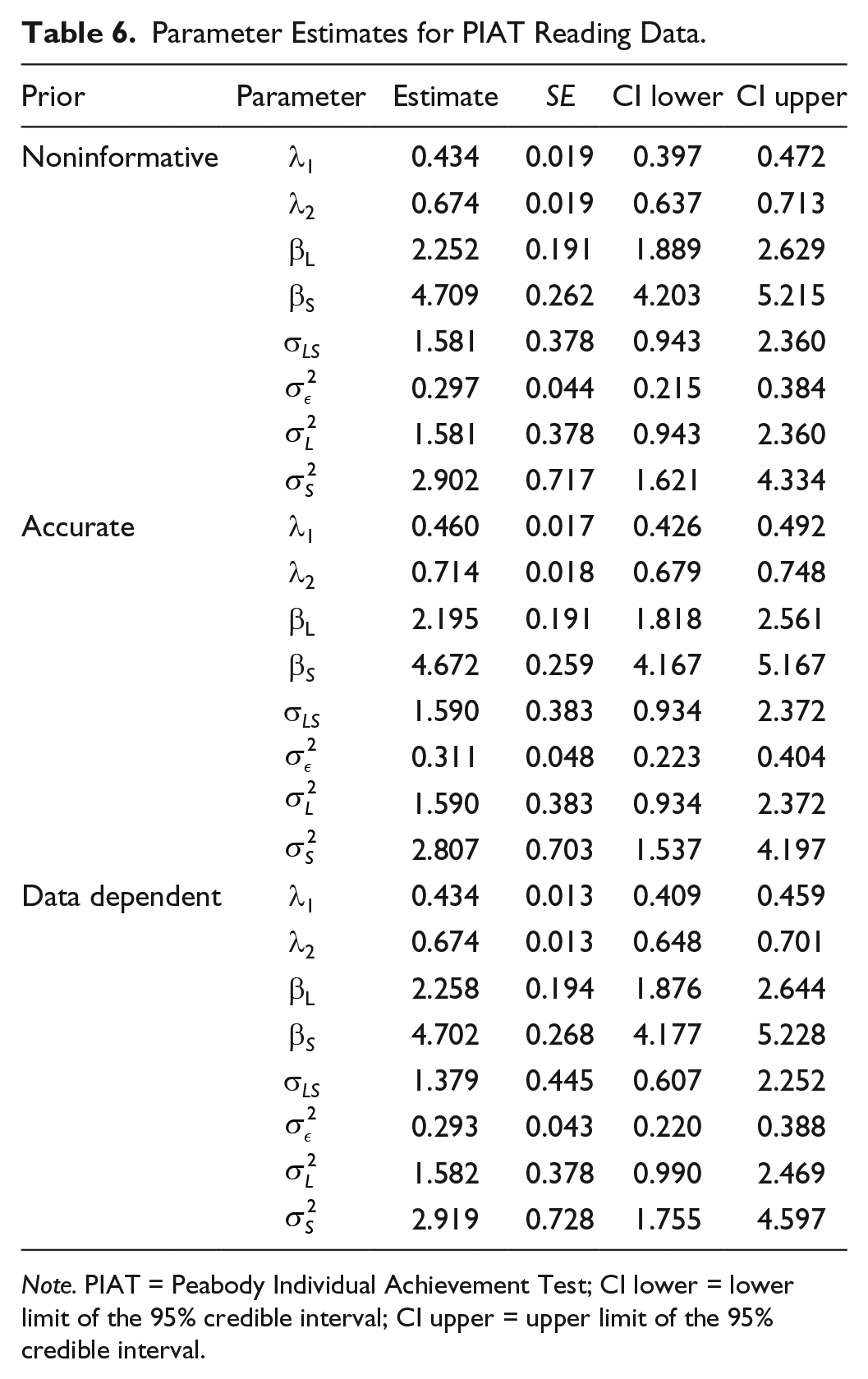
Note. PIAT = Peabody Individual Achievement Test; CI lower = lower limit of the 95% credible interval; CI upper = upper limit of the 95% credible interval.

Based on the simulation results discussed previously, we rely on the results from the LBGM with accurate informative priors because the sample size is relatively small in this example. The estimated basis coefficients show that the growth pattern of the reading scores is curvature rather than linear. The increase of schoolchildren’s reading scores was relatively faster at the beginning and slowed down at the later period of time. The average initial reading score is 2.195, and the average total change from 1986 to 1992 is 4.672. There are interindividual differences at both the initial values and the total changes over time, and the initial reading scores are positively correlated with the total change scores over time.

Discussion

In this study, the impact of two layers of prior information on the Bayesian estimation of LBGMs was investigated through a simulation study. In particular, eight sets of prior information with different levels of accuracy and precision were considered. Among the eight sets of priors, two are misspecified models: linear and quadratic growth curve models. We treated model misspecification as a special case of applying inaccurate informative priors and studied the impact of the model misspecification on the LBGM estimation. Three potentially influential factors were considered, including covariance between the two latent variables, variance of intraindividual measurement errors, and sample size. Based on the simulation results, following conclusions are drawn.

Overall, sample size affects the Bayesian estimation of latent basis coefficients. As sample size increases, the impact of prior information decreases and the posterior parameter estimation is more affected by the observed data. When sample size is extremely large, the prior is said to be “swamped by the data” (see, for example, Bolstad, 2007; Muthen & Asparouhov, 2012; Scheines et al., 1999). Then, under different prior specifications, intraindividual measurement errors have an influence on the parameter estimates. Small measurement errors yield relatively more accurate and efficient basis coefficient estimates, even when the priors are inaccurate. This is probably because with small measurement errors, the observed sample data have explained the majority of the variance of accuracy in basis coefficients, which in turn reduces the influence of the prior information. In addition, the covariance between the two latent variables has no apparent influence on the parameter estimates.

Specifying priors on the latent basis coefficients does not only affect basis coefficients estimates but also has an impact on the performance of the other model parameter estimates, including the average latent intercept and the average total change over time. Therefore, even the growth pattern may be misinterpreted when inaccurate priors are applied, let alone the interpretations for interindividual differences and the relationship between the initial values and the total change scores. When previous information leads to misspecified models, DIC can be used to detect the inaccurate prior information. For example, DIC shows strong model misfit in the simulation study as the true growth pattern is nonlinear whereas we fit a linear growth model to the data. Therefore, as we never know whether previous information is accurate or not, a linear relationship should be specified with caution as potential problems of model misfit might arise and result in misleading interpretations. A LBGM is more general and thus recommended to use.

In Bayesian methods, prior selection is important for latent basis growth modeling, as prior information affects the model parameter estimates and thus the shape of the latent growth trajectories. Theoretically, when one is certain about previous knowledge and the previous knowledge is correct, such informative priors produce the most accurate and efficient parameter estimates. Limited and inaccurate previous knowledge is very likely to lead to inefficient or even incorrect parameter estimates. Although the performance of the noninformative priors and the accurate informative priors seems similar in terms of bias and SEs, accurate informative priors P2 bring in a substantive increase in statistical power compared with noninformative priors P1 under some circumstances. Note that the positive impact of noninformative priors in the context of LBGMs runs differently from that in the growth mixture modeling context, where research on the latter concluded that the noninformative priors on the specification of mixture proportions in the growth mixture model had a harmful impact and recommended against using noninformative priors under any conditions (e.g., Roeder & Wasserman, 1997).

In practice, it is impossible to know whether previous knowledge is accurate or not. Thus, we recommend doing more empirical research and obtain a comprehensive understanding of the substantive interest before making prior selection decisions. It is always a sound scientific practice to do more research in the substantive model to seek for accurate information. However, if prior knowledge is not easily accessible, or even no information is available at all, or previous studies had contradictory conclusions, several remedial strategies may be considered. First, if sample size is reasonably large, one may use noninformative priors in Bayesian estimation to “let the data speak for themselves” (Gelman et al., 2015). However, using noninformative priors should only be seen as a “provisional” strategy and the posterior distribution should always be examined after the model is fitted (Gelman, 2006). If the posterior distribution contradicts previous knowledge or the assumptions of prior distributions, one should always look for additional prior information and fine-tune prior distributions accordingly. Second, when sample size is small and researchers are not confident about the previous knowledge they obtained, we suggest comparing the estimation results based on some informative priors as well as those based on noninformative priors. If the results differ dramatically, further research is needed to obtain more information or additional data need to be collected. Empirically, the DDPs may be adopted as they combine the information from the data using frequentist method and take advantage of the Bayesian method for the estimation. Last, as the model misspecifications adversely affect the model estimations, when limited information about the data structure is available and the choice of the model specification is unclear, a more flexible version of the growth curve model, the LBGM is recommended to be used.

In Bayesian analysis, priors are usually selected for model parameters, but in this article, we treated the model specification as a prior selection procedure as well. Model misspecification is treated as if we had applied inaccurate prior information to the data analysis. This type of inaccurate priors affects the model estimation the most. For example, when a linear growth trajectory is incorrectly specified given the true growth pattern is nonlinear, the estimated growth pattern could be distorted. In addition to LBGMs, the idea of viewing model specification as a prior selection procedure can be extended to other models. For example, in confirmatory factor models with cross loadings, misspecifying models by omitting cross loadings can be viewed as a procedure of selecting wrong priors (Shi & Tong, 2016). This type of prior information should be carefully applied as it may substantially affect model estimation, and may result in misleading interpretation. For confirmatory factor analysis, Bayesian ridge regression priors (Muthen & Asparouhov, 2012) and spike-and-slab priors (Lu, Chow, & Loken, 2016) have been used as variable selection tools. The same ideas can be applied to latent basis growth modeling as well.

We would like to note that although Bayesian statistics has been criticized for its “subjectivity” in assigning prior distributions to model parameters, the model specification itself is subjective regardless of the choice of Bayesian or frequentist approach. For example, in a longitudinal study of child development where the underlying growth trajectory is nonlinear, the first step of selecting a linear growth curve model to fit the data is subjective and may be misleading. This study shows that the model misspecification adversely affects the parameter estimation much more than selecting inaccurate prior distributions. Therefore, the subjectivity of specifying a prior for model parameters in Bayesian method is no more serious than specifying a model. Bayesian approach is more flexible in considering the uncertainty in the model specification.

Footnotes

Appendix

An OpenBUGS script for the latent basis growth model with accurate informative priors in the simulation study.

Model {

for ( i i n 1 :N) {

LS [ i, 1 : 2 ] ~ dmnorm ( muLS [ i, 1 : 2 ], inv_cov [ 1 : 2, 1:2]) muLS [ i,1] < −bL [ 1 ]

muLS [ i,2] < − bS [ 1 ]

for ( t i n 1 : 4 ) {

y [ i, t ]~ dnorm (muY[ i, t ], inv_sig_e2 ) muY[ i, t ]<−LS [ i,1]+ LS [ i, 2 ] * A[ t ]

}

## Priors for the latent intercept and the total change over time for ( i i n 1 : 1 ) {

bL [ i ]~ dnorm ( 0, 1 . 0 E−6) # diffuse bS [ i ]~ dnorm ( 0, 1 . 0 E−6) # diffuse

}

## Priors for the latent basis coefficients

A[1] < −0

A[ 2 ] ~ dnorm ( . 1, 1 . 0 E+ 2 ) ## accurate informative A[ 3 ] ~ dnorm ( . 3, 1 . 0 E+ 2 ) ## accurate informative

A[4] < −1

## Priors for the covariance between the intercept and the total change over time inv_cov [ 1 : 2, 1 : 2 ] ~ dwish (R [ 1 : 2, 1 : 2 ], 2 ) # d i f fuse

R[1,1] < −1

R[2,2] < −1

R[2,1] < −R[ 1,2] R[1,2] < −0

## Priors for the residual variance

i n v _ s i g _ e 2 ~dgamma ( . 0 0 1, . 001) # d i ffuse sig_e2 <−1/ inv_sig_e2

cov [1:2, 1:2] < − inverse ( inv_cov [ 1 : 2, 1:2])

## Priors for the variance of the latent intercept and the variance of the total change over time sig_L2 <−cov [ 1, 1 ]

sig_S2 <−cov [ 2, 2 ] cov_LS<−cov [ 1, 2 ]

rho_LS<−cov [1,2]/ sqrt ( cov [ 1, 1 ] * cov [2,2])

## Summarize the parameters into a vector

parm [1]< −A[ 2 ] # basis coefficients

parm [2]< −A[ 3 ] # basis coefficients

parm [3]< −bL [ 1 ] # mean of latent intercept

parm [4]< − bS [ 1 ] # mean of total change over time

parm [5]< − cov [ 1 : 2, 1 : 2 ] # covariance between latent intercept and the total change over time

parm [6]< − sig_e2 # residual variance

parm [7]< − s ig_ L 2 # variance of the latent intercept

parm [8]< − s i g _ S 2 # variance of the total change over time

}

Declaration of Conflicting Interests

The author(s) declared no potential conflicts of interest with respect to the research, authorship, and/or publication of this article.

Funding

The author(s) received no financial support for the research, authorship, and/or publication of this article.

Author Biographies

Dingjing Shi is a PhD student in the Department of Psychology at the University of Virginia. Dingjing is interested in developing and applying statistical methods to psychology and other social and behavioral science fields. Dingjing’s research interests include latent variable modeling, longitudinal data analysis, Bayesian methods and missing data.

Xin Tong is an assistant professor in the Department of Psychology at the University of Virginia. Xin’s research focuses on developing and applying statistical methods in the areas of developmental and health studies. Methodologically, Xin is interested in Bayesian methodology, growth curve modeling, and robust structural equation modeling with nonnormal and missing data.

References

Bolstad

(2007). Introduction to Bayesian statistics (2nd ed.). New York, NY: John Wiley.

Casella

Berger

R. L.

(2001). Statistical inference (2nd ed.). Pacific Grove, CA: Duxbury Press.

Casella

George

E. I.

(1992). Explaining the Gibbs sampler. The American Statistician, 46, 167-174.

Curran

P. J.

Obeidat

Losardo

(2010). Twelve frequently asked questions about growth curve modeling. Journal of Cognitive Development, 11, 121-136.

Depaoli

(2013). Mixture class recovery in GMM under varying degrees of class separation: Frequentist versus Bayesian estimation. Psychological Methods, 18, 186-219.

Depaoli

(2014). The impact of inaccurate informative priors for growth parameters in Bayesian growth mixture modeling. Structural Equation Modeling: A Multidisciplinary Journal, 21, 239-252.

Dunson

D. B.

(2000). Bayesian latent variable models for clustered mixed outcomes. Journal of the Royal Statistical Society: Series B (Statistical Methodology), 62, 355-366.

Elliott

M. R.

Gallo

J. J.

Ten

Thomas

Bogner

H. R.

Katz

I. R.

(2005). Using a Bayesian latent growth curve model to identify trajectories of positive affect and negative events following myocardial infraction. Biostatistics, 6, 119-143.

Gelman

(2006). Prior distributions for variance parameters in hierarchical models (comment on article by Browne and Draper). Bayesian Analysis, 1, 515-534.

10.

Gelman

Carlin

J. B.

Stern

H. S.

Rubin

D. B.

(2015). Bayesian data analysis (2nd ed.). Boca Raton, FL: CRC Press.

11.

Geman

(1984). Stochastic relaxation, Gibbs distributions, and the Bayesian restoration of images. IEEE Transactions on Pattern Analysis and Machine Intelligence, 6, 721-741.

12.

Gill

(2014). Bayesian methods: A social and behavioral sciences approach (3rd ed.). Boca Raton, FL: CRC Press.

13.

Grimm

Ram

(2009). Non-linear growth models in Mplus and SAS. Structural Equation Modeling: A Multidisciplinary Journal, 16, 676-701.

14.

Hoogland

J. J.

Boomsma

(1998). Robustness studies in covariance structure modeling: An overview and a meta-analysis. Sociological Methods Research, 26, 329-367.

15.

Jelicic

Phelps

Lerner

R. M.

(2009). Use of missing data methods in longitudinal studies: The persistence of bad practices in developmental psychology. Developmental Psychology, 45, 1195-1199.

16.

Kruschke

(2011). Doing Bayesian data analysis. Philadelphia, PA: Elsevier.

17.

Lambert

Sutton

Burton

Abrams

Jones

(2005). How vague is vague? A simulation study of the impact of the use of vague prior distributions in MCMC using WinBUGS. Statistics in Medicine, 24, 2401-2428.

18.

Lee

J. C.

Chang

C. H.

(2000). Bayesian analysis of a growth curve model with a general autoregressive covariance structure. Scandinavian Journal of Statistics, 27, 703-713.

19.

Chang

Chen

(2010). Building reliability growth model using sequential experiments and the Bayesian theorem for small datasets. Expert Systems With Applications, 37, 3434-3443.

20.

Chow

Loken

(2016). Bayesian factor analysis as a variable-selection problem: Alternative priors and consequences. Multivariate Behavior Research, 51, 519-539.

21.

Zhang

(2014). Robust growth mixture models with non-ignorable missingness: Models, estimation, selection, and application. Computational Statistics & Data Analysis, 71, 220-240.

22.

McArdle

J. J.

Horn

J. L.

(2004). A mega analysis of the WAIS: Adult intelligence across the life-span. Mahwah, NJ: Lawrence Erlbaum.

23.

McArdle

J. J.

Nesselroade

J. R.

(2014). Longitudinal data analysis using structural equation models (1st ed.). Washington, DC: American Psychological Association.

24.

McNeish

D. M.

(2016). Using data-dependent priors to mitigate small sample bias in latent growth models: A discussion and illustration using Mplus. Journal of Educational and Behavioral Statistics, 41, 27-56.

25.

Meredith

Tisak

(1990). Latent curve analysis. Psychometrika, 55, 107-122.

26.

Muthen

Asparouhov

(2012). Bayesian structural equation modeling: A more flexible representation of substantive theory. Psychological Methods, 17, 313-335.

27.

NICHD Early Child Care Research Network. (2007). Age of entry to kindergarten and children’s academic achievement and socioemotional development. Early Education and Development, 18, 337-368.

28.

Phan

(2013). Examination of self-efficacy and hope: A developmental approach using latent growth modeling. The Journal of Educational Research, 106, 93-104.

29.

R Development Core Team. (2011). R: A language and environment for statistical computing. Vienna, Austria: R Foundation for Statistical Computing.

30.

Richardson

Green

(1997). On Bayesian analysis of mixtures with an unknown number of components. Journal of the Royal Statistical Society: Series B (Statistical Methodology), 59, 731-792.

31.

Roeder

Wasserman

(1997). Practical Bayesian density estimation using mixtures of normals. Journal of the American Statistical Association, 92, 894-902.

32.

Schafer

J. L.

(1997). Analysis of incomplete multivariate data. Boca Raton, FL: CRC Press.

33.

Scheines

Hoijtink

Boomsma

(1999). Bayesian estimation and testing of structural equation models. Psychometrika, 64, 37-52.

34.

Serang

Zhang

Helm

Steele

J. S.

Grimm

(2015). Evaluation of a Bayesian approach to estimating nonlinear mixed-effects mixture models. Structural Equation Modeling: A Multidisciplinary Journal, 22, 202-215.

35.

Shi

Tong

(2016, April). Parameter recovery of informative priors in Bayesian confirmatory factor model. Paper presented at the 2016 annual meeting of American Educational Research Association, Division D: Measurement & Research Methodology, Washington, DC.

36.

Spiegelhalter

D. J.

Best

N. G.

Carlin

B. P.

Linde

A. v. d.

(2002). Bayesian measures of model complexity and fit. Journal of the Royal Statistical Society: Series B (Statistical Methodology), 64, 583-639.

37.

Thomas

O’Hara

Ligges

Sturtz

(2006). Making BUGS open. R News, 6, 12-17.

38.

Tong

Zhang

(2012). Diagnostics of robust growth curve modeling using student’s t distribution. Multivariate Behavioral Research, 47, 493-518.

39.

Wolf

(1986). Meta-analysis: Quantitative methods for research synthesis. Beverly Hills, CA: Sage.

40.

Zhang

Hamagami

Wang

Grimm

K. J.

Nesselroade

J. R.

(2007). Bayesian analysis of longitudinal data using growth curve models. International Journal of Behavioral Development, 31, 374-383.

41.

Zhang

Lai

Tong

(2013). Bayesian inference and application of robust growth curve models using student’s t distribution. Structural Equation Modeling: A Multidisciplinary Journal, 20, 47-78.

The Impact of Prior Information on Bayesian Latent Basis Growth Model Estimation

Abstract

Keywords

Bayesian Estimation for Latent Basis Growth Modeling

Bayesian Priors

Evaluating the Impact of Priors Using a Monte Carlo Simulation Study

Study Design

Evaluation criterion

Results

Example

Discussion

Footnotes

Appendix

Declaration of Conflicting Interests

Funding

Author Biographies

References